Flat 3-Brane with Tension in Cascading Gravity

An old idea to address the vexing problem of the cosmological constant is to confine the visible universe on a 3-brane in a higher-dimensional space-time: vacuum energy on the brane curves the extra dimensions, but leaves the $4d$ geometry flat [1]. While tantalizing, this proposal fails as soon as the extra dimensions are compactified; since $4d$ general relativity is recovered below the compactification scale, the theory unavoidably succumbs to Weinberg’s no-go theorem [2]. (An alternative strategy is to use compact extra dimensions to suppress radiative corrections to the cosmological constant [3].)

The situation is drastically different, and far more promising, if the extra dimensions have infinite volume [4]. In this case, gravity is approximately $4d$ only at short distances, thanks to an Einstein-Hilbert term on the brane, but becomes higher-dimensional in the infrared. In the DGP scenario [5] with one extra dimension, the gravitational force law on the brane scales as the usual $1/r^{2}$ at short distances, but asymptotes to $1/r^{3}$ at large distances. Gravity therefore behaves as a high-pass filter [6]. This weakening of gravity suggests that vacuum energy, by virtue of being the longest-wavelength source, only appears small because it is degravitated [6, 7].

The degravitation phenomenon is not realized in the original DGP model because the weakening of the force law is too shallow in the infrared [7]. This motivates exploring higher-codimension branes, i.e., a higher-dimensional bulk. Realizing these higher-codimension scenarios has proven difficult. To begin with, the simplest constructions are plagued by ghost instabilities [8, 9]. Secondly, the $4d$ propagator is divergent and must be regularized [10]. Furthermore, for a static bulk, the geometry for codimension $N>2$ has a naked singularity at finite distance from the brane, for arbitrarily small tension [4]. (Allowing the brane to inflate gives a Hubble rate on the brane inversely proportional to the brane tension for codimension $N>2$ [4].)

Recently, it was argued that these pathologies are resolved by embedding our 3-brane within a succession of higher-dimensional branes, each with their own induced gravity term [11, 12, 13]. We refer to this framework as Cascading Gravity. The induced graviton kinetic term acts as a regulator for the 3-brane propagator [11, 12]. In the case $N=2$ studied in [11], consisting of a 3-brane embedded in a 4-brane within a 5+1-dimensional bulk, the ghost is cured by including a sufficiently large tension on the (flat) 3-brane [11, 14]. Alternatively, the ghost is also cured when considering a higher-dimensional Einstein-Hilbert term localized on the brane, [9, 12].

Already with $N=2$ the solution exhibits degravitation: a 3-brane with tension creates a deficit angle in the bulk while remaining flat [14]. We stress that this self-tuning mechanism crucially relies on the extra dimensions having infinite volume: if the dimensions were compact, the brane tension would have to be tuned against other branes and/or bulk fluxes [15].

Since the deficit angle must be less than $2\pi$, the tension allowed by the solutions considered in [11, 14] is bounded by $M_{6}^{4}$, where the $6d$ Planck mass $M_{6}$ is itself constrained to be at most $\sim$meV. Given its geometrical nature, this bound is most likely an artifact of the codimension-2 case and is expected to be absent in higher-codimension.

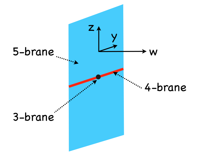
Motivated by these considerations, in this Letter we explore Cascading Gravity with $N=3$, consisting of a 3-brane living on a 4-brane, itself embedded in a 5-brane, together in a 6+1-dimensional bulk, as sketched in Fig. 1. Including tension on the 3-brane, we derive a solution for which $i)$ the bulk metric is non-singular everywhere (except, of course, for a delta-function in curvature at the 3-brane location) and asymptotically flat; and $ii)$ the induced 3-brane geometry is exactly flat.

Since the metric depends on 3 spatial coordinates, to proceed analytically we restrict ourselves to the weak-field approximation, corresponding to sufficiently small tension. For consistency, we check that our solution remains perturbative everywhere. We are currently working on numerically extending these solutions to the non-linear regime of large tension.

Unlike the case of a pure codimension-3 DGP brane in 6+1 dimensions, where the static bulk geometry has a naked singularity for arbitrarily small tension [4], here the bulk metric is completely smooth. This traces back to the cascading mechanism of regulating the propagator: the presence of parent branes removes the power-law divergence in the $4d$ propagator.

As illustrated in Fig. 1, the 3 extra spatial dimensions are denoted by $y,z$ and $w$, with the codimension-1 brane located at $w=0$, the codimension-2 brane at $z=w=0$, and the codimension-3 brane at $y=z=w=0$. Indices in $7d$ are denoted by $A,B,\ldots$, indices in $6d$ by $a,b,\ldots$, in $5d$ by $\alpha,\beta,\ldots$, and finally in $4d$ by $\mu,\nu,\ldots$

In the absence of the $5d$ and $4d$ kinetic terms, the propagator on the codimension-1 brane is of the DGP form [5]

$$G_{6}^{(0)}(z-z^{\prime})=\frac{1}{M_{6}^{4}}\int\frac{{\rm d}\omega}{2\pi}\frac{e^{i\omega(z-z^{\prime})}}{\omega^{2}+q^{2}+m_{7}\sqrt{q^{2}+\omega^{2}}}\,,$$

(3)

where $q^{\alpha}$ is the $5d$ momentum, and $\omega$ is the momentum associated with the $z$ coordinate. The exact $6d$ propagator is then obtained by treating the $5d$ kinetic term as a perturbation localized at $z=0$:

		$\displaystyle G_{6}(z,z^{\prime})=G_{6}^{(0)}(z-z^{\prime})-M_{5}^{3}G_{6}^{(0)}(z)q^{2}G_{6}^{(0)}(-z^{\prime})$		(4)
		$\displaystyle~~~~~~~~~+M_{5}^{6}G_{6}^{(0)}(z)q^{4}G_{6}^{0)}(0)G_{6}^{(0)}(-z^{\prime})+\dots$		(5)
		$\displaystyle=G_{6}^{(0)}(z-z^{\prime})-\frac{G_{6}^{(0)}(z)M_{5}^{3}q^{2}G_{6}^{(0)}(-z^{\prime})}{1+M_{5}^{3}q^{2}G_{6}^{(0)}(0)}\,.$		(6)

In particular the induced propagator on the codimension-2 brane is determined in terms of the integral of the higher dimensional Green’s function:

$$G_{5}^{(0)}(q^{2})=G_{6}(0,0)=\frac{1}{M_{5}^{3}}\frac{1}{q^{2}+g(q^{2})}\,;$$

(7)

$$g(q^{2})\equiv\frac{1}{M_{5}^{3}G^{(0)}_{6}(0)}=\frac{\pi m_{6}}{2}\frac{\sqrt{m_{7}^{2}-q^{2}}}{\tanh^{-1}\,\left(\sqrt{\frac{m_{7}-|q|}{m_{7}+|q|}}\right)}\,.$$

(8)

(For $|q|>m_{7}$ we assume analytic continuation from hyperbolic tangent to its trigonometric counterpart.)

Remarkably, the codimension-1 kinetic term makes the $5d$ propagator finite, thereby regulating the logarithmic divergence characteristic of pure codimension-2 branes. Indeed, $G_{5}^{(0)}\rightarrow M_{7}^{-5}\log(m_{7}q)$ as $M_{6}\rightarrow 0$, and thus $M_{6}$ plays the role of a physical cut-off. As another check, note that in the limit $m_{7}\rightarrow 0$ in which the bulk decouples, we recover the usual DGP result: $G_{5}^{(0)}\sim 1/(q^{2}+m_{6}q)$.

It is straightforward to repeat the same steps to derive the induced $4d$ propagator on the codimension-3 brane.

In the weak-field approximation, the $7d$ line element can be written as ${\rm d}s^{2}=(\eta_{AB}+h_{AB}){\rm d}x^{A}{\rm d}x^{B}$. As shown in Appendix I, there is enough symmetry and gauge freedom to simplify the metric to the form

	$\displaystyle{\rm d}s^{2}$	$\displaystyle=$	$\displaystyle\left(1+\Phi(y,z,w)\right)\left({\rm d}w^{2}+{\rm d}z^{2}+{\rm d}y^{2}\right)$		(10)
		$\displaystyle-$	$\displaystyle\frac{\Theta(w)}{2m_{7}}\partial_{\alpha}\Phi_{0}(y,z){\rm d}x^{\alpha}{\rm d}w$
		$\displaystyle+$	$\displaystyle\left(1-\frac{\Phi(y,z,w)}{4}\right)\eta_{\mu\nu}{\rm d}x^{\mu}{\rm d}x^{\nu}\,,$

where $\Phi_{0}(y,z)\equiv\Phi(y,z,w=0)$ is the induced profile on the codimension-1 brane. Here $\Theta(w)$ is the theta function: $\Theta(w)=+1$ for $w>0$, and $-1$ for $w<0$.

Substituting this ansatz into Einstein’s equations (9), we find that $\Phi$ satisfies

$\displaystyle\left(\Box_{7}+\frac{\delta(w)}{m_{7}}\Box_{6}-\frac{3}{5}\frac{\delta^{2}(z,w)}{m_{7}m_{6}}\Box_{5}\right)\Phi=\frac{8}{5}\frac{\delta^{3}(y,z,w)}{M_{7}^{5}}\Lambda\,.\ \$

(11)

This equation is of the cascading form [12], as reviewed above. The asymptotically flat bulk solution is given by

$$\Phi(y,z,w)=e^{-|w|\sqrt{-\Box_{6}}}\Phi_{0}(y,z)\,,$$

(12)

where the induced profile $\Phi_{0}(y,z)$ satisfies

$$\left(\Box_{6}-m_{7}\sqrt{-\Box_{6}}-\frac{3}{5}\frac{\delta(z)}{m_{6}}\Box_{5}\right)\Phi_{0}=\frac{8}{5}\frac{\delta^{2}(y,z)}{M_{6}^{4}}\Lambda\,.$$

(13)

To solve (13), we Fourier transform to momentum space and use the $6d$ and $5d$ Green’s functions given respectively by (3) and (7). The result is

$$\Phi_{0}(y,z)=\int\frac{{\rm d}q_{y}{\rm d}\omega}{(2\pi)^{2}}\frac{e^{i\omega z}e^{iq_{y}y}g(q_{y})\phi(q_{y})}{\omega^{2}+q_{y}^{2}+m_{7}\sqrt{\omega^{2}+q_{y}^{2}}}\,,$$

(14)

where the Fourier transform of the codimension-2 profile, $\phi(q_{y})=\int{\rm d}ye^{-iq_{y}y}\Phi_{0}(z=0,y)$, satisfies

$$\left(\frac{3}{5}q_{y}^{2}-g\left(q_{y}^{2}\right)\right)\phi(q_{y})=\frac{8}{5M_{5}^{3}}\Lambda\,.$$

(15)

The solution to (15) can be expressed as the sum of a principal part $\mathcal{P}$ and two homogeneous modes:

$$\phi(q_{y})=\frac{8\Lambda}{5M_{5}^{3}}\,\mathcal{P}\left[\frac{1}{\frac{3}{5}q_{y}^{2}-g\left(q_{y}^{2}\right)}\right]+\sum_{\sigma=\pm}C_{\sigma}\delta(q_{y}-\sigma q_{0})\,,$$

where $\frac{3}{5}q_{0}^{2}=g(q_{0}^{2})$. Requiring the field $\Phi_{0}$ to be real imposes $C_{+}=C_{-}\equiv C$, while requiring $\Phi_{0}$ to fall as $y\to 0$ sets $C=0$. Using the resulting expression for $\phi(q_{y})$ into (14) and then into (12), we obtain the final expression for the scalar potential $\Phi(y,z,w)=\frac{8\Lambda}{5M_{6}^{4}}\hat{\Phi}(y,z,w)$:

$\displaystyle\hat{\Phi}\hskip-2.0pt=\hskip-4.0pt\int\frac{{\rm d}\omega{\rm d}q_{y}}{(2\pi)^{2}}\frac{e^{-|w|\sqrt{\omega^{2}+q_{y}^{2}}}e^{i\omega z}e^{iq_{y}y}}{\omega^{2}+q_{y}^{2}+m_{7}\sqrt{\omega^{2}+q_{y}^{2}}}\mathcal{P}\hskip-3.0pt\left[\frac{g(q_{y})}{\frac{3}{5}q_{y}^{2}-g(q_{y})}\right]\,$

(16)

This is our main result. Thanks to the cascading mechanism, which has regularized all potential divergences, this solution is finite everywhere. Figure 2 shows that $\hat{\Phi}(y,z,w)$ is smooth everywhere and decreases with $w$.

As it stands, however, our framework has a ghost [8, 9], as indicated by the poles at $q_{y}=\pm q_{0}$. There are two ways to resolve this issue. One can introduce sufficiently large tension on both the codimension-2 and -3 branes [11]: to remove the ghost, the codimension-2 tension should be $\;\mathrel{\mathstrut\smash{\vtop{\halign{#\cr\raise 2.5pt\hbox{$>$}\cr\lower 2.5pt\hbox{$\sim$}\crcr}}}}\;M_{5}^{3}m_{7}^{2}$, whereas the corresponding bound on the codimension-3 tension is yet to be determined.

Alternatively, one can regularize codimension-2 and -3 branes and include $6d$ Einstein-Hilbert term localized on these objects [9, 12]. Following this route, we demonstrate in Appendix II that the poles do disappear, and that the profile for $\Phi(y,z,w)$ is qualitatively unchanged.

These properties crucially depend on the existence of parent branes with finite Planck masses. Indeed, our solution goes outside the perturbative regime and acquires divergences in the limit $M_{5},M_{6}\rightarrow 0$, consistent with [4].

We are currently extending our solutions to the non-linear regime through numerical analysis. For now, we view the present results as a tantalizing first step towards realizing the idea of Rubakov and Shaposhnikov.

Acknowledgments: We thank G. Dvali and G. Gabadadze for helpful discussions. This work was supported in part by NSERC and Ontario’s MRI.

To proceed further, it is convenient to decompose $h_{ab}$ into its trace and transverse-traceless (TT) parts:

$$h_{ab}=h_{ab}^{6d{\rm TT}}+\frac{\partial_{a}\partial_{b}}{\Box_{6}}h^{c}_{\;c}\,.$$

(18)

From (17), the $6d$TT components satisfy

	$\displaystyle-\frac{M_{7}^{5}}{2}\left(\Box_{7}+\frac{\delta(w)}{m_{7}}\Box_{6}\right)h_{ab}^{6d{\rm TT}}=$
	$\displaystyle\;\;\;\;\;\;\delta(w)\left(T_{ab}^{(6)}-\frac{1}{5}\eta_{ab}T^{(6)}+\frac{1}{5}\frac{\partial_{a}\partial_{b}}{\Box_{6}}T^{(6)}\right)\,.$		(19)

The symmetries of the problem allow a simple expression for the $5d$ components of the $6d$TT part:

$$h_{\alpha\beta}^{6d{\rm TT}}=-\frac{1}{4}\Phi\eta_{\alpha\beta}-\left(\frac{\Box_{5}}{\Box_{6}}-\frac{5}{4}\right)\frac{\partial_{\alpha}\partial_{\beta}}{\Box_{5}}\Phi\,.$$

(20)

This follows from setting $h_{\alpha\beta}^{5d{\rm TT}}=0$, which is consistent with the equations of motion for the case of interest. Substituting into (19), and using $T^{(5)}_{\alpha\beta}=-\delta^{\mu}_{\;\alpha}\delta^{\nu}_{\;\beta}\Lambda\eta_{\mu\nu}\delta(y)$, the resulting equation of motion for $\Phi$ agrees with (11).

We can now be explicit about the form of the various metric components. Combining (18) and (20), we get:

$$h_{\alpha\beta}=-\frac{1}{4}\Phi\eta_{\alpha\beta}-\left(\frac{\Box_{5}}{\Box_{6}}-\frac{5}{4}\right)\frac{\partial_{\alpha}\partial_{\beta}}{\Box_{5}}\Phi+\frac{\partial_{\alpha}\partial_{\beta}}{\Box_{6}}h^{c}_{\;c}\,.\$$

(21)

And since everything is independent of $x^{\mu}$, we get $h_{y\mu}=0$ and $h_{\mu\nu}=-\frac{1}{4}\Phi\eta_{\mu\nu}$. Similarly, from (18) we obtain

	$\displaystyle h_{yz}$	$\displaystyle=$	$\displaystyle\frac{\partial_{y}\partial_{z}}{\Box_{6}}\left(h^{c}_{\;c}-\Phi\right)\;;\;\;h_{zz}=\frac{\partial^{2}_{z}}{\Box_{6}}\left(h^{c}_{\;c}-\Phi\right)+\Phi\;;$
	$\displaystyle h_{yy}$	$\displaystyle=$	$\displaystyle\frac{\partial^{2}_{y}}{\Box_{6}}\left(h^{c}_{\;c}-\Phi\right)+\Phi\,.$		(22)

The is equivalent to (10) after a small diffeomorphism.

When adding a $6d$ Einstein-Hilbert term on the regularized 4-brane, on the top of the usual $5d$ Einstein-Hilbert term of the form ‘$\Box_{5}h_{\alpha\beta}$’ we must consider excitations of transverse modes along the extra dimensions as well as the higher-dimensional mode $h_{zz}$. In the thin-brane limit, however, the excitations along the extra dimension become very massive, so that any term containing $z$-derivatives can be neglected. Meanwhile, $h_{zz}$ survives in the limit. See [12] for details.

In 7$d$ de Donder gauge, the Einstein equations are the same as in (Flat 3-Brane with Tension in Cascading Gravity). Setting $h_{aw}=0$ and $h_{ww}=h^{c}_{\;c}$, we have

$\displaystyle-\frac{M_{7}^{5}}{2}\left(\hskip-2.0pt\Box_{7}+\frac{\delta(w)}{m_{7}}\Box_{6}\hskip-2.0pt\right)\hskip-2.0pth_{ab}=\delta(w)\hskip-2.0pt\left(\hskip-2.0ptT^{(6)}_{ab}-\frac{1}{5}T^{(6)}\eta_{ab}\hskip-2.0pt\right)$

(23)

with $T^{(6)}_{z\alpha}=0$, $T^{(6)}_{zz}=M_{5}^{3}\delta(z)R_{5}/2$, and

	$\displaystyle\hskip-10.0ptT^{(6)}_{\alpha\beta}=-M_{5}^{3}\delta(z)\hskip-3.0pt\left[G_{\alpha\beta}^{(5)}+\frac{1}{2}\left(\Box_{5}h_{zz}\eta_{\alpha\beta}-\partial_{\alpha}\partial_{\beta}h_{zz}\right)\right]\$
	$\displaystyle\hskip 20.0pt-\delta(z)\delta(y)\Lambda\eta_{\mu\nu}\delta^{\mu}_{\alpha}\delta^{\nu}_{\beta}\,.$		(24)

Using this in the $6d$ part of the Einstein equations, we get $h_{zz}=-\psi$, $\Box_{5}h_{yy}=-4\Box_{5}\psi+\partial_{y}^{2}h^{\alpha}_{\,\alpha}$, $h_{\mu y}=0$ and $\Box_{5}h_{\mu\nu}=\Box_{5}\psi\eta_{\mu\nu}+\partial_{\mu}\partial_{\nu}h^{\alpha}_{\,\alpha}$, with

$\displaystyle\left[\Box_{7}+\frac{\delta(w)}{m_{7}}\Box_{6}+\frac{\delta^{(2)}(w,z)}{m_{7}m_{6}}\Box_{5}\right]\psi=\frac{2}{5}\frac{\delta^{(3)}(w,z,y)}{M_{7}^{5}}\Lambda\,.\ \$

(25)

We notice that the kinetic term for $\psi$ is now everywhere positive, signaling that the ghost has been cured. Equation (25) is similar to (11) for $\Phi$, except for a redefinition of $m_{6}$ and $M_{7}$. The profile for $\psi(y,z,w)=-\frac{2\Lambda}{5M_{6}^{4}}\hat{\Psi}(y,z,w)$,

$\displaystyle\hat{\Psi}=\int\frac{{\rm d}\omega{\rm d}q_{y}}{(2\pi)^{2}}\frac{e^{-|w|\sqrt{\omega^{2}+q_{y}^{2}}}e^{i\omega z}e^{iq_{y}y}}{\omega^{2}+q_{y}^{2}+m_{7}\sqrt{\omega^{2}+q_{y}^{2}}}\frac{g(q_{y})}{q_{y}^{2}+g(q_{y})}\,,$

(26)

is similar to that of $\hat{\Phi}$, and, in particular, is free of divergences. The static solution for a codimension-3 brane with tension remains therefore well-defined, at least in the weak field approximation, in a ghost-free set-up.

References

- [1] V. A. Rubakov and M. E. Shaposhnikov, Phys. Lett. B 125, 139 (1983).
- [2] S. Weinberg, Rev. Mod. Phys. 61, 1 (1989).
- [3] Y. Aghababaie, C. P. Burgess, S. L. Parameswaran and F. Quevedo, Nucl. Phys. B 680, 389 (2004) [arXiv:hep-th/0304256].
- [4] G. Dvali, G. Gabadadze and M. Shifman, Phys. Rev. D 67, 044020 (2003) [arXiv:hep-th/0202174].
- [5] G. R. Dvali, G. Gabadadze and M. Porrati, Phys. Lett. B 485, 208 (2000) [arXiv:hep-th/0005016].
- [6] N. Arkani-Hamed, S. Dimopoulos, G. Dvali and G. Gabadadze, arXiv:hep-th/0209227.
- [7] G. R. Dvali, S. Hofmann, and J. Khoury, Phys. Rev. D 76, 084006 (2007) [arXiv:hep-th/0703027].
- [8] S. L. Dubovsky and V. A. Rubakov, Phys. Rev. D 67, 104014 (2003) [arXiv:hep-th/0212222].
- [9] G. Gabadadze and M. Shifman, Phys. Rev. D 69, 124032 (2004) [arXiv:hep-th/0312289].
- [10] R. P. Geroch and J. H. Traschen, Phys. Rev. D 36, 1017 (1987); C. de Rham, JHEP 0801, 060 (2008) [arXiv:0707.0884 [hep-th]].
- [11] C. de Rham, G. Dvali, S. Hofmann, J. Khoury, O. Pujolas, M. Redi and A. J. Tolley, Phys. Rev. Lett. 100, 251603 (2008) [arXiv:0711.2072 [hep-th]].
- [12] C. de Rham, S. Hofmann, J. Khoury and A. J. Tolley, JCAP 0802, 011 (2008) [arXiv:0712.2821 [hep-th]].
- [13] C. de Rham, Can. J. Phys. 87(3): 201–203 (2009) [arXiv:0810.0269 [hep-th]].
- [14] C. de Rham, J. Khoury and A. J. Tolley, to appear.
- [15] G. W. Gibbons, R. Kallosh and A. D. Linde, JHEP 0101, 022 (2001) [arXiv:hep-th/0011225].