Towards an Asymptotic-Safety Scenario for Chiral Yukawa Systems
Abstract
We search for asymptotic safety in a Yukawa system with a chiral UU symmetry, serving as a toy model for the standard-model Higgs sector. Using the functional RG as a nonperturbative tool, the leading-order derivative expansion exhibits admissible non-Gaußian fixed-points for which arise from a conformal threshold behavior induced by self-balanced boson-fermion fluctuations. If present in the full theory, the fixed-point would solve the triviality problem. Moreover, as one fixed point has only one relevant direction even with a reduced hierarchy problem, the Higgs mass as well as the top mass are a prediction of the theory in terms of the Higgs vacuum expectation value. In our toy model, the fixed point is destabilized at higher order due to massless Goldstone and fermion fluctuations, which are particular to our model and have no analogue in the standard model.
I Introduction
The Higgs sector is a crucial building block of the standard model of particle physics and parameterizes the masses of matter fields and weak gauge bosons. This successful parameterization goes along with two problems of the standard model which give rise to the belief that the standard model should be embedded in a larger fundamental framework: the hierarchy problem and the triviality problem. These problems have initiated many further developments.
The triviality problem renders the theory ill-defined from a fundamental point of view, since it inhibits an extension of the standard model to arbitrarily high momentum scales [1, 2, 3, 4, 5, 6]. The scale of the maximum ultra-violet (UV) extension induced by triviality is expected to be related to the Landau pole of perturbation theory. Of course, the Landau pole, i.e., the divergence of a perturbative running coupling at a finite UV scale, in the first place signals the breakdown of perturbation theory. Near the Landau pole, nonperturbative physics can set in and severely modify the picture. So, a study of the triviality problem and the existence of a finite therefore requires a nonperturbative tool. This has also inspired a number of lattice investigations of scalar and chiral Yukawa systems [7, 8, 9, 10].
Whereas the triviality problem is a true conceptual problem of the standard model, the hierarchy problem, i.e., the possible existence of a huge difference between the electroweak scale and an underlying fundamental scale such as the GUT or the Planck scale, is only a problem of unnaturally fine-tuned initial conditions (in this case of the mass parameter in the Higgs potential at the underlying scale).
Solutions to these two problems are often sought by introducing field theories with new degrees of freedom or higher symmetries or by going beyond quantum field theory. The guiding principle of this work is more conservative, as we intend to identify (or rule out) possible solutions within quantum field theory essentially using the same or very similar degrees of freedom of the standard model. Quantum field theory indeed offers a framework for such solutions in terms of Weinberg’s asymptotic safety scenario [11, 12, 13], which has already been investigated in a variety of models ranging from four-fermion models [14, 15, 16], simple Yukawa systems [17], nonlinear sigma models in [18], and extra-dimensional gauge theories [19] to gravity [20, 21]. For the asymptotic-safety scenario to apply, a fixed point of the renormalization group (RG) flow in the space of couplings has to exist. If the system sits on an RG trajectory that hits the fixed point in the UV, the UV cutoff can safely be taken to infinity, and the theory can remain valid to arbitrarily short distance scales.
In fact, a suitable fixed point has recently been identified in a Z2-symmetric Yukawa system [17], serving as a simple toy model for the top-Higgs sector of the standard model. Moreover, a generic mechanism inducing such a fixed point has been proposed which relies on a conformal behavior of the Higgs vacuum expectation value (vev). This conformal-vev mechanism is generated by a dynamical self-balancing of bosonic and fermionic degrees of freedom in the UV. In the simple Z2 model, this balancing actually occurs only for small fractional flavor number . This observation is a strong motivation to consider more realistic Yukawa systems and to explore the potential of the conformal-vev mechanism for the UV problems of the standard model. Another scenario to circumvent the problem of triviality in such a Z2-symmetric Yukawa system in the same framework occurs by coupling the system to a gravitational background [22].
This work is devoted to an investigation of a chiral Yukawa model, serving as a more sophisticated toy-model for the Higgs sector of the standard model (or of a GUT-like theory). The model is designed to have a left-handed chiral sector as is typical for the Higgs sector of the standard model. The number of left-handed fermions is left as a free parameter in order to study the dependence of a potential fixed point on the varying numbers of degrees of freedom. As will be demonstrated by our analysis, this chiral structure facilitates a more boson-dominated Higgs vacuum expectation value which is a prerequisite for conformal-vev mechanism to work. Using the functional RG as a nonperturbative approach, we systematically search for the existence of non-Gaußian interacting fixed points of the RG flow which could allow for an extension of the model to arbitrarily high momentum scales and render the system asymptotically safe.
A particularly attractive by-product of an asymptotically safe Higgs sector is given by the fact that the number of physical parameters is dictated by the number of RG-relevant directions at the fixed point and is thus an inherent property of the model. As this number can actually be smaller than the corresponding one at the Gaußian fixed point (defining the “perturbative” standard model), asymptotic safety can lead to a reduction of physical parameters and hence have more predictive power. For instance, the interacting fixed point in the Z2-invariant toy model has one relevant direction less than the perturbative fixed point. As an immediate consequence, the value of the Higgs mass becomes a prediction once the Higgs vev and the top mass are fixed. For a fixed point of our chiral model discussed in this work, even the top mass can become a prediction, demonstrating the predictive and constraining power of the asymptotic safety scenario.
A crucial question for all nonperturbative techniques is the systematic consistency and reliability of the results. In this work, we compute the RG flow of the model in a systematic derivative expansion of the effective action. This expansion is controlled if the momentum dependence of full effective vertices takes only little influence on the flow. A direct means for measuring this influence is the size of the anomalous dimensions of the fields, since next-to-leading order contributions couple to the leading-order derivative expansion only via terms . Monitoring the size of thus gives us a direct estimate of the reliability of our results. Whereas the anomalous dimensions at the fixed point of the Z2 model were indeed found to be small, the anomalous dimensions at the fixed point of the present model can become large. Hence, the results within the present model have to be taken with a grain of salt. The reason for the difference between the two models lies in the existence of Goldstone bosons as well as massless fermions in the present model which contribute dominantly to the anomalous dimensions. As these massless modes are not present in the standard model, we expect that the leading-order derivative expansion (where ) of the present system can serve as a model for the Higgs-Yukawa sector of a more realistic gauged version. From this viewpoint, the essential idea to have a non-Gaußian fixed point works and provides us with a highly predictive theory.
This paper is organized as follows: in Sect. II, we summarize the essence of the conformal-vev mechanism and introduce the concept of asymptotic safety. Sect. III discusses the nonperturbative construction of the effective action in terms of the functional RG. The fact that the resulting flow equations do not support asymptotic safety in the symmetric regime is briefly elucidated in Sect. IV. In Sect. V, the regime of spontaneous symmetry breaking is explored to leading order, revealing non-Gaußian fixed points with physically appealing properties. The resulting predictive power of the asymptotic-safety scenario is described in Sect. VI. Sect. VII summarizes the problems of the present toy-model occurring at next-to-leading order in the derivative expansion. Conclusions are drawn in Sect. VIII. Technical details on the derivation of the flow equations are given in the appendices.
II An asymptotic-safety scenario for Yukawa Systems
II.1 Conformal vacuum expectation value
The model building of the present work is strongly motivated by qualitative considerations about the loop contributions to the running of the dimensionless version of the bosonic field expectation value in the regime of spontaneous symmetry breaking (SSB) where . Our central idea is that the contributions with opposite sign from bosonic and fermionic fluctuations to the vev can be balanced such that the vev exhibits a conformal behavior, . Here, is the scale at which we consider the couplings of the system. The dimensionless squared vev has a flow equation of the form
| (1) |
If the interaction terms are absent, the Gaußian fixed point is the only conformal point, corresponding to a free massless theory. If the interaction terms are nonzero, e.g., if the couplings approach interacting fixed points by themselves, the sign of these terms decides about a possible conformal behavior. A positive contribution from the interaction terms gives rise to a fixed point at which can control the conformal running over many scales. If they are negative, no physically acceptable conformal vev is possible. Since fermions and bosons contribute with opposite signs to the interaction terms, the existence of a fixed point crucially depends on the relative strength between bosonic and fermionic fluctuations. More specifically, the bosons have to win out over the fermions.

In Fig. 1 (taken from [17]), we sketch various options for the flow of the dimensionless squared vev . The solid line depicts the free massless theory with a trivial Gaußian fixed point at . If the fermions dominate, the interaction terms are negative and the fixed point is shifted to negative values (being irrelevant for physics), cf. dotted line. If the bosonic fluctuations dominate, the flow develops a non-Gaußian fixed point at positive values . This can support a conformal behavior over many orders of magnitude, cf. dashed line. This fixed point is UV attractive, implying that the vev is a relevant operator near the fixed point. If the interaction terms are approximately independent, the slope of near the fixed point is still close to , corresponding to a critical exponent and a persistent hierarchy problem. An improvement of “naturalness” could arise from a suitable dependence of the interaction terms that results in a flattening of the flow near the fixed point, cf. dot-dashed line. Whether or not this happens in a specific model is a prediction of the theory which needs to be deduced from the theory by nonperturbative methods.
In this work, we construct a model with standard-model-like symmetries along this line of research. We introduce left-handed fermion species () and one right-handed fermion , as well as complex bosons . All fields live in the fundamental representation of the left-handed chiral symmetry group U. The Yukawa coupling is then realized by a term . This chiral Yukawa system mimics the coupling between the standard-model Higgs scalar and the left- and right-handed components of the top quark, also involving Yukawa couplings to the left-handed bottom (for ) and further bottom-like quarks (for ) in the same family. If the scalar field develops a vev upon symmetry breaking, the top quark acquires a Dirac mass, whereas the bottom-type quarks remain massless (similar to neutrinos in the standard model). For , we ignore the Yukawa coupling in our model, which provides for a mass term for the bottom quark in the standard model, since it does not generalize to other .

In comparison to left-right symmetric models, this model has an interesting new feature concerning the relative weight of the boson interaction terms contributing to the renormalization of the dimensionless vev (see figure 2): diagrammatically speaking, the inner structure of fermion/boson components in the fermion loop for a specific choice of external boson legs is fully determined. On the other hand, the boson loop obtains contributions from all components and so is linear in . In this way, serves as a control parameter for boson dominance and for the potential existence of a non-Gaußian fixed point. Already at this qualitative level of the discussion, it is worthwhile to stress that the standard model has such a left-right asymmetric structure which can support the conformal-vev fixed point.
II.2 Flow equation and asymptotic safety
In the asymptotic-safety scenario of a quantum field theory, the microscopic action to be quantized is a priori unknown. A construction of a renormalizable theory is possible if a suitable fixed point exists in the space of all possible action functionals, i.e., in theory space. This theory space is spanned by all possible operators which can be constructed from the chosen degrees of freedom and which are compatible with the desired symmetries. If such a fixed point exists the microscopic action to be quantized can be constructed from the properties of the fixed point and thus is a prediction itself.
The framework for a nonperturbative construction of renormalizable field theories is provided by the functional RG which can be formulated in terms of a flow equation for the effective average action , the Wetterich equation [23]:
| (2) |
Here, is the second functional derivative with respect to the field , the latter representing a collective field variable for all bosonic or fermionic degrees of freedom, and denotes a momentum-dependent regulator function that suppresses IR modes below a momentum scale . The solution of the Wetterich equation provides an RG trajectory in theory space, interpolating between the bare action to be quantized and the full quantum effective action , being the generating functional of 1PI correlation functions; for reviews, see [24].
The effective average action can be parameterized by a possibly infinite set of generalized dimensionless couplings . Then, the Wetterich equation provides us with the flow of these couplings . A fixed point is defined by
| (3) |
The fixed point is non-Gaußian, if at least one fixed-point coupling is nonzero . If the RG trajectory flows into a fixed point in the UV, the UV cutoff can safely be taken to infinity and the theory can be considered as fundamental.
In addition to being fundamental, we also want the theory to be predictive. For this, let us consider the fixed-point regime, where the flow can be linearized,
| (4) |
The critical exponents correspond to the negative of the eigenvalues of the stability matrix . They allow for a classification of physical parameters: Whereas all eigendirections with die out towards the IR and thus are irrelevant, all relevant directions with increase towards the IR and thus determine the macroscopic physics (for the marginal directions , it depends on the higher-order terms in the expansion about the fixed point). Hence the number of relevant and marginally-relevant directions determines the number of physical parameters to be fixed. The theory is predictive if this number is finite. In the case of the Gaußian fixed point , the present construction corresponds to the standard perturbative power-counting analysis and the critical exponents are equal to the power counting dimensions of the couplings.
If a critical exponent is much larger than zero, say of , the RG trajectory rapidly leaves the fixed-point regime towards the IR. Therefore, separating a typical UV scale where the system is close to the fixed point from the IR scales where, e.g., physical masses are generated requires a significant fine-tuning of the initial conditions.
For the flow towards the IR, the linearized fixed-point flow Eq. (4) generally is insufficient and the full nonlinear functions have to be taken into account. Even the parameterization of the effective action in terms of the same degrees of freedom in the UV and IR might be inappropriate. Nevertheless, we use the same bosonic and fermionic degrees of freedom on all scales in the present work, since we specifically want to address the question whether standard-model IR degrees of freedom can have an interacting UV completion.
III Renormalization flow of chiral Yukawa systems
III.1 Derivative expansion
In the present work, we investigate a Yukawa theory with chiral fermions including one right-handed fermion and left-handed fermions. The fermions are coupled to complex bosons via a simple Yukawa interaction. We span the theory space by a truncated action functional in a derivative expansion, which reads at next-to-leading order
| (5) | |||||
The fermion fields and have standard kinetic terms but can acquire different wave function renormalizations and . The index runs from to . The projections on the left-/right-handed fermion contributions are carried out via the projection operators
| (6) |
The bosonic sector involves a standard kinetic term with wave function renormalization and an effective potential . Defining the invariant , the effective potential can be expanded in powers of . The bosons can also be expressed in terms of a real field basis by defining
| (7) |
where . The truncated effective action (5) including the Yukawa interaction is invariant under U transformations of the left-handed fermion and the boson as well as U transformations of the right-handed fermion and the boson.
All the parameters in the effective average action are understood to be scale dependent, which is indicated by the index .
The flow of the wave function renormalizations and can be expressed in terms of scale-dependent anomalous dimensions
| (8) |
Setting the anomalous dimensions to zero defines the leading-order derivative expansion. At next-to-leading order, it is important to distinguish between and as they acquire different loop contributions, see below.
In order to fix the standard RG invariance of field rescalings, we define the renormalized fields as
| (9) |
For the fixed-point search, it is useful to introduce dimensionless renormalized quantities
| (10) | |||||
| (11) | |||||
| (12) |
Detailed information about the derivation of the flow equations for this truncation in arbitrary spacetime dimensions is given in App. B. For our purposes, we use a linear regulator function which is optimized for the present truncation [25]. The flow of the effective potential in terms of threshold functions which are given in App. A reads
| (13) | |||||
where the primes denote derivatives with respect to , and . For the symmetric phase (SYM), we expand the effective potential around zero field,
| (14) |
For the SSB phase, where the minimum of the effective potential acquires a nonzero value , we use the expansion
| (15) | |||||
Given the flow of (13), the flows of or in both phases can be read off from an expansion of the flow equation and a comparison of coefficients. For the flow of , we use the fact that the first derivative of vanishes at the minimum, . This implies
| (16) |
The explicit flow equations for the running parameters will be given in the following sections for the SYM and the SSB phase separately. Note that the expansion coefficients in Eqs. (14) and (15) are not identical. Since there is little risk that the notation of the different regimes interferes with each other, we refrain from introducing different symbols.
In the SSB regime, the flow of the Yukawa coupling and the scalar anomalous dimension for the Goldstone mode can, in principle, be different from that of the radial mode. As the Goldstone modes as such are not present in the standard model, we compute the Yukawa coupling and the scalar anomalous dimension by projecting the flow onto the radial scalar operators in the SSB regime. Note that this strategy is different from that used for critical phenomena in other Yukawa or bosonic systems, where the Goldstone modes can dominate criticality.
Accordingly, the flow of the Yukawa coupling can be derived (see App. C), and we end up with
| (17) | |||||
Finally, we list the expressions for the anomalous dimensions
| (18) | |||||
| (19) | |||||
| (20) |
The arguments of the threshold functions have to be evaluated at the minimum of the effective potential. In the following sections, we will concentrate on the case of dimensions.
Let us emphasize that the derivative expansion has already been tested in various Yukawa systems and has proved to yield qualitatively and quantitatively accurate results. RG flows for Yukawa systems have been successfully studied in QCD [26], critical phenomena [27], quantum phase transitions [28] and ultra-cold fermionic atom gases [29].
III.2 Parameter constraints
Let us finally discuss several constraints on the couplings as, e.g., dictated by physical requirements as well as by our truncation. As our truncation is based on a derivative expansion, satisfactory convergence is expected if the higher derivative operators take little influence on the flow of the leading-order terms. In the present case, the leading-order effective potential receives higher-order contributions only through the anomalous dimensions. Therefore, convergence of the derivative expansion requires
| (21) |
This condition will serve as an important quality criterion for our truncation. The SYM regime is characterized by a minimum of at vanishing field. A simple consequence is that the mass term needs to be positive. Also, the potential should be bounded from below, which in the polynomial expansion translates into a positive highest nonvanishing coefficient,
| (22) |
In the SSB regime, the minimum must be positive, , the potential should be bounded, and in addition the potential at the minimum must have positive curvature,
| (23) |
Finally, Osterwalder-Schrader positivity requires
| (24) |
Beyond that, there are no constraints on the size of the couplings as in perturbation theory.
IV The Symmetric Regime (SYM)
Let us first investigate the fixed-point structure of the system in the symmetric regime. We restrict ourselves to four dimensions and expand the effective action using the ansatz (14). Now and in the following we will suppress the index at the parameters of the truncation for notational convenience. The flow equations are evaluated at the minimum of the effective potential, which is at in the symmetric regime, and we replace , , . In this case, the next-to-leading order flow equations up to second order in the effective potential read
| (25) | |||||
| (26) | |||||
We observe that the flow equation of a coupling involves . For the Yukawa coupling we obtain
| (27) |
In particular, all contributions from typical vertex triangle diagrams vanish in the SYM regime. At leading order in a derivative expansion where , the Yukawa coupling does not flow in the SYM regime. At next-to-leading order, we also have to take into account the anomalous dimensions
| (28) | |||||
| (29) | |||||
| (30) |
For an interacting fixed point with a non-vanishing to exist, the prefactor in the flow equation for the Yukawa coupling would have to vanish at some point in parameter space. This implies that the different anomalous dimensions need to have a relative minus sign. From Eq. (28), we read off that a relative sign change requires either or . Both options would clearly be in conflict with the validity bounds of the derivative expansion, demanding at least for .
Therefore, a nontrivial fixed point of the Yukawa coupling in the SYM regime based on the criterion – even if it existed – would be beyond the reliability bounds of the derivative expansion. Within the validity regime of our truncation, we thus find only the Gaußian fixed point for the Yukawa coupling . Since the flow of the Yukawa coupling is proportional to itself, an initial zero value for will leave the system non-interacting at for all scales. The remaining interacting system is purely bosonic and does not show any nontrivial fixed point in agreement with triviality of theory. We conclude that the chiral Yukawa model in the SYM regime is not asymptotically safe within the part of theory space spanned by our truncation.
V The Regime of Spontaneous Symmetry Breaking (SSB)
Let us continue our fixed-point search in the broken-symmetry regime. The flow equations have a richer structure here, since the coupling to the condensate can mediate further effective interactions. Most importantly, the broken regime can support the fixed-point scenario with a conformal vev.
V.1 Fixed-point search to leading order
For the fixed-point search, we use a polynomial expansion of the effective potential about its minimum, cf. Eq. (15). As a check of the quality of this expansion, the convergence properties of physical quantities have to be determined with respect to increasing orders in this expansion. In general, we expect that this expansion gives a good approximation of the full effective potential only in the vicinity of the potential minimum. Nevertheless, this can still lead to sufficient information for a quantitative estimate of a variety of physical quantities, as they are mostly related to properties of the potential near the minimum.
For a first glance, we use the simplest nontrivial approximation of the effective potential, , which facilitates a purely analytical treatment of the fixed-point equations. The flow of the effective potential (13), evaluated around the minimum, then boils down to flows for and , with all other couplings being zero, i.e., , and for . We also confine ourselves to the leading-order approximation in the derivative expansion, where the anomalous dimensions vanish, . The flow equations in this approximation read explicitely
| (31) | |||||
| (32) |
and for the Yukawa coupling
| (33) | |||||


The resulting set of fixed-point equations can be solved analytically. For a given , we obtain a large number of fixed points but only up to two fixed points fulfill the physical constraints given in section III.1. For , we find only one admissible non-Gaußian fixed point (NGFP). For , two admissible NGFPs occur. For , there is again only one NGFP, whereas larger do not give rise to any physically admissible fixed points. The fixed-point values , , and as a function of can be read off from figure 3.
The universal critical exponents can be deduced from the linearized flow around this fixed point, cf. Eq. (4),
| (34) |
where in the present simple truncation. The expansion coefficients form the stability matrix, the eigenvalues of which correspond to the critical exponents apart from a minus sign. The critical exponents as a function of are shown in Fig. 4 for this simple truncation. It is remarkable that one NGFP has two relevant directions and the other even only one relevant direction with a positive critical exponent. This implies that the corresponding model is fixed by only two or one physical parameter, respectively. This should be compared to the Gaußian fixed point with perturbative critical exponents of the order , , and , implying that 3 physical parameters need to be fixed for Gaußian models. Moreover, both NGFPs exhibit a largest critical exponent being smaller than the perturbative maximal value, . As a consequence, these models defined at the NGFPs have an improved hierarchy behavior.
V.2 Benchmark fixed point for
For further investigations and by way of example, we concentrate on one particular fixed point. We use a fixed point with only one relevant direction, as it is phenomenologically most appealing due to the reduction of physical parameters. We choose in the following, since the corresponding fixed point does not give rise to extreme coupling values, implying numerical stability. In addition, this particular value of may also be of relevance for certain unification scenarios.
Furthermore, we extend the lowest-order polynomial expansion studied above to higher operators, cf. Eq. (15),
| (35) |
where labels the higher orders. From a technical viewpoint, the fixed-point analysis becomes much more involved at higher orders. In particular, we have not found any analytical solutions to the higher-order fixed-point equations. Due to the intrinsic nonlinearity of the fixed-point equations, also a numerical search is nontrivial: a complete identification of all possible fixed points appears out of reach.
Therefore, we start with the assumption that the simple truncation involving only and gives already a satisfactory fixed-point estimate. As a next step, we can search for a fixed-point of the subsequent higher-order system in the vicinity of the previous lower-order fixed point. This procedure turns out to be self-consistent and can be iterated to higher orders. The results for the associated fixed-point values up to are summarized in Tab. 1.
| 55.8 | 0.0174 | 12.11 | - | - | - | - | |
| 56.0 | 0.0158 | 12.09 | -115 | - | - | ||
| 57.4 | 0.0152 | 12.13 | -152 |
The resulting fixed-point values show a satisfactory convergence behavior, indicating that the polynomial expansion is quantitatively reliable already at low orders. This convergence property is also confirmed by the form of the fixed-point potential in a finite environment of the expansion point , as is depicted in Fig. 5: The fixed-point potential of Mexican-hat type remains quantitatively stable under the inclusion of higher orders – even away from the minimum .
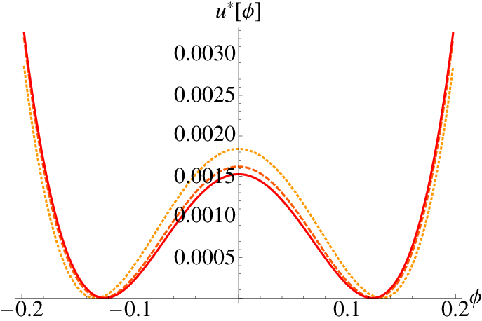
Whereas the fixed-point potential is scheme dependent, also the stability of the universal critical exponents can be checked under the inclusion of higher orders in the polynomial expansion. The results for the associated critical exponents up to are summarized in Tab. 2. The leading exponents vary only on the 10%-level upon the inclusion of higher-order terms. Most importantly, the number of relevant directions is not changed at higher orders, and the maximal critical exponent tends to smaller values at higher orders which leads to an improved hierarchy behavior. We conclude that the fixed point exists at leading-order in the derivative expansion. It possesses many desirable properties and can well be approximated by a polynomial expansion.
| 1.294 | -0.143 | -3.94 | - | - | - | - | |
| 1.167 | -0.170 | -2.50 | -5.53 | -13.61 | - | - | |
| 1.056 | -0.175 | -2.35 | -4.97 | -8.49 | -14.02 | -25.54 |
VI Predictive power of asymptotically-safe Yukawa systems
We illustrate the predictive power of an asymptotically safe Higgs sector, using the flow of our system in the local-potential approximation as a model in its own right.
Perturbatively, our model would be defined by three bare parameters if the microscopic theory is initiated near the Gaußian fixed point. These three parameters can be specified, e.g., in terms of the bare Yukawa coupling , the coupling , and the scalar mass term in units of the UV cutoff . 11 1 Owing to triviality at the Gaußian fixed point, the cutoff cannot be removed. Strictly speaking, this leads to a lack of universality, such that the couplings of higher-dimensional operators also correspond to physical parameters. Their influence on the IR physics is, however, suppressed by corresponding inverse powers of the UV cutoff .
The bare parameters can be fixed in terms of renormalization conditions. The latter ultimately relates these parameters to the physical IR parameters: the Higgs vev , the Higgs mass and the top mass . These, in turn, are related to the renormalized couplings by
| (36) |
(The bottom-type quarks remain massless in our model.)


This counting of independent physical parameters changes drastically if the system originates from the non-Gaußian fixed point in the limit of an infinite UV cutoff. As the non-Gaußian fixed point has only one relevant direction, there is only one physical parameter which we relate to the vev GeV. In fact, fixing to its physical value merely corresponds to fixing the absolute scale. Dimensionless couplings or mass ratios are even independent of this fixing scale and thus are completely parameter-free predictions of the theory.
In practice, we have to start the flow at some finite value of the auxiliary UV cutoff (in arbitrary units), solve the flow, and then associate the resulting value of with its correct value in physical units. This also fixes the value of in units of, say, GeV. In the model with , we then end up with a top and a Higgs mass at the IR scale
| (37) |
where the proportionality factors are approached in the limit . In this limit, this result is robust as we vary the UV cutoff, which demonstrates the cutoff independence of our prediction. As a result, the top and the Higgs mass are pure predictions of the theory itself.
Whereas the Higgs mass is of the order of the vev as expected, GeV for GeV, the top mass is significantly larger in our model: GeV. This is an indirect consequence of the comparatively large value of the fixed point of the Yukawa coupling. In order to elucidate this relation, let us note that the flow can be subdivided into three different regimes: first, the UV fixed-point regime where all couplings stay close to their fixed point values; second, a crossover region where all couplings run fast; and third, a freeze-out region in the IR where the dimensionful vev builds up and induces decoupling and a subsequent approach to the generically frozen IR values.
The dynamics in the crossover region is an intrinsic parameter-free property of the model that occurs only in a rather narrow window of momentum scales. Hence, the couplings have only a finite “RG time” – similar to the number of -foldings in inflationary cosmology – to run from their UV initial conditions to their IR-frozen values. As the initial fixed-point Yukawa coupling in our model is large, a sizeable IR value remains and gives rise to a large top mass. The same mechanism has been identified in the Z2-symmetric Yukawa system in [17] even for the case with two relevant directions. There, the top mass is, in principle, a physical parameter to be fixed; still, the finite number of crossover -foldings leads to a lower bound on the Higgs mass.
Realistic scenarios with a physical value of the top mass require either a smaller fixed-point Yukawa coupling, or a sufficiently large number of crossover -foldings that facilitates a long running of the Yukawa coupling to its physical value. As the number of -foldings of the crossover window is mainly dictated by the RG speed at which the physical vev builds up, large numbers of -foldings can occur if the largest critical exponent dominating the flow is small. We conclude that a reduced hierarchy problem and a realistic value of the top mass can go hand in hand with each other.
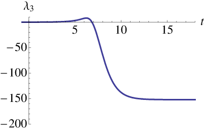
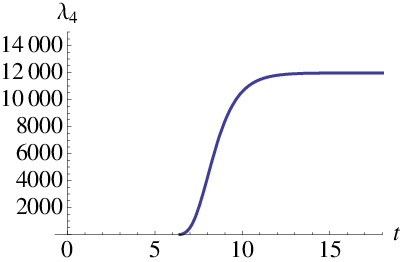
Finally, we have to address an artifact of our flow in the IR. As can be read off from Fig. 6, the perturbatively marginal couplings and still exhibit a slow log-like running in the IR. In our present set of flow equations, the source of this running can be traced back to the Goldstone modes which are a particularity of our model, but are not present in the standard model. However, even if we considered the Goldstone modes as physical, the log-like running is still an artifact of our truncation in the IR. This artifact arises from the Cartesian decomposition of the scalar field, (we suppress flavor indices in the following argument) where the vev is associated with the direction and is populated with Goldstone modes. This decomposition leads to log-like divergencies in the diagrams with internal loops coupling to external legs. However, as becomes clear from a proper nonlinear decomposition of the scalar field , the true Goldstone modes encoded in the field do not couple to the radial mode via the potential, as is independent of . We conclude that the log-like running would be absent in a proper nonlinear field basis in the broken regime [30].
In practice, we read off our estimates for the IR values of and at a dynamically defined scale . For the identification of this scale, we note that higher-order couplings are not affected by the Cartesian basis and safely flow to zero due to the leading-order Gaußian flow,
| (38) |
as expected, see Fig. 7. We define the scale by that scale at which the coupling approaches its zero IR fixed point from above within an accuracy of . The IR predictions listed in Eq. (37) have been read off at this scale. Of course, in the presence of this flow artifact, these predictions actually depend on the choice of . Nevertheless, the generic mechanisms in the UV and crossover regimes outlined above are not affected by the IR artifact.
VII Properties of the derivative expansion at next-to-leading order
In the preceeding section, we have analyzed the chiral Yukawa model in a derivative expansion of the effective action. As a simple criterion for this expansion to be valid, the anomalous dimensions measuring the influence of higher-derivative terms should be small, cf. Eq. (21).
As a first check of this criterion, we use our fixed-point results from the lowest-order polynomial expansion in the local-potential approximation and insert them into the right-hand sides of the anomalous dimensions Eqs. (18)-(20). For this estimate, we ignore the RG improvement in the form of the back-reactions of nonzero ’s on the flow of the couplings. The results as a function of are shown in Fig. 8. Whereas the criterion (21) is satisfied for and for , the anomalous dimension of the right-handed fermion violates the criterion for all . The violation is dramatic for the fixed point with two relevant directions and still substantial for the fixed point with one relevant direction.
One reason for the size of lies in the fact that the massless Goldstone modes and massless bottom-type fermions contribute strongly. This is because they (i) are not damped by massive threshold effects induced by couplings to the condensate, and (ii) contribute with a large multiplicity . We conclude that the leading-order derivative expansion does not provide for self-consistent estimates of the fixed-point structure of the chiral Yukawa model as such. Nevertheless, since the Goldstone as well as the massless fermion modes are not present in the standard model but a particularity of our reduced toy model, we expect that the local-potential approximation of the present model provides for a better picture of a possible fixed-point structure of the standard-model Higgs sector than the literal version of our model including its massless modes.
It is still an interesting question within the chiral Yukawa model, whether the nonlinearities induced by the anomalous dimension gives rise to admissible fixed points if the full RG improvement is taken into account. For this, we have first followed the evolution of our leading-order fixed points upon gradually switching on the anomalous dimensions. Our numerical results are compatible with a destabilization of this fixed point, potentially going along with an annihilation with other fixed points. A numerical search of further admissible fixed points upon the full inclusion of the anomalous dimension remained inconclusive. Owing to the high degree of nonlinearity of the coupled equations, a systematic search in this high-dimensional parameter space is computationally expensive and beyond the scope of the present work.


VIII Conclusions
We have explored a new possible route to asymptotically safe Yukawa systems with a chiral UU symmetry, similar to the Higgs-top sector of the standard model. This work is motivated by the fact that an asymptotically safe Yukawa sector can solve the triviality problem of the standard-model Higgs sector and potentially improve on the hierarchy problem, both of which represent genuine problems related to the UV stability and completion of standard-model particle physics. In our scenario proposed in [17], asymptotic safety is based on a conformal Higgs expectation value that induces a non-Gaußian UV fixed point for all essential couplings.
This conformal behavior can arise from the dynamics of the theory as a consequence of a balancing between fermionic and bosonic fluctuation contributions to the running of the vev. More specifically, since bosonic fluctuations need to dominate, the existence of this conformal-vev behavior depends on the algebraic structure of the theory. It is a central result of our work that chiral models with an asymmetry between left- and right-handed fermions in fact support this boson dominance.
Our quantitative investigations are based on the functional RG, using the derivative expansion as a nonperturbative approximation scheme for a systematic calculation of the quantum effective action. To leading-order (local-potential approximation), our left-right asymmetric model exhibits the desired non-Gaußian fixed points for . Whereas a physically admissible non-Gaußian fixed point establishes the existence of the Yukawa model as a fundamental UV complete quantum field theory, the physical properties of such a UV completion are quantified by the non-negative critical exponents of this fixed point. Their number corresponds to the number of physical parameters, and their value is a measure of the naturalness of a large hierarchy (between, say, the Planck and the electroweak scale).
Most importantly, one of the admissible fixed points has only one positive critical exponent. This implies that only one physical parameter has to be fixed, e.g., the vev GeV, whereas all other IR quantities such as the Higgs or the top mass are a pure prediction of the theory. Moreover, this critical exponent is also smaller than the corresponding value in the perturbative domain, such that the hierarchy behavior is substantially improved.
Unfortunately, the fixed point in our toy model is destabilized at higher order in the derivative expansion due to massless Goldstone and fermion fluctuations. As the latter are a particularity of our model and are not present in the standard model, we expect the results from the local-potential approximation to be of high relevance for a more realistic model of the standard-model Higgs sector. On the other hand, our results have proved robust under an extension of the approximation scheme in the boson effective potential.
As a main result of the present study, a number of conclusions about the requirements for a more realistic model can be drawn. (1.) The appearance of the conformal-vev mechanism depends crucially on the algebraic structure of the theory. Boson dominance is required and can be induced by a chiral left-right asymmetry. (2.) If the conformal vev breaks a continuous global symmetry, Goldstone bosons are generated. As they are not controlled by threshold effects, they may have the tendency to destabilize the UV fixed point. A model with spontaneous breaking of gauged symmetries will not be affected by this problem. (3.) Even though the threshold effects of the conformal vev are nonperturbative, our mechanism does technically not require strong coupling. Comparatively small UV fixed-point couplings would also be allowed if not phenomenologically preferred. (4.) The present model predicts a very large top mass. For a realistic top mass, either the Yukawa UV fixed-point value should not be too large or the crossover from the UV regime to the IR freeze-out should extend over many “-foldings”, i.e., a larger range of RG time.
These requirements together with the remarkable predictive power of our scenario are a strong motivation to extend the present set of ideas to gauged chiral Yukawa models, thereby making another step towards a realistic standard-model Higgs sector.
Acknowledgements.
The authors are grateful to J. M. Pawlowski for interesting discussions and helpful comments. This work was supported by the DFG under contract No. Gi 328/5-1 (Heisenberg program) and FOR 723.Appendix A Threshold functions
The boson cutoff we use is given by:
| (39) |
where , and the fermion regulator is chosen such that . Using this regulator in the Wetterich equation, we can perform all momentum integrations analytically. The result can be given in terms of threshold functions which read
| (40) | |||||
where we have defined .
Appendix B Derivation of the effective potential flow
For the flow of the effective potential, we project the Wetterich equation onto constant bosonic fields and vanishing fermionic fields,
| (41) |
where is the spacetime volume. We have to evaluate the r.h.s of Eq. (41), for which we need the matrix. Taking care of the partly Grassmann-valued field components and the Fourier conventions, is derived by
with
The transposition refers to flavor as well as Dirac indices. For a proper IR regularization, a regulator which is diagonal in field space is sufficient and convenient,
with a matrix for the bosonic sector
cf. App. A and an matrix for the fermionic sector
The matrix has the same block form as the regulator. Therefore, we can evaluate the bosonic and fermionic parts separately. We start with the bosonic part. Inverting the matrix, multiplying with the derivative of the regulator, and taking the supertrace yields
where . Introducing and as the dimension of the representation of the Dirac algebra, the fermionic contribution reads
Adding both parts and using the optimized regulator introduced in App. A, we get
where the threshold functions are defined in Eqs.(40). In terms of dimensionless quantities defined in Eq. (10), the potential flow turns into Eq. (13) in the main text.
Appendix C Derivation of the Yukawa coupling flow
For the derivation of the flow of the Yukawa coupling, we first separate the bosonic field into a vacuum expectation value (vev) and a purely radial deviation from the vev, since we are mainly interested in the Yukawa coupling between the fermions and the radial mode.
setting all Goldstone components to zero. The projection of the Wetterich equation onto the flow of the Yukawa coupling reads
| (42) |
The vertical line indicates that the equation is evaluated at . Next, we can decompose the matrix into two parts. One part, which we call , contains only and is independent of the fluctuations. The remaining part, , contains all fluctuating fields. Inserting this into equation (42) and expanding the logarithm
| (43) | |||||
only the term to third power in survives the projection onto . Performing the matrix calculations and taking the supertrace, we get
where the potential on the right hand side is evaluated at the minimum . Using the optimized regulator and the threshold functions as defined in App. A and switching over to dimensionless quantities, we end up with the representation (17) given in the main text.
Appendix D Derivation of the anomalous dimensions
For the derivation of the flow of , we decompose the bosonic field as in App. C. The projection of the Wetterich equation onto the boson kinetic term leads us to
| (44) | |||||
Again, we have decomposed the matrix into two parts, one part containing the vev and the other part containing all fluctuating fields. As done in App. C, we have expanded the logarithm as in Eq. (43), but this time only the second order contributes. Calculating the r.h.s of Eq. (44), results in
where the potential is evaluated at the minimum. Using the optimized regulator together with the threshold functions as defined in App. A and again introducing dimensionless quantities, we end up with
where we have used , and the right hand side has to be evaluated on the vev.
For the fermionic anomalous dimensions, the procedure is the same. We start with
| (45) |
and get
and
respectively. Using the optimized regulator the result read in terms of dimensionless quantities
| (46) |
and
| (47) |
References
- [1] K. G. Wilson and J. B. Kogut, Phys. Rept. 12, 75 (1974).
- [2] M. Luscher and P. Weisz, Nucl. Phys. B 295, 65 (1988); Nucl. Phys. B 318, 705 (1989).
- [3] A. Hasenfratz, K. Jansen, C. B. Lang, T. Neuhaus and H. Yoneyama, Phys. Lett. B 199, 531 (1987).
- [4] U. M. Heller, H. Neuberger and P. M. Vranas, Nucl. Phys. B 399, 271 (1993) [arXiv:hep-lat/9207024].
- [5] D. J. E. Callaway, Phys. Rept. 167, 241 (1988).
- [6] O. J. Rosten, arXiv:0808.0082 [hep-th].
- [7] J. Smit, Nucl. Phys. Proc. Suppl. 17, 3 (1990); J. Shigemitsu, Nucl. Phys. Proc. Suppl. 20, 515 (1991); K. Jansen, Phys. Rept. 273, 1 (1996) [arXiv:hep-lat/9410018].
- [8] I. H. Lee, J. Shigemitsu and R. E. Shrock, Nucl. Phys. B 334, 265 (1990); Nucl. Phys. B 330, 225 (1990); R. E. Shrock, “Lattice Yukawa Models”, in M. Creutz, ed. Quantum Fields on the Computer, pp. 150 - 210 (World Scientific, Singapore, 1992).
- [9] J. Kuti, L. Lin and Y. Shen, Phys. Rev. Lett. 61, 678 (1988); Z. Fodor, K. Holland, J. Kuti, D. Nogradi and C. Schroeder, PoS LAT2007, 056 (2007) [arXiv:0710.3151 [hep-lat]]. P. Gerhold, K. Jansen and J. Kallarackal, arXiv:0810.4447 [hep-lat]; P. Gerhold and K. Jansen, JHEP 0710, 001 (2007) [arXiv:0707.3849 [hep-lat]]; JHEP 0709, 041 (2007) [arXiv:0705.2539 [hep-lat]].
- [10] K. Jansen, J. Kuti and C. Liu, Phys. Lett. B 309, 119 (1993) [arXiv:hep-lat/9305003]; Phys. Lett. B 309, 127 (1993) [arXiv:hep-lat/9305004].
- [11] S. Weinberg, in C76-07-23.1 HUTP-76/160, Erice Subnucl. Phys., 1, (1976).
- [12] R. Percacci, arXiv:0709.3851 [hep-th].
- [13] S. Weinberg, arXiv:0903.0568 [hep-th]
- [14] B. Rosenstein, B. J. Warr and S. H. Park, Phys. Rev. Lett. 62, 1433 (1989); K. Gawedzki and A. Kupiainen, Phys. Rev. Lett. 55, 363 (1985); C. de Calan, P. A. Faria da Veiga, J. Magnen and R. Seneor, Phys. Rev. Lett. 66, 3233 (1991).
- [15] H. Gies, J. Jaeckel and C. Wetterich, Phys. Rev. D 69, 105008 (2004) [arXiv:hep-ph/0312034].
- [16] J. M. Schwindt and C. Wetterich, arXiv:0812.4223 [hep-th].
- [17] H. Gies and M. M. Scherer, arXiv:0901.2459 [hep-th].
- [18] A. Codello and R. Percacci, arXiv:0810.0715 [hep-th].
- [19] H. Gies, Phys. Rev. D 68, 085015 (2003) [arXiv:hep-th/0305208].
- [20] M. Reuter, Phys. Rev. D 57, 971 (1998) [arXiv:hep-th/9605030]; O. Lauscher and M. Reuter, Phys. Rev. D 65, 025013 (2002) [arXiv:hep-th/0108040]; Class. Quant. Grav. 19, 483 (2002) [arXiv:hep-th/0110021]; W. Souma, Prog. Theor. Phys. 102, 181 (1999) [arXiv:hep-th/9907027]; P. Forgacs and M. Niedermaier, arXiv:hep-th/0207028; R. Percacci and D. Perini, Phys. Rev. D 67, 081503 (2003) [arXiv:hep-th/0207033]; A. Codello, R. Percacci and C. Rahmede, Int. J. Mod. Phys. A 23, 143 (2008) [arXiv:0705.1769 [hep-th]]. D. Benedetti, P. F. Machado, F. Saueressig, arXiv:0901.2984 [hep-th] and arXiv:0902.4630 [hep-th]
- [21] R. Percacci and D. Perini, Phys. Rev. D 68, 044018 (2003) [arXiv:hep-th/0304222].
- [22] O. Zanusso, L. Zambelli, G. P. Vacca, R. Percacci, arXiv:0904.0938 [hep-th]
- [23] C. Wetterich, Phys. Lett. B 301, 90 (1993).
- [24] K. Aoki, Int. J. Mod. Phys. B 14, 1249 (2000); J. Berges, N. Tetradis and C. Wetterich, Phys. Rept. 363, 223 (2002); D. F. Litim and J. M. Pawlowski, in The Exact Renormalization Group, Eds. Krasnitz et al, World Sci 168 (1999); J. Polonyi, Central Eur. J. Phys. 1, 1 (2004); J. M. Pawlowski, Annals Phys. 322, 2831 (2007) [arXiv:hep-th/0512261]; H. Gies, arXiv:hep-ph/0611146; B. Delamotte, arXiv:cond-mat/0702365.
- [25] D. F. Litim, Phys. Lett. B 486, 92 (2000) [hep-th/0005245]; Phys. Rev. D 64, 105007 (2001) [hep-th/0103195].
- [26] D. U. Jungnickel and C. Wetterich, Phys. Rev. D 53, 5142 (1996) [arXiv:hep-ph/9505267]; B. J. Schaefer and H. J. Pirner, Nucl. Phys. A 660, 439 (1999) [arXiv:nucl-th/9903003]; H. Gies and C. Wetterich, Phys. Rev. D 65, 065001 (2002) [arXiv:hep-th/0107221]; Phys. Rev. D 69, 025001 (2004) [arXiv:hep-th/0209183]; J. Braun, arXiv:0810.1727 [hep-ph].
- [27] L. Rosa, P. Vitale and C. Wetterich, Phys. Rev. Lett. 86, 958 (2001) [arXiv:hep-th/0007093]; F. Hofling, C. Nowak and C. Wetterich, Phys. Rev. B 66, 205111 (2002) [arXiv:cond-mat/0203588].
- [28] P. Strack, R. Gersch, W. Metzner, Phys. Rev. B 87:014522 (2008) [arXiv:0804.3994]; P. Strack, S. Takei, W. Metzner, arXiv:0905.3894
- [29] M. C. Birse, B. Krippa, J. A. McGovern and N. R. Walet, Phys. Lett. B 605, 287 (2005) [arXiv:hep-ph/0406249]; S. Diehl, H. Gies, J. M. Pawlowski and C. Wetterich, Phys. Rev. A 76, 053627 (2007) [arXiv:cond-mat/0703366]; Phys. Rev. A 76 , 21602(Rap. Comm.) (2007) [arXiv:cond-mat/0701198]; S. Floerchinger, M. Scherer, S. Diehl and C. Wetterich, arXiv:0808.0150 [cond-mat.supr-con].
- [30] F. Lamprecht, F. Marhauser, J. M. Pawlowski, in preparation.