Statistical mechanics and dynamics of solvable models with long-range interactions
Abstract
For systems with long-range interactions, the two-body potential decays at large distances as , with , where is the space dimension. Examples are: gravitational systems, two-dimensional hydrodynamics, two-dimensional elasticity, charged and dipolar systems. Although such systems can be made extensive, they are intrinsically non additive: the sum of the energies of macroscopic subsystems is not equal to the energy of the whole system. Moreover, the space of accessible macroscopic thermodynamic parameters might be non convex. The violation of these two basic properties of the thermodynamics of short-range systems is at the origin of ensemble inequivalence. In turn, this inequivalence implies that specific heat can be negative in the microcanonical ensemble, temperature jumps can appear at microcanonical first order phase transitions. The lack of convexity allows us to easily spot regions of parameters space where ergodicity may be broken. Historically, negative specific heat had been found for gravitational systems and was thought to be a specific property of a system for which the existence of standard equilibrium statistical mechanics itself was doubted. Realizing that such properties may be present for a wider class of systems has renewed the interest in long-range interactions. Here, we present a comprehensive review of the recent advances on the statistical mechanics and out-of-equilibrium dynamics of solvable systems with long-range interactions. The core of the review consists in the detailed presentation of the concept of ensemble inequivalence, as exemplified by the exact solution, in the microcanonical and canonical ensembles, of mean-field type models. Remarkably, the entropy of all these models can be obtained using the method of large deviations. Long-range interacting systems display an extremely slow relaxation towards thermodynamic equilibrium and, what is more striking, the convergence towards quasi-stationary states. The understanding of such unusual relaxation process is obtained by the introduction of an appropriate kinetic theory based on the Vlasov equation. A statistical approach, founded on a variational principle introduced by Lynden-Bell, is shown to explain qualitatively and quantitatively some features of quasi-stationary states. Generalizations to models with both short and long-range interactions, and to models with weakly decaying interactions, show the robustness of the effects obtained for mean-field models.
pacs
05.20.-y Classical statistical mechanics
05.20.Dd Kinetic theory
05.20.Gg Classical ensemble theory
64.60.Bd General theory of phase transitions
64.60.De Statistical mechanics of model systems
Keywords: Long-range interactions, ensemble inequivalence, negative specific heat, ergodicity breaking, Vlasov equation, quasi-stationary states.
I Introduction
A wide range of problems in physics concerns systems with long-range interactions. However, their statistical and dynamical properties are much less understood than those of short-range systems [128, 73]. One finds examples of long-range interacting systems in astrophysics [259, 97], plasma physics [145], hydrodynamics [274, 245], atomic physics [286], nuclear physics [114]. This ubiquitous presence in different physics disciplines alone would itself justify the need for a general and interdisciplinary understanding of the physical and mathematical problems raised by long-range interacting systems.
In this review, we are interested in systems with a large number of degrees of freedom, for which a statistical physics approach is mandatory, independently of the specific features of the interactions. Therefore, we will discuss in the following equilibrium and out–of–equilibrium properties of long-range systems relying on the tools of statistical mechanics [183].
Let us define which is the property of the interaction that makes it short or long-ranged. We consider systems where the interaction potential is given by the sum, over pairs of the elementary constituents, of a two-body translationally invariant potential. For sufficiently large distances , the absolute value of the two-body potential is bounded by . If the positive power is larger than the dimension of the space where the system is embedded, , we define the system to be short-range. Otherwise, if , the system is long-range. The reason for this definition is that, in the large limit all the mathematical and physical differences between short and long-range systems can be traced back to this property of the interaction potential. We should remark that this definition of the range of the interaction does not coincide with others, where the range is instead defined by a characteristic length appearing in the interaction potential. In this latter definition, any interaction decaying as a power law at large distances, thus without characteristic length, is considered as long range. However, for the physical and mathematical problems found in the statistical mechanics of many-body systems, the definition used throughout this review is more appropriate, since, as we have stressed, it is related to the interaction property that determines the behavior of such systems for large .
Our purpose will be to illustrate, especially through the use of simple models, the peculiar properties of long-range systems, and the tools and techniques that are employed to describe them. To give a flavour of the issues that will be considered, we would like to begin with a very simple description of the main problems that one faces in the study of these systems.
The aim of equilibrium statistical mechanics is to derive the thermodynamic properties of a macroscopic system from microscopic interactions [183]. The connection between micro and macro is realized through the introduction of statistical ensembles. Different thermodynamic potentials describe situations in which different thermodynamic parameters are used in the characterization of the system, and, in the aforementioned connection with the microscopic interactions, different statistical ensembles are related to different thermodynamic potentials. However, it is usually stated (and experimentally verified for many physical systems) that, as far as macroscopic averages are concerned, i.e. in the thermodynamic limit (, with ), the predictions of statistical mechanics do not depend on the chosen ensemble. Ensemble equivalence is related to the fact that, given a sufficient number of macroscopic thermodynamic parameters (two in a one-component system), the others are fixed in the large volume limit, apart from vanishingly small relative fluctuations.
An important feature of long-range systems is that ensembles can be inequivalent [297, 177, 205, 42, 97], and therefore one of the main issues in the statistical mechanics of these systems is a careful examination of the relations between the different ensembles, in particular of the conditions that determine their equivalence or inequivalence. We emphasize that ensemble inequivalence is not merely a mathematical drawback, but it is the cause, as it will be shown in this review, of physical properties of these systems that could be experimentally verified. Probably, one of the most striking features of long-range systems is the possibility to display negative specific heat in the microcanonical ensemble [146, 139, 19, 234, 297, 177]. Specific heat is always positive in the canonical ensemble, independently of the nature of the interactions, since it is given by the expectation value of a positive quantity. It turns out that microcanonical equilibrim contains all informations about canonical equilibrium, while the converse is wrong in case of ensemble inequivalence [165, 144]. The discrepancy between the two ensembles extends to other observables related to the response of the system to a change in a thermodynamic parameter: a concrete example will be given discussing magnetic susceptibility.
As far as out–of–equilibrium dynamical properties are concerned, many-body long-range systems again show peculiar behaviors. The approach to equilibrium of short-range systems is usually characterized by the time scales that govern the equations of motion of the elementary constituents [29]. For systems without disorder, these time scales are typically small when compared to the observational time scales. Sometimes these systems can be trapped in metastable states that last for long times. These states are local extrema of thermodynamic potentials and, in practical cases, their realization requires a very careful preparation of the system (e.g. undercooled liquids and superheated solids). If perturbed, the system rapidly converges towards the equilibrium state. It can also happen that the relaxation time depends on the volume if hydrodynamics modes are present or in coarsening processes.
For long-range systems, dynamics can be extremely slow and the approach to equilibrium can take a very long time, that increases with the number of elementary constituents [47]. This feature is induced by the long-range nature of the interaction itself and is not a consequence of the existence of a collective phenomenon. The state of the system during this long transient is quasi-stationary [230, 109, 217, 316], since its very slow time evolution allows us to define slowly varying macroscopic observables, like for local equilibrium or quasi-static transformations. It should be however remarked that quasi-stationary states are not thermodynamic metastable states, since they do not lie on local extrema of equilibrium thermodynamic potentials. The explanation of their widespread presence should rely only upon the dynamical properties of the systems. It must be stressed that the nature of quasi-stationary states can be strongly dependent on the initial condition, as it will become clear from the examples that we will give. In addition, a variety of macroscopic structures can form spontaneously in out–of–equilibrium conditions for isolated systems: a fact that should not be a surprise given that already the equilibrium states of long-range systems are usually inhomogeneous. In short-range systems, macroscopic structures can arise as an effect of an external forcing (Rayleigh-Bénard convection, Benjamin-Feir instability, Faraday waves) [152] or due to the nonlinearity of the governing equations of motion (solitons, breathers) [127], but are usually strongly selected by the specific dynamical properties and by the geometrical conditions. All this shows the great richness of the dynamics of long-range systems.
Summarizing, a satisfying theoretical framework concerning the behaviour of system with long-range interactions should necessarily address the following aspects:
- •
For what concerns equilibrium properties, the determination of the physical conditions that determine equivalence or inequivalence of the statistical ensembles and, for the latter case, the relation between macrostates in the different statistical ensembles.
- •
As for the out–of–equilibrium features, the development of a consistent kinetic theory able to explain the formation of quasi-stationary states and their final relaxation to equilibrium.
Although different aspects of systems with long-range interactions have been studied in the past in specific scientific communities, notably astrophysics and plasma physics, this has not constituted a seed for more general theoretical studies. In the last decade or so, it has become progressively clear that the ubiquitous presence of long-range forces needs an approach that integrates different methodologies [128, 73]. This has induced a widespread interest in long-range systems throughout numerous research groups. The successive development has led to a better understanding of both the equilibrium and out–of–equilibrium properties of such systems. Time is ripe to summarize what is known on firm basis about the equilibrium statistical mechanics of systems with long-range interactions and to describe the preliminaries of a theory of non equilibrium.
In this review, we have chosen to present the main problems, tools and solutions by discussing paradigmatic examples, which are simple and general enough to be useful also for specific applications. Therefore, we will mostly emphasize:
- •
the equilibrium statistical mechanics solutions of simple mean-field toy models, which is a first step for understanding phase diagrams of more complex long-range systems;
- •
the basic ingredients of a kinetic theory of a model able to catch the essential properties of out–of–equilibrium dynamics.
- •
the analysis of the phase diagram of models with both short and long-range interactions, or with forces that weakly decay in space.
The structure of the review is the following. In section II, we introduce the subject presenting the definition of long-range interactions and discussing the non additivity property and its consequences. In section III, we briefly review the relevant physical systems with long-range interactions: gravitational systems, 2D hydrodynamics, 2D elasticity, charged systems, dipolar systems and small systems. Section IV constitutes the core of the review. We present there the equilibrium properties of several mean-field models for which one can analytically compute both the free energy and the entropy. The solution is obtained by different methods, including the powerful large deviation method, which allows to solve models with continuous variables. Dynamics is tackled in section V, where the main result reviewed is the widespread presence of quasi-stationary states that hinder relaxation to Boltzmann-Gibbs equilibrium. This phenomenon is strongly supported by numerical simulations and can be studied using kinetic equations explicitly devised for long-range interactions (Vlasov, Lenard-Balescu). Few analytical results exist for non mean-field models: we collect some of them in section VI. The message is that the introduction of short-range terms doesn’t spoil the features of mean-field models and that some weakly decaying interactions can be treated rigorously. Finally, we draw conclusions and we discuss some perspectives in section VII.
II The additivity property and the definition of long-range systems
II.1 Extensivity vs. Additivity
In order to easily illustrate the issues of extensivity and additivity, it is useful to consider a concrete example and restrict ourselves to the energy as the thermodynamic extensive variable. We employ a very simple model that is used in the study of magnetic systems, namely the Curie-Weiss Hamiltonian
| (1) |
where the spins are attached to sites labeled by . In this example, the interaction does not decay at all with the distance: indeed, each spin interacts with equal strength with all the other spins. Such systems are usually referred to as mean-field systems. With the prefactor in (1), the total energy increases as , then the energy per spin converges to a finite value in the thermodynamic limit, which is a physically reasonable requirement. We recall that one can find rigorous definitions of the thermodynamic limit in Ruelle’s book [278]. Model (1) is extensive: for a given intensive magnetization
| (2) |
where is the extensive magnetization, if one doubles the number of spins the energy doubles. On the other hand, Hamiltonian (1) is not additive, in spite of the presence of the regularizing factor . Indeed, let us divide the system, schematically pictured in Fig. 1, in two equal parts. In addition, let us consider the particular case in which all spins in the left part are equal to , whereas all spins in the right part are equal to . The energy of the two parts is . However, if one computes the total energy of the system, one gets . Since , such a system is not additive, at least for this configuration. One could easily generalize the argument to generic configurations. The problem is not solved by increasing system size , because the “interaction” energy increases with .

Extensivity in the Curie-Weiss model is provided by the prefactor in Hamiltonian (1), which makes the energy proportional to . This is the so-called Kac prescription [191]. This energy rescaling guarantees a competition between energy and entropy , which is crucial for phase transitions. Indeed, introducing the free energy , where is temperature, Kac prescription implies that the two competing terms on the r.h.s. both scale as , since temperature is intensive and entropy scales like . This latter scaling deserves a further analysis which will be developed later on. Intuitively, the fact that the interaction is long-range does not alter the density of states, which usually grows factorially with . An alternative prescription would be to make temperature extensive , in such a way that energy and entropy term of the free energy both scale as . The two prescriptions give equivalent physical consequences. In systems with kinetic energy, being temperature the average kinetic energy per particle, rescaling temperature corresponds to a renormalization of velocities, and finally of the time scale.
After having defined the two distinct concepts of extensivity and additivity with reference to a specific model, let us clarify more generally these two notions.
Indeed, it is very important, as a first step, to give the general definitions of extensivity and additivity, and to clarify the distinction between these two concepts. It is convenient to first consider the situation that one encounters in short-range systems. We can imagine to divide a system at equilibrium in two parts occupying equal volumes. Some thermodynamic variables of each half of the system will be equal to the corresponding ones of the total system, others will be halved. Temperature and pressure are examples of the first kind of thermodynamic variables: they do not depend on the size of the system and are called intensive variables. Energy, entropy and free energy are variables of the second kind; their value is proportional to system size, i.e. to the number of elementary constituents (for given values of the intensive variables), and they are called extensive variables. The property that the size dependent thermodynamic variables are proportional to system size is called extensivity, and systems with this property are called extensive. The specific value of extensive variables (e.g., the energy per unit particle, or per unit mass, or per unit volume) give rise to new intensive quantities. Considering the energy of a system, we see that it has also the property of additivity, that consists in the following. Dividing the systems in two macroscopic parts, the total energy will be equal to , with the energy of the -th part, and the interaction energy between the two parts. In the thermodynamic limit the ratio tends to zero; therefore in this limit . This property is called additivity; systems with this property (for the energy as well as for other size dependent quantities) are called additive. It is evident that extensivity and additivity are related. Indeed, in the definition of extensivity just given, we could not have concluded that the energy of each part of the system is half the total energy, if the interaction energy would not be negligible. Additivity implies extensivity (thus non extensivity implies non additivity), but not the reverse, since the interaction energy might scale with , as in the Curie-Weiss model. This comment applies more generally to all long-range systems. The unusual properties of these systems derive from the lack of additivity.
II.2 Definition of long-range systems
We have just shown that mean-field systems like the Curie-Weiss model can be made extensive using Kac’s trick. However, extensive systems could be non additive. Here, we will discuss the case of interactions that decay as a power law at large distances. We will show that the energy of a particle (excluding self-energy) diverges if the potential does not decay sufficiently fast, implying that the total energy grows superlinearly with volume at constant density, which violates extensivity. These interactions are called long-range or non integrable, just referring to this divergence of the energy. Energy convergence can be restored by an appropriate generalization of Kac’s trick.
Let us estimate the energy by considering a given particle placed at the center of a sphere of radius where the other particles are homogeneously distributed. We will exclude the contribution to coming from the particles located in a small neighborhood of radius (see Fig. 2). This is motivated by the necessity to regularize the divergence of the potential at small distances, which has nothing to do with its long-range nature.

If the other particles interact with the given one via a potential that at large distances decays like , we obtain in –dimensions
| (3) |
where is the generic density (e.g. mass, charge), is the coupling constant and is the angular volume in dimension ( in , in , etc.). When increasing the radius , the energy remains finite if and only if . This implies that the total energy will increase linearly with the volume , i.e. the system is extensive. Such interactions are the usual short-range ones. On the contrary, if the energy grows with volume as (logarithmically in the marginal case ). This implies that the total energy will increase superlinearly, , with volume. However, analogously to the Kac’s prescription, one can redefine the coupling constant and get a perfectly extensive system. Mean-field models, like Hamiltonian (1), correspond to the value , since the interaction does not depend on the distance, and one recovers the usual Kac’s rescaling. Cases where the energy grows superlinearly define the long-range nature of the interaction. However, as we have shown for mean-field systems, the fact that energy can be made extensive, does not imply that the system is additive. Implications of the lack of additivity for long-range systems will be discussed throughout the paper.
II.3 Convexity in thermodynamic parameters

Let us consider the space of the extensive thermodynamic parameters. To be specific, as in Fig. 3, we consider the plane of energy and magnetization (2). The attainable region in this space is always convex when only short-range interactions are present. This property is a direct consequence of additivity. Consider two different subsystems with two different energies and , and two different magnetization values and . Introducing a parameter taking values between and , depending on the relative size of the subsystems, the system obtained by combining the two subsystems has an energy , and a magnetization . Any value of between and is realized thermodynamically, just varying the relative size of the two subsystems. This is exactly the convexity property of the attainable region of the space of thermodynamic parameters. In particular, one can consider two subsystems with the same energy but different magnetization. Varying the relative size of the two subsystems, the combined system will have the same energy and any possible magnetization between the two values of the two subsystems. It is important to stress that the convexity property is possible if additivity is satisfied, since the interaction energy between the two subsystems has been neglected. As already remarked, the additivity property is generically valid for large enough and short-range interacting systems. Moreover convexity implies that the space of thermodynamic parameters is connected.
On the contrary, systems with long-range interactions are not additive, and thus intermediate values of extensive parameters are not necessarily accessible (see Fig. 3). This feature has profound consequences on the dynamics of systems with long-range interactions. Gaps may open up in the space of extensive variables. Since the space of thermodynamic parameters is no more connected, ergodicity breaking might appear when considering continuous microcanonical dynamics of such a system. We will discuss again this question in detail in Sec. IV.5.4 by emphasizing simple examples.
II.4 Lattice systems
When defining the long-range nature of the interaction, care must be taken of the specific nature of the microscopic variables. These could be divided in two classes: the coordinates related to the translational degrees of freedom (e.g. cartesian coordinates), and those giving the internal state of each particle (e.g. spin variables). Both could be either continuous or discrete. When coordinates take fixed discrete values, one speaks of lattice systems. As for the internal degrees of freedom the variables could be discrete (e.g. spin systems) or continuous (e.g. systems of rotators).
For systems with continuous translational degrees of freedom that do not possess internal degrees of freedom, the potential energy can be written in the general form
| (4) |
where are cartesian coordinates in -dimensional space and we assume that the translationally invariant pair potential depends only on the modulus of the distance between two particles. Systems of gravitational point masses or Coulomb point charges fall into this category.
In a lattice system, for which each site of a -dimensional lattice, located by the position vector , hosts a particle possessing one or more internal degrees of freedom, collectively denoted by the vector (the dimensionality of this vector is independent of ), the potential energy can be written as
| (5) |
where the coupling constants are translationally and rotationally invariant (i.e., they depend only on ). We allow also the presence of an external field that couples to the particles via the function with a strength . As pointed out above, the variables may take continuous or discrete values.
We have already discussed in the previous Subsection that long-range systems of type (4) are those for which, at large distance, with . Similarly, long-range lattice systems (5) can be characterized by a slow decay of the coupling constants . If these latter behave at large distance like with , the system is long-range. The energy grows also in this case superlinearly with the volume and one will need to introduce a Kac rescaling factor. At variance with systems of type (4) we need not worry about the behavior at short distances, because the lattice regularizes any possible divergence.
A kinetic energy term can be added to the potential energy one for systems of type (4) and for lattice systems (5) when the variables are continuous.
In this review, we will mostly concentrate our attention on lattice systems. Since they cannot display any short distance singularity, their thermodynamic and dynamical behaviour highlights the essential features of long-range interactions. Therefore, these systems are more suitable to present an overview of the main results and of the tools used to deal with long-range interactions.
II.5 Non additivity and the canonical ensemble
Let us recall that, in , neglecting the dependence on the number of particles and on the volume , the microcanonical partition function (proportional to the number of microstates with a given energy ) is defined as
| (6) |
where are the phase space coordinates, is the Hamiltonian and we forget for the moment about multiplicative -dependent factors and dimensional constants (for a more precise definition see Section IV). The entropy is defined via the classical Boltzmann formula
| (7) |
where we adopt units for which the Boltzmann constant is equal to .
The non additivity has strong consequences on the construction of the canonical ensemble from the microcanonical. The reasoning usually goes as follows. One considers an isolated system with energy , that we divide into a “small” part with energy (the subsystem of interest) and a “large” part with energy which plays the role of the bath. The additivity of the energy implies that the probability distribution that the “small” system has an energy , let us call it , is given by
| (8) | |||||
| (9) |
Using the entropy to express and expanding the term , one gets
| (10) | |||||
| (11) | |||||
| (12) |
where
| (13) |
One would end up with the usual canonical distribution for the system of interest after performing the thermodynamic limit [278]. Let us however remark that this derivation is valid also before taking the thermodynamic limit. This has led many authors to develop a thermodynamic formalism for finite systems [114].
It is clear that additivity is crucial to justify the factorization hypothesis implied in (8), and hence the existence of the canonical distribution. This hypothesis is clearly violated when the system size is finite, because of a contribution to the entropy coming from the surface that separates the two subsystems. However, after performing the thermodynamic limit, this contribution becomes negligible when the interactions are short-range. This is not true for long-range interactions which are non additive also in the thermodynamic limit. This has led the community to split into two different attitudes. On one side are those who think that the canonical ensemble cannot be appropriately defined for long-range interactions and claim that all the analyses should be performed using the microcanonical ensemble [165, 166]. Although clearly appropriate for isolated system, this approach cannot describe open systems. On the other side are those who stress that the canonical ensemble could be still formally defined and used [204, 259, 260, 94]. Among the two sides are those who attempt operative definitions of a heat bath. For instance, one has imagined that the heat bath is a short-range system that interacts with the system of interest with short-range interactions, so that the non additivity is due only to the system [24, 25]. The failure of the usual derivation of the canonical ensemble suggests that non additive systems might have a very peculiar behavior if they are in contact with a thermal reservoir (see Refs. [267, 233, 270, 271, 306] for recent literature on this topic). A third position was recently initiated by Bouchet and Barré who proposed that when considering systems with long-range interaction, the canonical ensemble does not describe fluctuations of a small part of the whole system. However, they argued [60, 309] that it may describe fluctuations of the whole system when coupled to a thermostat via a negligibly small coupling. This interesting line of thought needs to be pursued theoretically and confirmed by numerical simulations.
In the following Section, we will discuss some physical examples before proceeding to the core of the review.
III Physical examples of long-range interacting systems
There are many systems in nature where particles interact with a pair potential that decays at large distances as with . Although these systems are deeply studied in their own sake (e.g. gravitational many body systems, Coulomb systems, systems of vortices, etc.), they rarely appear in books of statistical mechanics. This is of course due to the difficulty to deal with systems that are non extensive and non additive. We give here a brief sketch of the physics involved in some of these systems.

In Fig. 4, we draw in the plane some of the physical systems with long-range interactions that we will discuss afterwards.
III.1 Gravitational systems
Gravitational systems, which correspond to in dimension , clearly belong to the category of long-range interacting systems. The gravitational problem is particularly difficult because, in addition to the non additivity due to the long-range character of the interaction, one also needs a careful regularization of the potential at short distances to avoid collapse. To be more specific, let us consider the canonical partition function of a system of self-gravitating particles of the same mass moving inside a volume
| (14) |
where
| (15) |
with
| (16) |
where is the inverse temperature, the gravitational constant, and the De Broglie wavelength. In the following, we will not introduce dimensional constants, i.e. , in the definition of partition functions for a matter of convenience (see e.g. Eq. (55)).

From the shape of the potential represented in Fig. 5 by the solid line, one clearly sees that will diverge if at least two particles collapse towards the same point. This difficulty arises because the potential is not bounded from below as for the Lennard-Jones or Morse potential. In quantum mechanics, the collapse of self-gravitating fermions [178, 97], a system which is physically relevant for dwarfs and neutron stars, is forbidden by the Pauli exclusion principle, that introduces a natural effective small scale cut-off. However, to avoid the use of quantum concepts and stick to a classical model, the usual trick is to introduce an ad-hoc cut-off [47]. One way of regularizing the potential is shown in Fig. 5 by the dotted line. One can imagine that the potential has a hard core, which represents the particles’ size. As a consequence, the inequality allows to easily determine a finite upper bound of the configurational partition function
| (17) |
As far as the microcanonical ensemble is concerned, a standard argument tells us that the entropy of a self-gravitating system in a finite volume might have convergence problems if the potential is not regularized at short distances. Indeed, let us consider gravitating particles grouped together in a finite volume. A strong decrease of the potential energy of a pair of particles is obtained when tends to . Since the total energy is a conserved quantity, the kinetic energy would correspondingly increase. This process leads to an increase of the accessible phase volume in the direction of momentum, and hence to an entropy increase. Since the process extends to the limit of zero distance among the particles, it might induce a divergence of the density of states, and then of Boltzmann entropy. However, one can show that this does not happens for and a more subtle derivation [259, 88] reveals that the entropy integral diverges only when . It’s remarkable that this also corresponds to the transition from an integrable () to a non integrable () gravitational system. As a consequence of this discussion, “equilibrium” states can exist only in association with local entropy maxima [19, 230].
Besides these unusual properties of the canonical and microcanonical partition functions, self-gravitating systems were historically the first physical system for which ensemble inequivalence was discovered through the phenomenon of negative specific heat. The possibility of finding a negative specific heat in gravitational systems was already emphasized by Emden [146] and Eddington [139]. The divergence of the phase space volume for gravitational systems was proved by Antonov [19], and the fact that this implies negative specific heats was later stressed by Lynden-Bell [234]. An early remark on the possibility of having a negative specific heat can be found in the seminal review paper on statistical mechanics by Maxwell [240]. This was for long time considered a paradox, until Thirring [297, 177] finally clarified the controversial point by showing that the paradox disappears if one realizes that the microcanonical specific heat can be negative only in the microcanonical ensemble. Therefore, one can attribute to Thirring the discovery of ensemble inequivalence.
Let’s rephrase Thirring’s argument. In the canonical ensemble, the mean value of the energy is computed from the partition function (14) as
| (18) |
It is then straightforward to compute the heat capacity at constant volume
| (19) |
Let’s remind that . This clearly shows that the canonical specific heat is always positive. Notice also that this condition is true for systems of any size, regardless of whether a proper thermodynamic limit exists or not.
For self-gravitating systems at constant energy (i.e., in the microcanonical ensemble) a simple physical argument which justifies the presence of a negative specific heat has been given by Lynden-Bell [231]. It is based on the virial theorem, which, for the gravitational potential, states that
| (20) |
where and are the kinetic and potential energy, respectively. Recalling that the total energy is constant
| (21) |
where in the second identity we have used the virial theorem (20), and since the kinetic energy defines the temperature, one gets
| (22) |
Loosing its energy, the system becomes hotter.
There is a further difficulty in the case of gravitational interactions: the system is open, i.e. without boundary, strictly speaking. Therefore, the microcanonical partition function (6) will diverge. This divergence is actually not peculiar of self-gravitating systems since it would also occur for a perfect gas. Although for gases it is natural to confine them in a box, this is completely unjustified for gravitational systems. A way out from this pitfall is to consider an expanding universe and reconsider the problem in a wider context [260].
III.2 Two-dimensional hydrodynamics
Two-dimensional incompressible hydrodynamics is another important case where long-range interactions appear. Although high Reynolds number flows have a very large number of degrees of freedom, one can often identify structures in the flow. This suggests that one could use a much smaller number of effective degrees of freedom to characterize the flow. This remark is particularly valid for two-dimensional flows, where the inverse energy cascade leads to the irreversible formation of large coherent structures (e.g. vortices). A system with a large number of degrees of freedom which can be characterized by a small number of effective parameters, is reminiscent of what happens in thermodynamics [86], where a few macroscopic variables describe the behavior of systems composed of many particles. Statistical mechanics for turbulence is nowadays a very active field of research [148], initiated long ago by Lars Onsager [257]. We will discuss in the following the long-range character of two-dimensional hydrodynamics.
The velocity of a two-dimensional flow can be expressed in terms of the stream function , where is the coordinate on the plane
| (23) | |||||
| (24) |
The vorticity is related to the velocity field
| (25) |
and, hence, to the stream function by the Poisson equation
| (26) |
Using the Green’s function , one easily finds the solution of the Poisson equation in a given domain
| (27) |
plus surface terms [3]. In an infinite domain,
| (28) |
The energy is conserved for the Euler equation and is given by
| (29) | |||||
| (30) | |||||
| (31) | |||||
| (32) |
This emphasizes that one gets a logarithmic interaction between vorticies at distant locations, which corresponds to a decay with an effective exponent , well within the case of long-range interactions (see Fig. 4). For a finite domain the Green’s function contains additional surface terms [3], which however gives no contribution to the energy (29) if the velocity field is tangent to the boundary of the domain (no outflow or inflow).
Another important conserved quantity is enstrophy, defined as
| (33) |
The long-range character of the interaction is even more evident if one approximates the vorticity field by point vortices located at , with a given circulation
| (34) |
The energy of the system reads now
| (35) |
where we have dropped the self-energy term because, although singular, it would not induce any motion [238]. Considering the two coordinates of the point vortex on the plane, the equations of motion are
| (36) | |||||
| (37) |
The phase-space volume contained inside the energy shell can be written as
| (38) |
being the Heaviside step function. The total phase space volume is , where is the area of the domain . One immediately realizes that is a non-negative increasing function of the energy with limits and . Therefore, its derivative, which is nothing but the microcanonical partition function (6), is given by
| (39) |
and is a non-negative function going to zero at both extremes . Thus the function must achieve at least one maximum at some finite value where . For energies , will then be negative. Using the entropy , one thus gets that the inverse temperature is negative for . This argument for the existence of negative temperatures was proposed by Onsager [257] two years before the experiment on nuclear spin systems by Purcell and Pound [269] reported the presence of negative “spin temperatures”.
Onsager also pointed out that negative temperatures could lead to the formation of large-scale vortices by clustering of smaller ones. Although, as anticipated, the canonical distribution has to be used with cautions for long-range interacting systems, the statistical tendency of vortices of the same circulation sign to cluster in the negative temperature regime can be justified using the canonical distribution . Changing the sign of the inverse temperatures would be equivalent to reversing the sign of the interaction between vortices, making them repel (resp. attract) if they are of opposite (resp. same) circulation sign.
After a long period in which Onsager’s statistical theory was not further explored, this domain of research has made an impressive progress recently. One might in particular cite the work of Joyce and Montgomery [190], who have considered a system of vortices with total zero circulation. Maximizing the entropy at fixed energy, they obtain an equation for the stream function which gives exact stable stationary solutions of the 2D Euler equations, able to describe the macroscopic vortex formation proposed by Onsager for negative temperatures. Later, Lundgren and Pointin [229] studied the effect of far vorticity field on the motion of a single vortex, showing that it produces a positive eddy viscosity term leading to an increase of cluster size. Subsequently, Robert [274] and Miller [245] have elaborated an equilibrium statistical mechanical theory directly for the continuum 2D Euler equation. Nice prolongations along these lines are Refs. [276, 243, 109], together with applications to the Great Red Spot of Jupiter [303, 58, 63, 108].
The canonical ensemble can also be defined for both the Euler equation in and the Onsager point vortex model. It turns out that in both cases, canonical and microcanical ensembles may be inequivalent [69, 205, 142, 143]. In particular for the Euler equation in the region of negative temperature (where vorticity tends to accumulate at the center of the domain) some hybrid states are shown to be realized in the microcanonical ensemble but not in the canonical [142]. As far as the point vortex model is concerned, microcanonical stable states, that are unstable in the canonical ensemble, are found for specific geometries [205]. In both cases, microcanonical specific heat is negative. Reviews on 2D turbulence can be found in Refs [287, 292, 118, 94]. Another related interesting case of ensemble inequivalence has been recently reported in the context of physical oceanography [308].
III.3 Two-dimensional elasticity
Let us discuss the planar stress and displacement fields around the tip of a slit-like plane crack in an ideal Hookean continuum solid. The classical approach to a linear elasticity problem of this sort involves the search for a suitable “stress function” that satisfies the so-called biharmonic equation
| (40) |
where is the Airy stress function, which has to satisfy appropriate boundary conditions. The deformation energy density is then defined as where is the fracture stress field around the tip, whereas is the deformation field. Considering a crack-width and using the exact Muskhelishvili’s solution [249], one obtains the elastic potential energy due to the crack
| (41) |
where is the Young modulus, the stress field at infinity, the Poisson coefficient and the distance to the tip. The elasticity equation in the bulk of two-dimensional materials leads therefore to a marginal case of long-range interaction, since in . Looking at the important engineering applications, the dynamics of this non conservative system should be better studied: the difficulty lies again in the long-range nature of the interaction. In addition, in such a two dimensional material, the presence of several fractures could exhibit a very interesting new type of screening effects.
III.4 Charged systems
The partition function of system of charges is basically the same as the one for gravitational systems displayed in formula (14) with the potential given by
| (42) |
where is the charge of the particle and is given by formula (16). If the total charge is non zero, the excess charge is expelled to the boundary of the domain and the bulk is neutral. Hence, neglecting boundary contributions (which are non extensive), one usually considers an infinite medium with total zero charge [220, 226]. Similarly to the gravitational case, the partition function would diverge if not properly regularized at short distances. This is usually done by supposing that additional forces are present at short distances, either hard core of radius or smoothed Coulombic singularities of the type
| (43) |
The regularized partition function allows one to perform the thermodynamic limit and derive physical quantities, like the pressure.
As far as the large distance behavior is concerned, several rigorous results exist [67] that prove, under appropriate hypotheses (low density and high temperature), that the effective two-body potential is Debye-Hückel screened
| (44) |
where is the Debye length, with the density. Among the hypotheses, the most important one for its possible physical consequences is the one of low density or high temperature. This suggests that all pathologies related to ensemble inequivalence (e.g. negative specific heat), that is a consequence of the long-range nature of the interaction, will be indeed absent for charged systems.
An interesting different situation is the one of plasmas consisting exclusively of single charged particles (pure electron or pure ion plasmas) [134]. Charged particles are confined by external electric and magnetic fields. The thermodynamics of such systems is not affected by short-distance effects because particles repel each other. On the contrary, the behavior at large distances is different from the one of globally neutral low density plasmas. Nevertheless, by studying the correlation at equilibrium, a Debye length emerges [134] (this behavior is also present in self-gravitating systems). Experimentally, relaxation to thermal equilibrium has been observed only in some specific conditions. The system has been shown to relax into quasi-stationary states, including minimum enstrophy states (see Eq. (33)) and vortex crystal states [184, 154]. Indeed, in the particular case of a pure electron plasma in a cylindrical container with a strong magnetic field applied along the axis of the cylinder, it can be shown that the electron motion in the plane perpendicular to the magnetic field obeys equations that are the same as the Onsager point vortex model (36) and (37). Therefore, all what has been written above about two-dimensional hydrodynamics applies to this system, including the existence of negative specific heat which has been explicitly demonstrated in a magnetically self-confined plasma torus [206].
III.5 Dipolar systems
Systems of electric and magnetic dipoles share many similarities, but also have important differences (force in non uniform external fields, the symmetry axial/polar of the dipolar vector). However, for what concerns statistical mechanics, the two systems are equivalent. Magnetic dipolar systems are easier to realize in nature; let us then concentrate on them. The interaction energy between two magnetic dipoles is
| (45) |
where is the magnetic moment, is the distance between the two dipoles and is the magnetic permeability of the vacuum. Dipolar interaction energy is strongly anisotropic: on a lattice, magnetic moments parallel to a bond interact ferromagnetically, while when they are perpendicular to the bond they interact antiferromagnetically. When magnetic moments are placed on a triangular or a square lattice the interaction is frustrated. Dipolar forces are long-range only in , because the energy per spin scales as . They are therefore marginally long-range in , while they are short-range in . It should be remarked that elasticity is instead marginally long-range in .
It can be shown in general that, for samples of ellipsoidal shape and when the magnetization lies along the longest principal axis of the ellipsoid, the energy per volume of a system of dipoles on a lattice can be written as
| (46) |
where is an energy that depends on the crystal structure, and is the so called demagnetizing factor, which is equal to for spherically shaped samples, tends to for needle shape samples and to for disk shaped ones. The well-known shape dependence of dipolar energy is hence accounted for by the highly frustrating antiferromagnetic demagnetizing term in formula (46) [216]. We will see examples of energies of the form (46) in subsection VI.1, while in subsection VI.2.4, we will work out in detail a specific example corresponding to a realistic system.
Using methods similar to those introduced to prove the existence of a thermodynamic limit for short-range forces [278], it can be shown [164, 30] that a system of dipolar spins posses a well defined bulk free energy, independent of sample shape, only in the case of zero applied field. The key to the existence of this thermodynamic limit is the reduction in demagnetization energy when uniformly magnetized regions break into ferromagnetically ordered domains [207]. Technically, the proof is performed by showing that under the hypothesis of zero field the free energy is additive, using invariance under time reversal of the dipole energy, which is a consequence of its bilinearity in .
In the future, magnetic dipolar systems might constitute a field where the results on the statistical mechanics of systems with long-range will find a fruitful application. Besides the example discussed in subsection VI.2.4, holmium titanate materials [64], where dipolar interactions dominate over Heisenberg exchange energy, deserve some attention. The possibility to perform experiments with single domain needle shaped dipolar materials has been also stressed [31].
III.6 Small systems
As we have seen, the presence of long-range interactions causes the lack of additivity in macroscopic systems. However, even if the interactions are short-range, systems of a linear size comparable to the range of the interaction are nonadditive. Then, we should expect that some of the peculiar features found for macroscopic systems with long-range interactions are present also in microscopic or mesoscopic systems. Examples of this sort are: atomic clusters, quantum fluids, large nuclei, dense hadronic matter.
As it will be shown in the following section, the study of phase transitions is very important for the characterization of the properties of macroscopic systems with long-range interactions, especially in relation to the issue of ensemble inequivalence. However, phase transitions do occur also in atomic clusters (liquid-gas and solid-liquid transitions), quantum fluids (Bose-Einstein condensation or super-fluid transition), large nuclei (liquid-gas transition), dense hadronic matter (formation of quark-gluon plasma). Extensive studies have been devoted to phase transitions in the thermodynamic limit. This limit introduces simplifications in the analytical treatment, also in the case of long-range interactions. On the contrary, a consistent theory of phase transitions for small systems has not yet been developed. Signatures of phase transitions in finite systems are, however, often found both in numerical and laboratory experiments.
Gross has focused his attention on the theoretical treatment of “Small” systems [167, 165, 166]. His approach privileged the use of the microcanonical ensemble. Therefore, he immediately realized the possibility that specific heat could be negative and pointed out the feasibility of experiments with heavy nuclei.
According to Chomaz and collaborators, the key point is to begin with the general definition of entropy in the framework of information theory (see Refs. [115, 117, 116, 113, 114, 169]). In order to treat on the same ground classical and quantum systems, Chomaz introduces the density matrix
| (47) |
where are the states of the system and their probabilities. The entropy is thus defined by
| (48) |
Different Gibbs ensembles are obtained by maximizing with respect to the probabilities under some constraints. Each set of constraints defines an ensemble. The different number and functional forms of the constraints are related to the different physical situations. Within this framework, the finiteness of small systems is described by the introduction of specific constraints. It has been shown that phase transitions in finite systems can be equivalently signalled by three different effects. The first one is the bimodality of the density of states as a function of energy [213], with the distance between maxima corresponding to different phases scaling as the number of particles. The second one is a negative slope of the microcanonical caloric curve, i.e. a negative specific heat [232]. The third one is the presence of anomalously large fluctuations in the energy partition between potential energy and kinetic energy. When the interactions are short-range, all these features give rise in the thermodynamic limit to the usual phase transitions, with the disappearance of the negative slope of the caloric curve. It is also possible to find a further signature of a phase transition, that makes a connection with Yang-Lee theory of phase transitions. In this latter theory, all zeroes of the partition function lie in the complex plane of the temperature for the canonical ensemble or of the fugacity for the grand-canonical ensemble, with an imaginary part different from zero as long as the system is finite. Phase transitions in the infinite system are associated to the approach of some of these zeros to the real axis, as system size increases. It has been stressed that the way in which zeroes approach the real axis may serve as a classification of phase transitions in finite systems [113].
Some of the previously mentioned signatures of phase transitions in finite systems have been also experimentally reported. We mention here experiments on atomic clusters [285, 163], and experiments on nuclear fragmentation [123]. In all experiments, the microcanonical caloric curve is compatible with the presence of an energy range where specific heat is negative.
The first set of experiments is realized using atomic sodium clusters Na and hydrogen cluster ions H(H2)m≤14. In the first case, the negative specific heat has been found in correspondence to a solid-liquid phase transition, while in the second case in the vicinity of a liquid-gas transition. Sodium clusters [285] are produced in a gas aggregation source and then thermalized with Helium gas of controlled temperature and selected to a single cluster size by a first mass spectrometer. Energy of the clusters is then increased by laser irradiation leading finally to evaporation. A second mass spectrometer allows the reconstruction of the size distribution, and correspondingly of their energies. Performing this experiment at different temperatures of the Helium gas, a caloric curve is constructed. The procedure assumes that, after leaving the source, a microcanonical temperature can be assigned to the clusters. Conceptually, this is probably the most delicate point of the experiment. A region of negative specific heat, corresponding to the solid-liquid transition, has been reported.
In the second set of experiments, performed with hydrogen cluster ions [163], the energy and the temperature are determined from the size distribution of the fragments after collision of the cluster with a Helium projectile. This is done using a method introduced in Ref. [44]. The reported caloric curve [163] shows a plateau. Work along this line is in progress and seems to show a negative specific heat region [151], corresponding to a liquid-gas transition.
In the third set of experiments on nuclear fragmentation [123], the presence of negative specific heat is inferred from the event by event study of energy fluctuations in excited Au nuclei resulting from Au + Au collisions. The data seem to indicate a negative specific heat at an excitation energy around MeV/u. However, the signature corresponds to indirect measurements, and the authors cautiously use the word “indication” of negative specific heat.
IV Equilibrium statistical mechanics: ensemble inequivalence
Our purpose in this section is to propose a fully consistent statistical mechanics treatment of systems with long-range interactions. An overview of the different methods (saddle-point techniques, large deviations, etc.) will be presented. Simple mean-field models will be used both for illustrative purposes and as concrete examples. Most of the features of long-range systems that we will discuss are valid also for non mean-field Hamiltonians as will be discussed in Sec. VI.
IV.1 Equivalence and inequivalence of statistical ensembles: physical and mathematical aspects
IV.1.1 Ensemble equivalence in short-range systems
In short-range systems, statistical ensembles are equivalent. A thorough proof of this result can be found in the book by Ruelle [278]. Let us first discuss the physical meaning of ensemble equivalence in order to clarify why for long-range interacting systems equivalence does not always hold.
The three main statistical ensembles are associated to the following different physical situations:
- •
a completely isolated system at a given energy : microcanonical ensemble;
- •
a system that can exchange energy with a large thermal reservoir characterized by the temperature : canonical ensemble;
- •
a system that can exchange energy and particles with a reservoir characterized by the temperature and the chemical potential : grand canonical ensemble.
Equivalence of the ensembles relies upon two important physical properties:
- i)
in the thermodynamic limit, excluding critical points, the relative fluctuations of the thermodynamic parameters that are not held fixed (e.g. energy in the canonical ensemble) vanish;
- ii)
a macroscopic physical state that is realizable in one ensemble can be realized also in another (equivalence at the level of macrostates).
Let us concentrate our attention on the second item and let’s refer to the equivalence between microcanonical and canonical ensemble: an isolated system with a given energy has an average temperature, i.e., an average kinetic energy. If instead we put the system in contact with a thermal bath at that temperature, we have an average energy equal to the energy of the isolated system. Therefore there is a one-to-one correspondence between energy values and temperature values. Actually, in the presence of phase transitions, this statement has to be made more precise, as we will comment in subsection IV.1.2.
The practical consequence of ensemble equivalence is that, for computational purposes, one has the freedom to choose the ensemble where calculations are easier, and typically this is not the microcanonical ensemble (it is easier to integrate Boltzmann factors than -functions). Thus, in spite of its fundamental importance in the construction of statistical mechanics, the microcanonical ensemble is practically never used to perform analytical calculations. On the contrary it is very much used in numerical simulations, since it constitutes the fundamental ingredient of molecular dynamics [160].
Ensemble equivalence is mathematically based on certain properties of the partition functions. To illustrate this point, we again consider the microcanonical and canonical ensembles, referring the reader to Ruelle [278] for a complete and rigorous discussion. A more precise definition of the microcanonical partition function (see formula (6)) of a system in with particles confined in a volume is given by
| (49) |
where the domain of integration is the accessible phase space .
For lattice systems the definition of is slightly different. There is no explicit volume dependence (because volume is fixed once the lattice constant and are given) and no term due to the distinguishability of the lattice sites (for more details on the Gibbs paradox see [183]). The microcanonical partition function is in this case
| (50) |
where and are the conjugate variables attached to site (see formula (5)) and the kinetic energy.
The entropy is defined by
| (51) |
The thermodynamic limit corresponds to , and such that and , where the density and the energy per particle are finite. The limit
| (52) |
exists and gives the entropy per particle. The function is continuous, increasing in at fixed , so that the temperature
| (53) |
is positive. Measuring the temperature by this formula seems hardly feasible. However, for Hamiltonians with kinetic energy, it can be shown that coincides with the average kinetic energy, which is accessible experimentally [280]. For short-range systems, is a concave function of at fixed , i.e.
| (54) |
for any choice of and , with (in lattice systems without kinetic energy the energy can be bounded from above, and in turn this implies that can be negative; however, concavity is still guaranteed if the interactions are short-range). This property is important in connection with the partition function of the canonical ensemble, given by
| (55) |
with the inverse temperature. A similar definition of a canonical lattice partition function can be given, as done for the microcanonical lattice partition function (50). In the thermodynamic limit, the free energy per particle is
| (56) |
Moreover, at fixed , the function is concave in . In the following will be called the rescaled free energy.
The equivalence between microcanonical and canonical ensemble is a consequence of the concavity of and and of the relation between these two functions given by the Legendre-Fenchel Transform (LFT). Indeed, one can prove that is the LFT of
| (57) |
A brief sketch of the proof goes as follows
| (58) | |||||
| (59) | |||||
| (60) | |||||
| (61) |
where the last equality is valid for large . The saddle point of the last integral gives formula (57). Let us remark that it would not have been necessary to hypothesize the concavity of in from the beginning, because it follows from the fact that the LFT of a generic function is a concave function. Also the inverse LFT holds, since is concave in
| (62) |
This indeed proves ensemble equivalence, because for each value of there is a value of that satisfies Eq. (57), and, conversely, for each value of there is a value of satisfying Eq. (62). Fig. 6 provides a visual explanation of the relation between and and of the correspondence between and .


Relations similar to those described in this subsection explain the equivalence of other ensembles. For instance Van Hove [304] proved that the equation of state for a short-range classical system is the same in the canonical and grand-canonical ensemble. This implies that isothermal compressibility is positive in both ensembles.
IV.1.2 Phase separation and Maxwell construction in short-range systems
It is important to discuss ensemble equivalence in the presence of phase transitions. We will see that some interesting features arise. Phase transitions are associated to singularities of thermodynamic functions [183]. Therefore, in the microcanonical and canonical ensemble, they will be signaled by discontinuities in a derivative of some order of the entropy or the rescaled free energy .
Let us concentrate on the dependence of and on and , respectively. Consider for example a model in which, for some choice of parameters, has a zero curvature in some energy range . At both extremes of this interval the second derivative of has a discontinuity (see Fig. 7). Within the range , the function is not strictly concave (i.e., Eq. (54) is satisfied with an equality). All energy values in this range correspond to the same value of the inverse temperature , the slope of the straight segment of in Fig. 7. For each energy in this range, the system separates in two phases of different energies and . Therefore, the energy will be given by
| (63) |
where is the fraction of phase and, of course, the fraction of phase . We emphasize that this relation is a direct consequence of additivity. It is easy to show that the Legendre-Fenchel transform of , the rescaled free energy (shown in Fig. 7) has a discontinuity in the first derivative with respect to at (). Following Ehrenfest’s classification, this is a first order phase transition.
Let us remark that in this example there is no one-to-one correspondence between and : several microcanonical macroscopic states are represented by a single canonical state. This shows that, in the presence of first-order phase transitions the relation between the ensembles must be considered with care. We would not say that the ensembles are inequivalent in this case, which is a marginal one; therefore we do not adopt the term used in mathematical physics in this case: “partial equivalence” [300].
Tuning the parameters of the model in such a way that the straight segment in Fig. 7 reduces to one point, one recovers a strictly convex entropy function and a one-to-one correspondence between and . Consequently, the discontinuity in the first derivative of the rescaled free energy is removed. This is the case of a second order phase transition.

It could also happen that the entropy, instead of showing the straight segment of Fig. 7, has a convex region (see the full line in Fig. 8a). For short-range interactions this is what is observed for finite systems near a phase transition. It has been shown numerically [165, 114, 113] and for simple models [236, 235] that by increasing system size the entropy approaches the “concave envelope” which is constructed by replacing the full line in the energy range by the straight thick dashed line in Fig. 8a. In statistical mechanics, this procedure goes under the name of Maxwell’s construction and is mostly known in connection with the Van der Waals theory of liquid-gas transition [183]. The relation between the construction of the “concave envelope” and the Maxwell construction can be easily established by looking at the following relation
| (64) |
which derives from the definition of the inverse temperature , which is plotted in Fig. 8b as a function of energy. Another way of obtaining is by integrating along the thick dashed line in Fig. 8a.
| (65) |
where . This implies that
| (66) |
Splitting the integral in two intervals and one gets
| (67) |
The value is the one obtained from the entropy by looking where, in the convex region, the entropy has slope . Condition (67) is equivalent to the equality of the areas and in Fig. 8. Introducing the generalized free energy, which is a function of both energy and inverse temperature,
| (68) |
one obtains from Eq. (67) that
| (69) |
This shows that the requirement that the entropy is concave is equivalent to Maxwell’s equal areas construction and, in turn, equivalent to demand that the generalized free energies, computed at the transition inverse temperature and at the two energies and which delimit the coexistence region, are equal (and looking at Fig. 8a, also equal to .)
The Maxwell construction is related to the application of a maximum entropy principle for additive systems. Indeed, for all energies in the range , the entropy corresponding to the full line in Fig. 8a is smaller than the entropy corresponding to the dashed line at the same energy. This latter entropy is related to a system which has performed phase separation and is therefore obtained as a mixture composed of a certain fraction of a state with energy and the remaining fraction with energy , as in formula (63). Having this latter system a larger entropy, the natural tendency will be to phase separate. Hence the “concave envelope” recovers maximum entropy states.
It should be remarked that the truly “locally” convex part of the entropy is the one in the range , while the range is “globally” convex. One should therefore expect a difference in the properties of the physical states in the various ranges. Indeed, states in the range are unstable (dotted line in Fig. 8b), while states in the ranges and are metastable (dashed lines in Fig. 8b): at a solid-liquid phase transition they would correspond to superheated solids and supercooled liquids, respectively. While the unstable states cannot be observed, the metastable states are observable but are not true equilibrium states, because higher entropy phase separated states are accessible.

Considering again small systems, the nucleation of a bubble might lead to creation of a convex entropy region. Indeed, once a bubble of phase is nucleated in phase , the energetic cost of the interface is proportional to the surface, while the energetic gain is proportional to the volume. If the system is small enough, these two energies might be comparable, implying that the additivity property is not satisfied [46, 237].
IV.1.3 Ensemble inequivalence in long-range systems: negative specific heat
As already anticipated in the Introduction, an important physical property of systems with long-range interactions is that ensembles can be inequivalent. This means that experiments realized in isolated systems, described by the microcanonical ensemble, may give different results from similar experiments performed with well thermalized systems, for which the canonical ensemble is the appropriate one. For instance, while the specific heat will turn out to be always positive for a system in contact with a heat bath, it might be negative for an isolated long-range system.
When the interactions are long-range, an entropy function with a convex “intruder” [165] like the one shown by the solid line in Fig. 8a can represent truly stable equilibrium states. In Sec. IV.2, we will give a concrete example to illustrate this important property. Here, we will develop some general considerations which are not specific to a given model.
The construction which has led to the “concave envelope” for short-range systems cannot be realized for long-range systems. On the one hand the same notion of phase is ill defined for long-range systems (which are inherently inhomogeneous). On the other hand, even if a definition of phase would be possible, the lack of additivity of long-range systems would not allow to obtain a mixed state and, in particular, to derive relations like (63).
The starting point for the construction of a consistent thermodynamics of long-range systems is the calculation of microcanonical entropy associated to a given macrostate. A microstate is defined by the phase space variables of the system, and thus it refers to a precise microscopic state, while a macrostate is described in terms of a few macroscopic or coarse-grained variables, and then it generally defines a large set of microscopic states, all of them giving rise to the same values of the macroscopic variables. The derivation of free energy from microcanonical entropy using the Legendre-Fenchel transform (57) is still valid for long-range systems, ensuring that the function is concave also for these systems. However, when the entropy has a convex region, the inversion of the Legendre-Fenchel transform, Eq. (62) does not give the correct microcanonical entropy, but rather its “concave envelope” [300]. Physically, this implies a lack of equivalence of ensembles at the level of macrostates, i.e. all microcanonical macrostates with energies between and do not have a corresponding macrostate in the canonical ensemble [144].
The existence of a convex “intruder” in the entropy-energy curve, as in Fig. 8a, is associated to the presence of negative specific heat. Indeed,
| (70) |
where the heat capacity at fixed volume is . Hence, in the energy range , the convexity of the entropy, , implies that the heat capacity is negative . This, in turn, implies that the conveniently normalized specific heat is also negative.
In the canonical ensemble, the specific heat is always positive, even if the interactions are long-range. This is a straightforward consequence of the concavity of the function , which is given by Eq. (57) also for long-range systems. Indeed,
| (71) |
implying that . There is a subtlety related to the calculation of at . For a first order phase transition, since there is a discontinuity of the first derivative of at , the specific heat is not well defined and one rather speaks of latent heat, related to the jump of the energy as shown in Fig. 8b. At second order phase transitions, the second derivative of is instead well defined and is discontinuous at .
As explained above, the presence of a convex “intruder” like in Fig.8a in the entropy of long-range systems does not imply the appearance of singularities in the entropy, and therefore it could be doubted that this behavior signals a true phase transition in the microcanonical ensemble. Since this feature has been found first for gravitational systems, it is sometimes called “gravitational phase transition”. We will better clarify this issue analyzing what happens in the canonical ensemble. The rescaled free energy is again expressed by Eq. (57) and the mean value of the energy is
| (72) |
The plot of is obtained from the curve in Fig. 8b by considering the ordinate as the control variable. The Maxwell construction is realized by the horizontal dashed line at . If, in the canonical ensemble, we start from a value of such that the energy of the system is less than and we gradually decrease , the system will reach the energy and then will jump to the energy , and after the jump will decrease continuously. Therefore, while in the microcanonical ensemble there is no singularity of the entropy, in the canonical ensemble there is a discontinuity of the derivative of the rescaled free energy , corresponding to a jump in the energy (associated to a latent heat). In the canonical ensemble the system has therefore a first order phase transition. Equilibrium macroscopic states with energies in the range do not exist, since the lack of additivity, as we noted, does not allow, contrary to short-range systems, to have mixtures of states as in Eq. (63). The temperature of the phase transition in the canonical ensemble is obtained by the Maxwell construction. Correspondingly, microcanonical microstates exist in the energy range and phase separation is not thermodynamically favoured in this ensemble.
The fact that the presence of a canonical first order phase transition is necessary to obtain ensemble inequivalence was conjectured in Ref. [42]. This statement has been put on a more rigorous basis in Refs. [144, 60], analyzing the convexity properties of the entropy . In fact, it has been shown [144] that if the rescaled free energy is differentiable, then the entropy can be obtained by its Legendre-Fenchel transform. This applies also for second order phase transitions, when the second derivative of is discontinuous. Therefore, in the presence of a second order phase transition in the canonical ensemble, the microcanonical and canonical ensembles are equivalent.
In this subsection we have discussed in detail the case where no singularity are present in the entropy. Although already showing all the features of ensemble inequivalence, this case is not generic and we’ll discuss in the next subsection a model that has a second order phase transition in the microcanonical ensemble and still a first order transition in the canonical ensemble.
Let’s conclude this subsection with a remark. We have remarked that energies between and correspond to the same value of in the canonical ensemble. It is interesting to figure out what happens if an initially isolated system with negative specific heat and with an energy between and , is put in contact with a heat bath that has its inverse temperature . Looking at Fig. 9 can be of help to understand the argument. We consider the case where the energy of the system lies in the range in which the specific heat is negative when the system is put in contact with the bath. Let us take for instance point in Fig. 9 as an initial point. We are interested to study the behavior of the system subjected to small perturbations, so that it can still be considered to be initially close to a microcanonical system. We see immediately that the system becomes unstable. In fact, if it gets a small amount of energy from the bath, its temperature lowers (negative specific heat!), and therefore further energy will flow from the bath to the system, inducing a lowering of the system’s temperature and then creating an instability. If, on the contrary, the initial energy fluctuation decreases the system’s energy, its temperature rises, inducing a further energy flow towards the bath, and, hence, an increase of system’s temperature. Thus, in contact with a heat bath, the system does not maintain energies in which its microcanonical specific heat is negative. The flow of energy started by the initial energy fluctuations stops when the system reaches again the same temperature of the bath, but at an energy for which its specific heat is positive. Looking at Fig. 9, it is clear that this could be either outside the range , i.e. point , or inside this range, point . This feature is valid for all points inside . Once in , the system will be in a thermodynamically metastable state and a sufficiently large fluctuation in the energy exchange with the bath will make it leave this metastable state, ending up again in a state with energy outside , i.e. point , which has the same inverse temperature of the bath . If the system instead jumps directly from to , it will stay there because this point lies on a thermodynamically stable branch.

IV.2 An analytical solvable example: the mean-field Blume-Emery-Griffiths model
We have presented above the main physical and mathematical aspects related to ensemble equivalence or inequivalence in the study of long-range systems. Other mathematical approaches and tools, that exist, will be presented in connection with concrete examples. Actually, this subsection is dedicated to a toy model that exhibits all features that have been discussed so far, in particular ensemble inequivalence and negative specific heat in the microcanonical ensemble. Historically, the relation between first order phase transition and negative specific heat for long-range systems in the thermodynamic limit was first pointed out in Refs. [14, 299]. The phenomenology we are going to discuss in this section has been heuristically described in Ref. [12].
IV.2.1 Qualitative remarks
The Blume-Emery-Griffiths (BEG) model is a lattice spin model with infinite range, mean-field like interactions whose phase diagram can be obtained analytically both within the canonical and the microcanonical ensembles. This study enables one to compare the two resulting phase diagrams and get a better understanding of the effect of the non-additivity on the thermodynamic behavior of the model.
The model we consider is a simplified version of the Blume-Emery-Griffiths model [49], known as the Blume-Capel model, where the quadrupole-quadrupole interaction is absent. The model is intended to reproduce the relevant features of superfluidity in He3-He4 mixtures. Recently, it has also been proposed as a realistic model for metallic ferromagnetism [21]. It is a lattice system (5), and each lattice point is occupied by a spin-1 variable, i.e., a variable assuming the values . We will consider the mean-field version of this model, for which all lattice points are coupled with the same strength. The Hamiltonian is given by
| (73) |
where is a ferromagnetic coupling constant and controls the energy difference between the ferromagnetic , or , and the paramagnetic, , states. In the following we will set , without loss of generality since we consider only ferromagnetic couplings. The paramagnetic configuration has zero energy, while the uniform ferromagnetic configurations have an energy . In the canonical ensemble, the minimization of the free energy at zero temperature is equivalent to the minimization of the energy. One thus finds that the paramagnetic state is the more favorable from the thermodynamic point of view if , which corresponds to . At the point , there is therefore a phase transition; it is a first order phase transition since, it corresponds to a sudden jump of magnetization from the ferromagnetic state to the paramagnetic state.
For vanishingly small ratio , the first term of Hamiltonian (73) can be safely neglected so that one recovers the Curie-Weiss Hamiltonian (1) with spin , usually introduced to solve the Ising model within the mean-field approximation. It is well known that such a system has a second order phase transition when (we remind that we are adopting units for which ). Since one has phase transitions of different orders on the and axis (see Fig. 10), one expects that the phase diagram displays a transition line separating the low temperature ferromagnetic phase from the high temperature paramagnetic phase. The transition line is indeed found to be first order at large values, while it is second order at small ’s.
IV.2.2 The solution in the canonical ensemble
The canonical phase diagram of this model in the is known since long time [48, 80, 49]. The partition function reads
| (74) |
Using the Gaussian identity
| (75) |
(often called the Hubbard-Stratonovich transformation) with and , one obtains
| (76) |
One then easily gets
| (77) |
where
| (78) |
The integral in (77) can be computed using the saddle point method where is the large parameter. The free energy is thus
| (79) |
It is not difficult to see that the spontaneous magnetization is equal to the value of at the extremum which appears in Eq. (79). We should also note that is even in ; therefore, if there is a value of different from realizing the extremum, also the opposite value realizes it. This means that if the minimum is equal to the system is in the paramagnetic phase, while if the system is in the ferromagnetic phase, where it can assume a positive or a negative magnetization. The phase diagram, in the plane, is then divided into a paramagnetic region () and a ferromagnetic one ().
Let us now show that the two regions are divided by a second order phase transition line and a first order phase transition line, which meet at a tricritical point. As in the Landau theory of phase transitions, we find a second order transition line by a power series expansion in of the function in Eq. (78). The second order line is obtained by equating to zero the coefficient of , i.e., by the relation
| (80) |
provided that the coefficient of is positive, i.e., provided that
| (81) |
The tricritical point is obtained when . This gives and . The continuation of the critical line after the tricritical point is the first order phase transition line, which can be obtained by finding numerically the local maximum value (magnetic phase) for which is equal to (paramagnetic phase), i.e., by equating the free energies of the ferromagnetic and the paramagnetic phases. The behavior of the function as varies is shown in Fig. 11: panel a) represents the case of a second order phase transition () and panel b) the case of a first order phase transition ().


A picture of the phase diagram is shown in Fig. 12.

IV.2.3 The solution in the microcanonical ensemble
The derivation of the phase diagram of the BEG model (73) in the microcanonical ensemble relies on a simple counting problem [42], since all spins interact with equal strength, independently of their mutual distance. A given macroscopic configuration is characterized by the numbers of up, down and zero spins, with . The energy of this configuration is only a function of and and is given by
| (82) |
where (the quadrupole moment) and (the magnetization) are the two order parameters. The number of microscopic configurations compatible with the macroscopic occupation numbers and is
| (83) |
Using Stirling’s approximation in the large limit, the entropy, , is given by
| (84) |
where and are the quadrupole moment and the magnetization per site, respectively. Equation (82) may be written as
| (85) |
where . Using this relation, the entropy per site can be expressed in terms of and , as follows
| (86) | |||||
At fixed , the value of which maximizes the entropy corresponds to the equilibrium magnetization. The corresponding equilibrium entropy
| (87) |
contains all the relevant information about the thermodynamics of the system in the microcanonical ensemble. As usual in systems where the energy per particle is bounded from above, the model has both a positive and a negative temperature region: entropy is a one humped function of the energy. In order to locate the continuous transition line, one develops in powers of , in analogy with what has been done above for the canonical free energy
| (88) |
where
| (89) |
and
| (90) | |||||
| (91) |
In the paramagnetic phase both and are negative, and the entropy is maximized by . The continuous transition to the ferromagnetic phase takes place at for . In order to obtain the critical line in the plane, we first observe that temperature is calculable on the critical line () using (53) and (89). One gets
| (92) |
Requiring now that , one gets the following expression for the critical line
| (93) |
Equivalently, this expression may be written as . The microcanonical critical line thus coincides with the critical line (80) obtained for the canonical ensemble. The tricritical point of the microcanonical ensemble is obtained at . Combining these equations with Eq. (92), one finds that, at the tricritical point, satisfies the equation
| (94) |
Equations (93) and (94) yield a tricritical point at , . This has to be compared with the canonical tricritical point located at , . The two points, although very close to each other, do not coincide. The microcanonical critical line extends beyond the canonical one. This feature, which is a clear indication of ensemble inequivalence, was first found analytically for the BEG model [42] and later confirmed for gravitational models [94, 97]. The non coincidence of microcanonical and canonical tricritical points is a generic feature, as proven in Ref. [60].
IV.2.4 Inequivalence of ensembles
We have already discussed in general terms the question of ensemble equivalence or inequivalence in Secs. IV.1.1 and IV.1.3. Inequivalence is associated to the existence of a convex region of the entropy as a function of energy. This is exactly what happens for the BEG model in the region of parameters . Since the interesting region is extremely narrow for this model [42], it is more convenient to plot a schematic representation of the entropy and of the free energy (see Fig. 13). We show what happens in a region of where both a negative specific heat and a temperature jump are present. The entropy curve consists of two branches: the high energy branch is obtained for (dotted line), while the low energy one is for (full line). The branch has been extended also in a region where it corresponds to metastable states, just to emphasize that these correspond to a smaller entropy and that it remains a concave function overall the energy range. We have not extended the branch in the high energy region not to make the plot confusing: it would also correspond to a metastable state. The two branches merge at an energy value where the left and right derivatives do not coincide; hence microcanonical temperature is different on the two sides, leading to a temperature jump. It has been proven in Ref. [60], that for all types of bifurcation the temperature jump is always negative. In the low energy branch, there is a region where entropy is locally convex (thick line in Fig. 13), giving a negative specific heat according to formula (70). The convex envelope, with constant slope is also indicated by the dash-dotted line. In the same figure, we plot the rescaled free energy , which is a concave function, with a point where left and right derivatives (given by and respectively) are different. This is the first order phase transition point in the canonical ensemble.

A schematic phase diagram near the canonical tricritical point (CTP) and the microcanonical one (MTP) is given in Fig. 14. In the region between the two tricritical points, the canonical ensemble yields a first order phase transition at a higher temperature, while in the microcanonical ensemble the transition is still continuous. It is in this region that negative specific heat appears. Beyond the microcanonical tricritical point, temperature has a jump at the transition energy in the microcanonical ensemble. The two lines emerging on the right side from the MTP correspond to the two limiting temperatures which are reached when approaching the transition energy from below and from above (see Fig. 15c and 15d). The two microcanonical temperature lines and the canonical first order phase transition line all merge on the line at .

To get a better understanding of the microcanonical phase diagram and also in order to compare our results with those obtained for self-gravitating systems [94, 97] and for finite systems [114, 113, 165, 166], we consider the temperature-energy relation (also called in the literature “caloric curve”). Also this curve has two branches: a high energy branch (92) corresponding to , and a low energy branch obtained from (53) using the spontaneous magnetization . At the intersection point of the two branches, the two entropies become equal. However, their first derivatives at the crossing point can be different, resulting in a jump in the temperature, i.e. a microcanonical first order transition. When the transition is continuous in the microcanonical ensemble, i.e. the first derivative of the entropy branches at the crossing point are equal, BEG model always displays, at variance with what happens for gravitational systems, a discontinuity in the second derivative of the entropy. This is due to the fact that here we have a true symmetry breaking transition [60]. Fig. 15 displays the curves for decreasing values of . For , corresponding to the canonical tricritical point, the lower branch of the curve has a zero slope at the intersection point (Fig. 15a). Thus, the specific heat of the ordered phase diverges at this point. This effect signals the canonical tricritical point through a property of the microcanonical ensemble. Decreasing , down to the region between the two tricritical points, a negative specific heat in the microcanonical ensemble first arises (), see Fig. 15b. At the microcanonical tricritical point, the derivative of the lower branch diverges at the transition point, yielding a vanishing specific heat. For smaller values of , a jump in the temperature appears at the transition energy (Fig. 15c). The lower temperature corresponds to the solution (92) and the upper one is given by , where are the values of the order parameters of the ferromagnetic state at the transition energy. The negative specific heat branch disappears at even smaller values of , leaving just a temperature jump (see Fig. 15d). In the limit the low temperature branch, corresponding to in the limit, shrinks to zero and the branch (92) occupies the full energy range.

IV.3 Entropy and free energy dependence on the order parameter
In this section, we will discuss in detail the dependence of both the canonical free energy and the microcanonical entropy on the order parameter. This will allow to understand more deeply the relation between the two ensembles by revisiting Maxwell constructions. Besides that, we will also discover an interesting physical effect, negative susceptibility, of which we will give an explicit example, see Sec. IV.5.4.
IV.3.1 Basic definitions
Let us start from Eq. (86), that gives the entropy per site , for the BEG model, as a function of the energy per site and the magnetization . This entropy is proportional to the logarithm of the number of configurations which have a given energy and a given magnetization. In the general expression Eq. (50), these configurations can be obtained by adding a further Dirac delta function in the integrand, so that only the configurations with a given would be counted. Thus one gets
| (95) |
where is the total magnetization corresponding to configuration . For spin models, the local variable takes discrete values , hence and the integral in Eq. (95) is replaced by a discrete sum. Besides that, there is no kinetic energy, hence only the potential energy appears . The calculation of entropy (95) is often an intermediate step in the calculation of , with the order parameter. In order to get , one computes the global maximum of the constrained entropy (95). In the thermodynamic limit, this procedure is fully justified, since the relative contribution of all configurations corresponding to values of the order parameter that are different from the one realizing the global maximum, vanishes. This is what has been done in our study of the BEG model, e.g. in Eq. (87).
In the canonical ensemble, the computation of the partition function for a given value of the order parameter, i.e. for the system at a given temperature and at a given magnetization , can be obtained by adding a Dirac delta function to the integrand in Eq. (55)
| (96) |
Thus, the free energy depends on both and the magnetization . Finally, a relation analogous to Eq. (57) holds between the entropy and free energy
| (97) |
valid, as before, for all systems, independently of the range of the interactions.
We are therefore led to the introduction of the generalized free energy (see Eq.(68))
| (98) |
that will be used, as previously, to study the relation between microcanonical and canonical equilibrium states. Needless to say, it is not at all guaranteed that the function can be easily derived, in general, as we have done for the BEG model; nevertheless this general discussion is useful to show how the properties of this function explain the occurrence, or not, of ensemble equivalence.
In the microcanonical ensemble, the entropy of the system at a given energy is given by formula (87). In the canonical ensemble, the free energy of the system at a given inverse temperature will be given by
| (99) |
as can be easily deduced by Eqs. (87), (57), (97) and (98). The two extremal problems (87) and (99), that basically contain the single function , can be employed to study ensemble equivalence. Suppose we fix and solve the extremal problem (99), finding the values of and that realize an extremum. Then, we will have ensemble equivalence if the same values will realize the extremum in formula (87) while at the same time the derivative will be equal to the fixed value of . In conclusion, we seek in both extremal problems the solution of the following first order conditions
| (100) | |||||
| (101) |
We denote by the solution of the variational problem (100) and (101). Using (101), it is straightforward to verify that
| (102) |
meaning that the value of at the extremum is indeed the canonical mean energy.
However, we have to consider also the stability of these extrema. We denote derivatives by subscripts, e.g., is the first derivative of with respect to . The only condition required by (87) is that . In order to discuss the stability of the canonical solution, one has to determine the sign of the eigenvalues of the Hessian of the function to be minimized in (99). The Hessian is
| (103) |
The extremum is a minimum if and only if both the determinant and the trace of the Hessian are positive
| (104) | |||||
| (105) |
This implies that and must be negative, and moreover . This has strong implications on the canonical specific heat, which must be positive, as it has been shown on general grounds in subsection IV.1.3, see Eq. (19). Let us prove it by using the variational approach, instead of the usual Thirring argument [297, 177], that uses the expression of the canonical partition sum. Indeed, taking the derivatives of Eqs. (100) and (101) with respect to , after having substituted into them , one gets
| (106) | |||||
| (107) |
where all second derivatives are computed at . Recalling now that the specific heat per particle at constant volume is
| (108) |
one gets
| (109) |
which is always positive if the stability conditions (104) and (105) are satisfied. Since the stability condition in the microcanonical ensemble only requires that , a canonically stable solution is also microcanonically stable. The converse is not true: one may well have an entropy maximum, , which is a free energy saddle point, with . This implies that the specific heat (109) can be negative.
The above results are actually quite general, provided the canonical and microcanonical solutions are expressed through variational problems of the type (87) and (99). The extrema, and thus the caloric curves , are the same in the two ensembles, but the stability of the different branches is different. This aspect was first discussed by Katz [201] in connection with self-gravitating systems (see also Ref. [94]).
IV.3.2 Maxwell construction in the microcanonical ensemble
We have already discussed Maxwell’s construction in subsection IV.1.2. We have shown that, for short range systems, where microcanonical and canonical ensembles are always equivalent, Maxwell’s construction derives from the concave envelope construction for the microcanonical entropy. This in turn is a consequence of additivity and of the presence of a first order phase transition in the canonical ensemble. Here, we discuss Maxwell’s construction for long-range systems, where the microcanonical entropy can have a stable convex intruder, leading to ensemble inequivalence.
The study of the BEG model, in subsection IV.2, has emphasized the presence of an extremely rich phenomenology. In particular, in a specific region of the control parameter , the canonical and microcanonical ensembles show a first order phase transition, with a forbidden energy range in the former ensemble and a temperature jump in the latter (see Fig. 15c). Both the curve and the one become multiply valued if we include metastable and unstable states. Since we know that the Maxwell construction leads to an equal area condition for the curve, which defines the phase transition inverse temperature in the canonical ensemble, we wonder here whether a similar construction exists for the relation which would lead to the determination of the transition energy in the microcanonical ensemble.
In the following discussion of Maxwell’s construction, it is crucial to understand the mechanism that generates multiple branches of the curve. Let us define
| (110) |
We have explained that the equilibrium magnetization , at any energy , is the global maximum of the entropy per site (86). Once has been computed, the equilibrium inverse temperature is given by . However, also local maxima, local minima and saddles of the entropy exist, corresponding to different values of . Following such critical points as a function of , one determines the different branches of . In particular, we have the continuation at energies lower than the microcanonical transition energy of the high energy branch (dashed part of in Fig. 16) and the continuation at higher energies of the magnetized branch . It’s interesting to remark that the point remains an extremum for all values of since is even in .
An example of inverse temperature relation is plotted in Fig. 16. The lower branch starts at low energy and ends at the energy , where its derivative becomes infinite. The upper branch starts at high energy and ends at the energy , where again its derivative is infinite. These two branches are connected by the vertical line at energy , and by the intermediate branch that goes from to . The equilibrium state is given by the lower branch for and by the upper branch for . The lower branch for (dashed) and the upper branch for (dashed) represent metastable states, while the intermediate branch represents unstable states (dotted). Therefore, increasing the energy, the equilibrium value of jumps from the lower to the upper branch (thus following the vertical line) at the transition energy . It is easy to show that the vertical line realizes a Maxwell construction, i.e., that the two areas and are equal. The curve has therefore three branches, that we denote by (the low energy magnetized branch), (the intermediate branch of unstable states) and (the high energy paramagnetic branch). Then, we have
| (111) | |||||
| (112) |
where in the r.h.s. is the function whose derivative gives the branch , with . We use now the continuity property of the entropy, imposing that and . Moreover, the transition occurs at the energy where the entropies of the low energy branch and of the high energy branch are equal, i.e., that . We then obtain that . It should remarked that the values of the three branches of at determine the size of the temperature jump. Indeed, , and (see Fig.16).
The equal area condition implies that
| (113) |
Using , one gets
| (114) |
which, after defining the generalized entropy
| (115) |
leads to
| (116) |
which is the condition equivalent to (69).
The first time Maxwell’s construction appears for self-gravitating systems is in Ref. [20]. It was later extended to microcanonical phase transitions in Refs. [93, 43]. On the other hand canonical and microcanonical caloric curves were studied in Ref. [290]. It is also possible that the curve is made of several disconnected branches. We then emphasize that for more complex caloric curves than the one in Fig. 16, the evaluation of Maxwell’s areas must be done cautiously [94, 97].

IV.3.3 Negative susceptibility
We have seen that ensemble inequivalence can give rise to negative specific heat in the microcanonical ensemble. We show here that another consequence of ensemble inequivalence is the existence of equilibrium microcanonical states with a negative magnetic susceptibility, a non negative quantity in the canonical ensemble. We will follow a treatment close to that of subsection IV.3.1.
Fixing the energy and the magnetization, the entropy is given by Eq. (95). From the first principle of thermodynamics, that for magnetic systems reads , with and the internal energy and the total magnetization of the system, respectively, it is straightforward to prove the following formula for the average effective magnetic field in the microcanonical ensemble (see also [79])
| (117) |
Taking into account that, like is canonically conjugated to , is canonically conjugated to , it is natural to define the following partition function
| (118) |
where, as in Eq. (95), is the total magnetization corresponding to configuration . Analogously to Eq. (99), the free energy is
| (119) |
For , we obviously recover Eq. (99). As in subsection IV.3.1, we see that the relation between the two ensembles can be studied by analyzing the single function . Taking into account Eq. (117), the variational problem in Eq. (119), together with the variational problem that defines can be solved by imposing that
| (120) | |||||
| (121) |
that generalize the conditions (100) and (101) to , providing the functions and . Independently of the value of , the stability conditions in the canonical ensemble are the same as those given in Eqs. (104) and (105). In the microcanonical ensemble, since we are not maximizing with respect to , we have no condition on the second derivative of with respect to .
Magnetic susceptibility is defined as
| (122) |
Deriving (120) and (121) with respect to , one obtains
| (123) | |||||
| (124) |
from which we get
| (125) |
This formula is valid in both the canonical and microcanonical ensemble. However, the results can differ in the two ensembles because the quantities in this formula are computed at different stationary points in the two ensembles. In the canonical ensemble, is positive definite for all because of the stability conditions (104) and (105).
As for the specific heat, the positivity of magnetic susceptibility in the canonical ensemble can be derived on general grounds from Eq. (118), since it is easily shown that susceptibility is proportional to the canonical expectation value .
On the other hand, in the microcanonical ensemble, as already remarked, no condition on the second derivatives of with respect to is required, and therefore susceptibility can have either sign. Indeed, in Ref. [79] it is shown that a simple model can display a negative microcanonical susceptibility (see also subsection IV.5.5).
With ensemble equivalence, as it always happens in short-range systems, magnetic susceptibility is positive also in the microcanonical ensemble. We note that this result is also a byproduct of the convexity property discussed in subsection II.3, since the attainable region in the plane is necessarily convex for short-range systems. In fact, this implies that Eqs. (104) and (105) are satisfied for all equilibrium values .
IV.4 The Hamiltonian Mean Field model
Very few examples are known in statistical mechanics where one can explicitly compute microcanonical entropy in cases where the variables are continuous. Everybody knows the perfect gas derivation of microcanonical entropy [183]. However, as soon as one considers interactions, the task becomes unfeasible. On the other hand, since for short-range systems microcanonical and canonical ensemble are equivalent and it is much simpler to perform integrals with Boltzmann weights rather than with Dirac delta functions, much more attention has been devoted to compute free energies. An exception is the study of gravitational systems for which, since it was clarified that ensembles can be non equivalent [297, 177], some attention has been devoted to calculations in different ensembles [181, 182, 282, 259, 260, 94, 97]. In particular mean-field models have been shown to be solvable using saddle point methods [181, 182] and phase transitions in the grand-canonical, canonical and microcanonical ensembles have been studied [319]. On another line of research, simplified gravitational one-dimensional models have been considered [174, 179], of which microcanonical solutions have been found [281, 244].
This section is devoted to the discussion of a mean-field model, the Hamiltonian Mean Field (HMF) model, whose potential keeps only the first mode of the Fourier expansion of the potential of one-dimensional gravitational and charged sheet models. Indeed, it turns out that the model is nothing but the mean-field version of the XY model (see e.g. Chapter 6.1 of Ref. [89]), which, however, had never been studied in the microcanonical ensemble.
The HMF model has been extensively studied for more than a decade. The simple mean-field interaction allows us to perform analytical calculations, but maintains several complex features of long-range interactions.
It has been shown that the behavior of certain wave-particle Hamiltonians can be understood using the HMF model as a reference. For instance, some equilibrium and non equilibrium properties of the HMF model can be mapped onto those of the Colson-Bonifacio model of a single-pass Free Electron Laser [39, 37].
In this section, we will derive both the canonical and the microcanonical solutions, that we anticipate to be equivalent. The microcanonical solution will be obtained by three different methods: a straightforward one, inspired by the solution of gravitational models (subsection IV.4.3), and two more involved ones, using a variational procedure (subsection IV.4.4) or large deviations (subsection IV.5.3). This latter, although more complicated, will allow us to introduce a method of solution which has a much wider range of applications.
Moreover, this model will serve as a paradigm for discussing important dynamical behaviors typical of long-range interacting systems, which will be presented in Sec. V.1.
IV.4.1 Introduction
The Hamiltonian Mean Field model [11, 125, 110] is defined by the following Hamiltonian
| (126) |
where is the position (angle) of the -th unit mass particle on a circle and the corresponding conjugated momentum. This system can be seen as representing particles moving on a unit circle interacting via an infinite range attractive () or repulsive () cosine potential or, alternatively, as classical XY-rotors with infinite range ferromagnetic () or antiferromagnetic () couplings. The renormalization factor of the potential energy is kept not only for historical reasons, but also because, as we have explained in section II.1, in this way the energy per particle and temperature are well defined in the limit. In the literature, some authors have treated the case in which the energy is not extensive, i.e. they remove the factor . This leads to different thermodynamic limit behaviors [298, 7].
Historically, this model has been independently introduced in the continuous time version in Refs. [279, 186, 187, 130, 131], and had been previously considered in its time discrete version [212].
We will solve the HMF model in both the canonical and microcanonical ensembles. Alternatively, the model can be solved using the maximum entropy principle for the single particle distribution function [186], which is however suitable only for mean field models.
It is very useful to rewrite the Hamiltonian (126) in a different form, using the definition of the and components of the microscopic magnetization
| (127) |
We then easily find that
| (128) |
In the following we will treat only the ferromagnetic case and we will set without loss of generality. The antiferromagnetic case is less interesting for what equilibrium properties are concerned (the homogenous state is stable at all energies), but it displays interesting dynamical features, like the formation of collective modes under the form of “biclusters” [124, 40, 35, 36, 189].
IV.4.2 The canonical solution
The canonical solution of this model can be easily derived. After the trivial Gaussian integration over the momenta, the canonical partition function reads
| (129) | |||||
Using the Hubbard-Stratonovich transformation, see (75), this expression becomes
| (130) | |||||
where is the modified Bessel function of order
| (131) |
where . We can go to polar coordinates in the plane, to obtain
| (132) |
In the thermodynamic limit , the integral in (132) can be computed using the saddle point method, so that the rescaled free energy per particle is
| (133) |
The extremal problem in in the last equation can be easily solved graphically, by looking for the solution of the equation
| (134) |
where is the modified Bessel function of order , which is also the derivative of . The graphical solution is made easier by the fact that, for real , the function is positive, monotonically increasing and with negative second derivative (see, e.g., Ref. [75], where a generalization of the HMF model is studied, and where these properties are proved for an entire class of functions that include ). Fig. 17 shows the graphical solution of (134) for two different values of . For the solution is given by , while for the solution monotonically increases with , approaching for . The solution of (134), present for all values of , is not acceptable for , since it’s not a minimum in formula (133).

It is not difficult to show that the value realizing the extremum in Eq. (133) is equal to the spontaneous magnetization. We emphasize that values of different from this are not related to the magnetization of a state different from equilibrium state, but that only the minimizer , which is always between and , is the magnetization of the equilibrium state. This should be suggested also by the fact that the integration range in Eq. (132) goes from to .
From the above procedure it is clear that the spontaneous magnetization is defined only in its modulus , while there is a continuous degeneracy in its direction.
In conclusion, we have shown that the HMF model displays a second order phase transition at (). The derivative of the rescaled free energy with respect to gives the energy per particle
| (135) |
As already evident from the Hamiltonian, the lower bound of is . At the critical temperature the energy is . A plot of the function is shown in the next subsection, after the microcanonical solution.
IV.4.3 The microcanonical solution
Since we have shown that the HMF model has a second order phase transition in the canonical ensemble, we could immediately conclude, according to the remark in subsection IV.1.3, that ensembles are equivalent for this model. Deriving the entropy would be straighforward using the inverse Legendre-Fenchel transform of the free energy computed in the previous subsection (see formula (133)). However, since in the following we will need the explicit expression of the microcanonical entropy of the HMF model both as a function of the energy and of magnetization in order to solve a generalized HMF model in the microcanonical ensemble, we will devote this subsection, the following and subsection IV.5.3 to the derivation of the entropy for the HMF model using several methods. The reason for such a thorough derivation is mainly pedagogical: we want to show the application of three different methods to a simple model. The first method is mutuated from similar ones used in the context of gravitational systems. The second one, more general, is a variational method based on a strong hypothesis on the form the partition function, and allows a straightforward derivation of the entropy, also in cases of ensemble inequivalence. The third method illustrates the application of large deviation theory, which is the most general currently available tool to solve systems with long-range interactions.
The microcanonical solution has been heuristically obtained, under the hypothesis of concave entropy, in Ref. [10] and in a different form in Ref. [307].
The simplicity of the Hamiltonian makes it possible to obtain directly the thermodynamic limit of the entropy per particle, as we now show. First of all, let us introduce the method usually applied in self-gravitating systems [47]. Denoting by and the kinetic and the potential energy, respectively, the number of microscopic configurations corresponding to the energy in a generic system is given by
| (136) | |||||
| (137) | |||||
| (138) |
The factor , which is related to the surface of the hypersphere with radius in dimensions, can be computed straightforwardly using the properties of the Dirac function, obtaining the expression: . Using the asymptotic expression of the -function, , and keeping only the terms that do not give a vanishing contribution to the entropy per particle in the thermodynamic limit, one obtains
| (139) | |||||
| (140) |
where . Defining the configurational entropy per particle , where , Eq. (138) can be rewritten as
| (141) |
Hence, solving the integral in the saddle point approximation, we obtain the entropy
| (142) | |||||
| (143) |
We note that this expression is quite general, in the sense that it is valid for any system in which the kinetic energy assumes the usual quadratic form. To proceed further, we need an explicit expression for the configurational entropy , something which is generally not easily feasible.
Now we use the fact that the potential energy of the HMF model, as evident in (128), is a very simple function of the microscopic magnetization , with a one to one correspondence between the value of the potential energy and the modulus of the microscopic magnetization . In fact, if we define
| (144) |
we have that this function will be proportional to for . The coefficient of proportionality will give a vanishing contribution to in the thermodynamic limit. We note that, as in the canonical case, there is a continuous degeneracy on the direction of the spontaneous magnetization; therefore, we do not lose generality by choosing the spontaneous magnetization in the direction of the axis. The integral in (144) can be computed using the Fourier representation of the function. We therefore have
| (145) | |||||
| (146) |
where is the Bessel function of order
| (147) |
To solve the integral in (145) with the saddle point method, we have to consider and as complex variables. Using that the derivative of is , the opposite of the Bessel function of order , the saddle point has to satisfy the following equations
| (148) |
The solution of these equations is and , where is the solution of the equation
| (149) |
Here, we have used the properties and . Denoting by the inverse function of , we can write in the thermodynamic limit
| (150) |
We can now substitute (150) in (143), using that , and performing equivalently a maximization over instead of that over , to obtain
| (151) | |||||
with . The maximization problem over is solved graphically, looking for the solutions of the equation
| (152) |
The graphical solution is shown in Fig. 18, and it gives the following results. For , the magnetization monotonically decreases from to , while for the solution is always . At , there is a second order phase transition, a first signature that the two ensembles give equivalent predictions.

Indeed, it’s easy to prove that is concave. First, we easily derive from (151) that the inverse temperature is
| (153) |
If has a negative derivative, then is concave. The negativity of this derivative is trivial for , when . For we can proceed as follows. We note that, using the last equation, we can write (152) also as
| (154) |
We have just proved graphically that (152), and thus (154), have a unique solution for each , that decreases if increases. Studying (134) in the canonical ensemble, we have found that this unique solution has the property that decreases when decreases. Therefore, in the present case an increase in results in a decrease in , also when . This proves the concavity of the entropy and therefore ensemble equivalence. The concavity property of the microcanonical entropy (151) ensures that it could also be computed by the Legendre-Fenchel transform of , the rescaled free energy computed in the canonical ensemble and reported in Eq. (133).
We conclude this section devoted to the explicit calculation of the canonical and microcanonical solution of the HMF model by showing the plots of the relevant thermodynamic variables. In Fig. 19 we show the full dependence of the entropy on the energy (see Eq. (151)) and the rescaled free energy versus the inverse temperature (see Eq. (133)). In Fig. 20 we plot the caloric curve (see Eq. (153)) and the dependence of the order parameter on the energy, obtainable from Eq. (152).


IV.4.4 Min-max procedure
We have already emphasized that the microcanonical partition function is much more difficult to obtain than the canonical one. Although we have been able to obtain it by a direct counting for the BEG model, this procedure is applicable only for discrete variables. In this subsection we will show how the microcanonical entropy can be obtained when the canonical free energy has been derived through an optimization procedure of the type shown in (133). At the same time, this discussion will allow us to understand how ensemble inequivalence can arise. However, it should be remarked that the derivation presented here is not rigorous and relies on strong assumptions. We will follow the argument presented in Ref. [225], and later generalized in Ref. [72], although we will give here a somewhat different proof of the result.
It is crucial to assume that the canonical partition function, similarly to what has been done in Eq. (132) for the HMF model, is given by the following integral
| (155) |
with a differentiable function of for () and a dummy variable . This is a crucial assumption, which is at the core of the applicability of the method. We do not explicitly give any clue to what is the nature and physical meaning of the variable , but of course we have in mind the integration variable which appears in the Hubbard- Stratonovich transformation. Moreover, it should be observed that the variable has nothing to do with the order parameter . Even the variation range of these two variables is different: in principle the range of is the full real axis and the integral in Eq. (155) is required to converge (for example, in the Hubbard-Stratonovich trasformation there is a dependence of the integrand of the kind ).
In the thermodynamic limit, we therefore have
| (156) |
The canonical entropy is defined by the following variational principle,
| (157) |
where is defined in formula (115). This is nothing but the Legendre-Fenchel transform of . We observe that this expression is valid also in the case in which is such that there is no value for which the derivative of is equal to . In our case, we can insert Eq. (156) to obtain
| (158) |
One should remark that this relation is valid only if the assumption made for the partition function in Eq. (155) is fulfilled. In particular the -dependence of cannot be neglected in order for the integral in Eq. (155) to converge. The relation between , and is summarized in Fig. 21.
When ensembles are equivalent . We will show here that a necessary and sufficient condition for the ensembles to be inequivalent is that is strictly smaller than . This is for instance what happens for the BEG model, for which is the concave envelope of , as shown in Fig. 13.
We will prove here that, once the function is known, one can introduce its Legendre-Fenchel transform
| (159) |
and obtain microcanonical entropy by the following formula
| (160) |
The only difference in expressions (158) and (160) is just the order in which the minimum with respect to and the maximum with respect to are taken. Although this might seem a detail, it determines a different result (see Appendix A, where this is proven in full generality). It turns out that
| (161) |
Let us remark that the entropy defined in formula (159) does not coincide with . In particular, one can easily verify that is always concave in for all values, since it is obtained from a Legendre-Fenchel transform. On the contrary, can be non concave in .
Let us briefly sketch the proof of formula (160), which is based on the analysis of microcanonical partition function. Using the Laplace representation of the Dirac delta function, this latter can be expressed as
| (162) | |||||
| (163) | |||||
| (164) |
where is the inverse temperature. We use , instead of , as an integration variable, because we are considering the analytical continuation of to the complex plane. The last integral cannot be solved, in the thermodynamic limit, using the saddle point method because, after expressing , the function is not in general differentiable for all . In spite of this, we can heuristically argue that the integral will be dominated by the value of the integrand at a real value of (), otherwise we would obtain an oscillatory behavior of , giving rise to negative values, which are impossible for the density of states. To have a proof of this we can proceed as follows.
We are assuming to be in cases where , for real , can be expressed as in (155), with analytic. Then, this integral representation will be valid, in the complex plane, for at least a strip that includes the real axis, let’s say for , with .
We now divide the integral in (164) in three intervals, defined by , and , respectively, with . In Appendix B, we show that the contribution to the integral in coming from values of outside the strip, i.e. for values of with , is exponentially small in . Therefore the calculation of the microcanonical partition function reduces to performing the following integral
| (165) |
where , and where, in the second equality, we have used the fact that inside the strip we can represent as in (155). Since is analytic in all the domain of integration, we can perform the integral in in the large limit using the saddle point method. It can be shown that for each value of the real part of the argument of the exponential in (165) is larger if computed on the real axis . Indeed, we have
| (166) | |||||
| (167) | |||||
| (168) | |||||
| (169) |
where in the last expression the average is performed with Boltzmann weight . Using now the definition , one can rewrite as
| (170) |
The real part of the exponent in the integral is obtained by replacing with . The maximum of this logarithm is obtained for , since for all other nonzero values of , when performing the average in , one would sum unit vectors with different values of the phase , depending on the specific configuration , obtaining a result which will have certainly a smaller modulus than summing all the vectors in phase with . Therefore, if there is a saddle point on the real axis, it will certainly give a larger real part for the argument of the exponential than other saddle points eventually present outside the real axis. Moreover, we have just proven that the saddle is necessarily a maximum along the imaginary direction. Therefore, from the general properties of holomorphic functions, it will be a minimum along the axis. Once the integral over is performed, the remaining integral over can be computed using again the saddle point method, now for a real function, which gives a maximum over . Combining all this, one gets the formula for the microcanonical entropy (160).
Another way of arguing [225] is to remark that, since is obtained by analytically continuing a real function, if saddle points are present in the complex plane, they necessarily appear in complex conjugate pairs. This would induce oscillations in the values of as a function of , which would imply that could even take negative values. This is absurd and leads to exclude the presence of saddle points out of the real axis.
We have already remarked that ensemble inequivalence is a consequence of inequality (161), which in turn derives from the different order of the minimum in with respect to the maximum in in expressions (158) and (160). Let us now study in more detail the extrema defined by the two different variational problems. The first order stationarity conditions are
| (171) | |||||
| (172) |
which are of course the same for the two ensembles. However, the stability conditions deriving from the two problems are different. For what concerns the canonical entropy , we have the conditions
| (173) | |||||
| (174) |
while for the microcanonical entropy we have
| (175) | |||||
| (176) |
A necessary and sufficient condition to satisfy (173), (174), (175) and (176) is that and . However, since the conditions are different in the two ensembles, one can find values of and that correspond to stable states in one ensemble but are unstable in the other. It should be noted that one could find more than one stationary point in a given ensemble, satisfying the corresponding stability condition. Obviously, in this case one has to choose the global extremum. If the global stable extrema are different in the two ensembles, then we have ensemble inequivalence. Tightly linked to stability is the sign of specific heat. Indeed, using the expression
| (177) |
where is obtained by solving (171) and (172), one can obtain an expression for the specific heat which is valid in both the ensembles
| (178) |
We see from (173) and (174) that this expression is positive in the canonical ensemble. However, in the microcanonical ensemble the conditions (175) and (176) do not determine the sign of , and thus the specific heat can have either sign in the microcanonical ensemble.
Let us check that, using the method described in this subsection, we can rederive the microcanonical entropy of the HMF model, Eq. (151). For the HMF model, the function can be obtained from (132)
| (179) |
The stationarity conditions (171) and (172) read in this case
| (180) | |||||
| (181) |
Inserting the second equation in the first, we find that . Substituting back in the second equation, and using the function , the inverse function of previously defined, we have
| (182) |
which is identical to Eq. (152). The computation of the second derivatives gives
| (183) | |||||
| (184) |
These inequalities are both satisfied at the stationary points determined by (180) and (181). Actually, Eq. (183) is identically satisfied, since the derivative of is positive definite. This confirms ensemble equivalence for the HMF model.
IV.5 The large deviation method and its applications
The mathematical theory of large deviations is a field in its own, and obviously it is outside the scope of this review to give details of this theory and to treat at the level of mathematical rigor what will be presented about it. The methods based on large deviation theory and their applications to problems in statistical mechanics have been popularized among theoretical physicists in several books and review papers [140, 132, 300]. We would like to cite here a few interesting works in which physical systems with long-range interactions have been studied using this method. Michel and Robert [243] successfully used large deviations techniques to rigorously prove the applicability of statistical mechanics to two-dimensional fluid mechanics, proposed earlier [245, 275, 276]. Ellis et al. [141] pursued the approach of Robert and Sommeria [276] to solve two-dimensional geophysical systems.
Many particle systems with long-range interactions often offer a relatively simple field of application of the theory of large deviations. This is very interesting, especially if one considers that the outcome of the calculation is the entropy function.
The structure of this section is the following. In subsection IV.5.1, where we introduce the method, we will show how to obtain the entropy for a class of systems in which the Hamiltonian can be expressed in a way that is often realized in long-range systems. In subsection IV.5.2 we will show the simple application to the 3-states Potts model, where the result can be compared with the direct computation of the entropy. This simple discrete system already shows ensemble inequivalence. In subsection IV.5.3, we will treat again the HMF model to introduce the application of the method to systems with continuous variables. Interesting applications will be treated in subsections IV.5.4 and IV.5.5, both devoted to systems presenting ensemble inequivalence: a generalized HMF model and the so called model. Finally, in subsection IV.5.6, we will present the equilibrium solution of the Colson-Bonifacio model of a linear Free Electron Laser.
IV.5.1 The computation of the entropy for long-range systems
Denoting again collectively with the phase space variables of a Hamiltonian system, let us suppose that the energy per particle can be expressed as a function of (few) global “mean-fields” ; i.e., we suppose that it is possible to write
| (186) |
This is a situation often realized in long-range systems. Actually, one could require that formula (186) be valid only asymptotically for , while for large but finite the right hand side could contain a remainder that can be neglected in the thermodynamic limit. However, in mean-field systems representation (186) is exact for all . With the specification of the microscopic configuration , we define what is generally indicated as a microstate of the system. On the contrary, specifying that the system is in a state in which the global variables have given values , we are defining what is called a macrostate of the system. Once the macrostate is chosen, the microscopic configuration is not determined, since all that satisfy for belong to the same macrostate.
The identification, in a concrete system, of the global variables is the first step in the application of the large deviation method.
The second step will be the computation of the entropy of the different macrostates, i.e., the calculation of the function
| (187) |
Leaving aside for the moment the problem of computing , that at first sight does not seem to be any simpler than computing the entropy function , it is easy to see how this last function can be obtainable from . In fact, we have
| (188) | |||||
| (189) | |||||
| (190) |
We therefore have
| (191) |
The solution of this extremal problem constitutes the third and final step of the computation. We are left with the problem of computing , i.e., with the actual implementation of the second step. Let us introduce the following canonical partition function
| (192) |
Few steps completely analogous to those relating to show that the free energy associated with is given by the (multi-dimensional) Legendre-Fenchel transform of :
| (193) |
We know that in general is not concave and it cannot be obtained by the Legendre-Fenchel transform of . We would expect the same difficulty in the inversion of (193). However, if it happens that is differentiable for real (see Appendix C), then we are guaranteed that can be obtained by the inversion of (193) and that it is therefore concave [144]
| (194) |
Obviously the practical usefulness of this method resides in the fact that generally, even in the presence of phase transitions, the function happens to be differentiable. In Appendix C, we present a brief proof of the differentiability of and of the validity of (194) for the cases in which the global variables are sums of one-particle functions.
Finally, it is not difficult to see how is related to . Again, with steps analogous to those linking to , we find that is given by the following extremal problem
| (195) |
The two variational problems (191) and (195) express the microcanonical entropy and the canonical free energy as a function of and of the energy function , and offer a tool to study ensemble equivalence in concrete systems.
It is important to emphasize that the large deviation method allows to reduce the statistical mechanics study of a model to an optimization problem. The method of global variables reduces exactly (or sometimes approximately) the search of the equilibrium solution to a variational problem. This approach often drastically simplifies the derivation of the statistical mechanics properties and is not very well known among physicists.
However, such a procedure does not apply to all long-range interacting systems. In particular, those for which statistical mechanics cannot be reduced (even approximately) to a mean-field variational problem are excluded. As shown, the method is strongly dependent on the possibility to introduce global or coarse-grained variables (examples are the averaged magnetization, the total kinetic energy, etc.) such that the Hamiltonian can be expressed as a function of these variables, as in Eq. (186), modulo a remaining term whose relative contribution vanishes in the thermodynamic limit. If also short range interactions are present the procedure will not be possible. One might still be able to express the Hamiltonian as a function of coarse-grained variables plus a rest, but the rest will not vanish in the thermodynamic limit.
The global variables could be given by fields. For instance, they could correspond to a local mass density in a gravitational system, or a coarse-grained vorticity density in 2D turbulence. In these cases they would be mathematically infinite dimensional variables. However, with natural extensions, the steps that we have showed can be repeated [243, 142, 143].
Finally, we note that we could be interested in entropy functions depending not only on the energy density , but also on other quantities, see e.g. Eq. (95) for the dependence on magnetization. In this case, also these additional quantities should be expressed as functions of the global variables (e.g. ), while the variational problem (191) will be constrained to fixed values of and . Examples of this sort will be discussed in the following.
IV.5.2 The three-states Potts model: an illustration of the method
Here, we apply the large deviation method to the three-state Potts model with infinite range interactions [37]. This simple example has been used as a toy model to illustrate peculiar thermodynamic properties of long-range systems [188]. The diluted three-state Potts model with short-range interactions has also been studied in connection with “Small” systems thermodynamics by Gross [168].
The Hamiltonian of the three-state Potts model is
| (196) |
Each lattice site is occupied by a spin variable , which assumes three different states , , or . A pair of spins gives a ferromagnetic contribution () to the total energy if they are in the same state, and no contribution otherwise. It is important to stress that the energy sum is extended over all pairs : the interaction is infinite range.
Let us apply the method, following the three steps described in the following. The first step of the method consists in associating, to every microscopic configuration , global (coarse-grained) variables, such that the Hamiltonian can be expressed as a function of them. For Hamiltonian (196) the appropriate global variables are
| (197) |
where are the fractions of spins in the two different states . As a function of the microscopic configuration, we have
| (198) |
with . The Hamiltonian is expressed in terms of the global variables as
| (199) |
which is exact for any .
The second step is the computation of According to what we have shown in the previous subsection, we have to compute first the partition function
| (200) |
where the integral over the configurations is a discrete sum in this case. The last expression is easily solved, to find
| (201) |
We therefore obtain
| (202) |
As this function is evidently analytic, we can compute the function by a Legendre-Fenchel transform. The entropy function will then be
| (203) |
which is easily solved to get
| (204) |
We now proceed to the third and final step of the calculation of the entropy . The variational problem (191) becomes
| (205) |
As we have anticipated, this expression could be obtained by direct counting. The variational problem (205) can be solved numerically. The microcanonical inverse temperature can then be derived and it is shown in Fig. 22 in the allowed energy range . Ispolatov and Cohen [188] have obtained the same result by determining the density of states. A negative specific heat region appears in the energy range .

Let us now consider the canonical ensemble. Applying Eq. (195) to Hamiltonian (196), we have
| (206) |
To obtain the caloric curve, one has to compute . Figure 22 shows that at the canonical transition inverse temperature , corresponding to the energy , a first order phase transition appears, with an associated latent heat. The low energy “magnetized” phase becomes unstable, while the high energy “homogeneous” phase, which has the constant energy density, , is stabilized. In Fig. 22, the two dotted regions have the same area, respecting Maxwell’s construction. At the inverse transition temperature, there is also a jump in the global variables , which are the order parameters of the model.
This extremely simple example shows already ensemble inequivalence. In the microcanonical ensemble, there is no phase transition and the specific heat becomes negative. On the other hand, in the canonical ensemble, there is a first order phase transition with a latent heat. The caloric curves do not coincide. We observe that in the energy range of ensemble inequivalence, microcanonical temperatures do not coincide with any canonical one.
IV.5.3 The HMF model: dealing with continuous variables
In this subsection, we consider again the HMF model to show the implementation of the large deviation method to a system with continuous variables. Let us write again here Hamiltonian (128) using the components of the magnetization, and , defined in (127) explicitly evidenced:
| (207) |
By a direct inspection of Hamiltonian (207), one can identify the global variables , and . Since , the average momentum, is a conserved quantity with respect to the dynamics defined by the Hamiltonian, it is convenient to included it among the global variables. Therefore, we will compute the entropy function .
The first step of the procedure therefore consists in the identification of the following global variables
| (208) |
We note that also in this case the expression of the Hamiltonian as a function of the three global variables , and is exact for each , since we have
| (209) |
without a reminder. Let us now go to the second step, i.e. the computation of . We know, by now, that first we have to compute the partition function
| (210) |
which is solved to get
| (211) |
where is the modified Bessel function of order 0. We note that the existence of the integral in (210) requires that . Then, we have
| (212) |
The analyticity of this function allows us to write that
| (213) |
This variational problem can be solved explicitly, and this can be done for the “kinetic” subspace separately from the “configurational” one , giving
| (214) |
We note in addition that does not depend on and separately, but on the modulus . This was expected, since, as already emphasized, we have degeneracy with respect to the direction of the spontaneous magnetization. Using the function previously introduced, i.e., the inverse function of , we obtain
| (215) | |||||
| (216) |
Let us remark that Cauchy-Schwarz inequality implies that .
The third step of the procedure gives the entropy function
| (217) | |||||
| (218) | |||||
| (219) |
where in the last equality satisfies the equation
| (220) |
This function depends on energy and on momentum. Maximizing with respect to , we obtain . It is easy to find that this maximum is obtained when for each , and that the entropy is given by
| (221) | |||||
with satisfying Eq. (220) taken at . We have therefore recovered the previous expressions, i.e., Eq. (151) with Eq. (152) or Eq. (185) with Eq. (182).
IV.5.4 A generalized HMF model: ergodicity breaking
A generalized HMF model has been recently introduced with Hamiltonian [68, 62]
| (223) |
where
| (224) |
with , being defined in formula (127). Models of this kind have been used to describe the physics of nematic liquid crystals [221]
Statistical mechanics
Let us now study the statistical mechanics of model (223) with , using large deviation techniques, in a similar way as it was done for the HMF model in subsection IV.5.3. Like the HMF model this model has four global variables
| (225) |
and its microcanonical entropy is given by the same formula (217) as for the HMF model. However, the consistency equation (220) is replaced by the following
| (226) |
One solves analytically this relation for second order phase transition and numerically for first order phase transition. Taking then into account the standard relation between inverse temperature and energy, one gets the phase diagram and the caloric curves discussed below. Similarly to the HMF model, one can also get the rescaled canonical free energy
| (227) |
In Fig. 23, we report the phase diagram of model (223) in the parameter space in both the canonical and the microcanonical ensemble. As expected [42], the two phase diagrams differ in the region where the canonical transition line is first order. The second order phase transition lines at coincide up to the canonical tricritical point, located at , but then the predictions of the two ensembles differ: while the canonical ensemble gives a first order phase transition, in the microcanonical ensemble the critical line at persists up to the microcanonical tricritical point at . Even more striking is the difference between the two ensembles for . Here, two different temperatures coexist at the transition energy in the microcanonical ensemble, showing what we have called a temperature jump. This corresponds to a microcanonical first order phase transition, whose “phase coexistence” region is shown by the shaded area in Fig. 23. As for the order parameter , the most impressive difference between the two ensembles is in the intermediate region between the canonical first order phase transition line and the upper microcanonical first order line, where the canonical ensemble predicts a non vanishing order parameter , while the microcanonical ensemble gives .

Figure 24 displays temperature vs. energy, so-called caloric curve, in the region where both the canonical and the microcanonical ensemble predict a first order phase transition. However, the microcanonical ensemble gives two temperatures at the transition energy. Both a region of negative specific heat and a temperature jump are present in the microcanonical ensemble. The specific heat is always positive in the canonical ensemble and latent heat is released. In a microcanonical simulation performed with particles (shown by the points in Fig. 24), the temperature jump is smoothed by the finite size effects and negative specific heat is well reproduced. The agreement with microcanonical thermodynamics predictions is very good.

We have shown how a simple generalization of the HMF model can give rise to all the features of ensemble inequivalence displayed by the BEG model, i.e. negative specific heat and temperature jumps in the microcanonical ensemble. A novel characteristic of this model with respect to the BEG model is the fact that the variables take continuous values. Moreover, the model possess a true Hamiltonian dynamics which allows us to confirm the theoretical predictions obtained in the thermodynamic limit also for finite and to study non equilibrium features.
Parameter space convexity
We here discuss a concrete example where we can show that the space of thermodynamic parameters is not convex, as already discussed in Sec. II.3. Historically, this phenomenon has been first observed for a spin chain with asymmetric coupling [55, 56, 87], and for an Ising model with both nearest neighbour and mean-field interactions [248], see Sec. VI.1.1. However, it has been later realized that this occurs more generally, and even in the simple model studied here (223). We will consider the case and [62] for which the term in the Hamiltonian (223) is antiferromagnetic. We will study the structure of the set of accessible states in the space of thermodynamic parameters in the microcanonical ensemble.
Intuitively, we expect that, for large values of , the system is ferromagnetic while, for small values of , the antiferromagnetic coupling will dominate and makes the system paramagnetic. As we shall demonstrate below, there exists a range of values of the parameter for which the model exhibits a first order microcanonical phase transitions between a paramagnetic phase at high energies and a ferromagnetic phase at low energies. In both phases there are regions in the plane in which the accessible magnetization interval exhibits a gap, resulting in breaking of ergodicity.
The specific kinetic energy is by definition a non negative quantity, which implies that
| (228) |
We will show that as a result of this condition not all the values of the magnetization are attainable in a certain region in the plane; a disconnected magnetization domain is indeed a typical case. As explained below, this situation is the one of interest. Let us characterize the accessible domains in the plane more precisely by analyzing the different values of (all this will become clear after looking at Fig. 25).
For , the local maximum of the potential energy is not located inside the magnetization interval (see Fig. 25a). The potential being a strictly increasing function of the magnetization, the maximum is reached at the extremum . The complete interval is thus accessible, provided the energy is larger than : the corresponding domain is in R1 defined and illustrated in Figs. 25 and 26. The horizontally shaded region is forbidden, since the energy is lower than the minimum of the potential energy . Finally, the intermediate region defines region R2: it is important to emphasize that only the interval , where , is accessible. Larger magnetization values correspond to a potential energy larger than the energy density , which is impossible. Figure 25a also displays the value corresponding to an energy in the intermediate region R2.

For , the specific potential energy has a maximum which is reached at . Figures 25b and 25c, where the potential energy per particle defined in Eq (224) is plotted vs magnetization , display such cases. For an energy larger than the critical value , condition (228) is satisfied for any value of the magnetization . The complete interval is thus accessible for the magnetization . This region is R1 represented in Fig. 26.

Let us now consider the cases for which . As discussed above, the minimum of the potential energy is also important to distinguish between the different regions. For (see Fig. 25b), the minimum of corresponds to the non-magnetic phase where . The quadrilled region shown in Fig. 26, which corresponds to negative energy values, is thus not accessible. On the contrary, positive energy values are possible and correspond to very interesting cases, since only sub-intervals of the complete magnetization interval are accessible. There are however two different cases
- •
for , the domain of possible magnetizations is . The above conditions are satisfied in R3 of Fig. 26.
- •
For the domain , the minimum of the potential energy is attained at the extremum, , implying . The vertically shaded region is thus forbidden. In the accessible region, two cases can be identified
- •
for , only the interval satisfies condition (228). It is important to note that provided . These cases correspond to region R4.
- •
In summary, the complete magnetization interval is accessible only in the region R1. In R2, only is accessible, while only is accessible in R4. Finally, we note that the phase space of the system is not connected in the region R3. Indeed, the magnetization cannot vary continuously from the first interval to the second one , although both are accessible. These restrictions yield the accessible magnetization domain shown in Fig. 27. The fact that for a given energy the space of the thermodynamic parameter is disconnected implies ergodicity breaking for the Hamiltonian dynamics. It is important to emphasize that the discussion above is independent of the number of particles and ergodicity is expected to be broken even for a finite .

Phase diagram in the microcanonical ensemble
We have thus found that in certain regions in the plane, the magnetization cannot assume any value in the interval . For a given energy there exists a gap in this interval to which no microscopic configuration can be associated. Let us now study the phase diagram in the microcanonical ensemble, i.e. in the parameter space .
First, by comparing the low and high energy regimes, it is possible to show that a phase transition is present between the two regimes. In the domain R4 of Fig. 26, for very low energy (close to the limiting value ), the accessible range for is a small interval located close to (see Fig. 25c). The maximum in of the entropy corresponds therefore to a magnetized state located very close to (see the top-left inset in Fig. 28). On the contrary, in the very large energy domain (, the variations of the entropy with respect to are dominated by the variations of the configurational entropy , since the kinetic entropy
| (229) |
is roughly a constant when is of order one. As expected, the configurational entropy is a decreasing function of the magnetization: the number of microstates corresponding to a paramagnetic macrostate being much larger than the same number for a ferromagnetic state. The configurational entropy has therefore a single maximum located at . A phase transition takes place between the paramagnetic state at large energy and a magnetic state at small energy. Moreover, as the paramagnetic state is possible only for positive energies (see Figs. 25), the transition line is located in the domain . In this region, the quantity is negative, which ensures that, for any value of and , the paramagnetic state is a local entropy maximum. The latter argument allows us to exclude a second order phase transition at a positive critical energy, since the second derivative would have to vanish, which is impossible. The above argument leads to the conclusion that the phase transition must be first order.
Let us now focus on the behavior of the entropy in the region R3, where the accessible range for is the union of two disconnected intervals . As discussed above, the entropy has a local maximum in the first interval located at and associated with the entropy . In the second interval , a maximum is also present with where . As diverges to when tends to 0, a magnetized state is expected on the line , as long as remains finite. Since is the only value for which diverges, the first order transition line originates at the point in Fig. 28. Although it is possible to study analytically the asymptotic behavior of the transition line near this point, we can rather easily compute numerically the location of the first order transition line, represented by the dash-dotted line in Fig. 28.

Figure 28 also shows the metastability line (the dotted line starting at point ), for the magnetized state . To the right of this metastability line, there is no metastable state (local entropy maximum for any , see bottom-right inset in Fig. 28) while a metastable state (local maximum) exists at some non vanishing magnetization on the other side (see top-right inset in Fig. 28). Finally, the vertical dotted line corresponds to the metastability line of the paramagnetic state .
One of the key issues we would like to address is the possible links between the breakdown of connectivity, and thus ergodicity breaking, on the one hand, and the phase transition, on the other hand. Obvious general properties do exist: a region of parameters where the space is disconnected corresponds to a region where metastable states do exist. Let us justify this statement. At the boundary of any connected domain, when the order parameter is close to its boundary value , there is a single accessible state. In a model with continuous variables, like the one we discuss here, this leads to a divergence of the entropy. In this case the singularity of the entropy is proportional to (see for instance equation (229)). For a model with discrete variables, like an Ising model, the entropy would no more reach as tends to , but would rather take a finite value. However, the singularity would still exist and would then be proportional to . In both cases, of discrete and continuous variables, at the boundary of any connected domain, the derivative of the entropy as a function of the order parameter tends generally to . As a consequence, entropy extrema cannot be located at the boundary. Thus, a local entropy maximum (metastable or stable) does exist in a region of parameters where the space is disconnected.
Hence, there is an entropy maximum (either local or global) in any connected domain of the space. For instance, considering the present model, in Fig. 28, the area R3 is included in the area where metastable states exist (bounded by the two dotted lines and the dashed line). In such areas where metastable states exist, one generically expects first order phase transitions. Thus the breakdown of phase space connectivity is generically associated to first order phase transition, as exemplified by the present study. However, this is not necessary, one may observe metastable states without first order phase transitions, or first order phase transitions without connectivity breaking.
A very interesting question is related to the critical points and shown in Fig. 28. As observed in the phase diagram, the end point for the line of first order phase transition (point ) corresponds also to a point where the boundary of the region where the space is disconnected is not smooth. Similarly, the end point for the line of appearance of metastable states (point ) is also a singular point for the boundary of the area where the space is disconnected. It is thus possible to propose the conjecture that such a relation is generic, and that it should be observed in other systems where both first order phase transitions and phase space ergodicity breaking do occur.
Equilibrium dynamics
The feature of disconnected accessible magnetization intervals, which is typical of systems with long-range interactions, has profound implications on the dynamics. In particular, starting from an initial condition which lies within one of these intervals, local dynamics is unable to move the system to a different accessible interval. A macroscopic change would be necessary to carry the system from one interval to the other. Thus the ergodicity is broken in the microcanonical dynamics even at finite .
In Ref. [248], this point has been demonstrated using the microcanonical Monte-Carlo dynamics suggested by Creutz [122], see Sec. VI.1.1. Here, we use the Hamiltonian dynamics given by the equation of motions
| (230) | |||||
| (231) |
We display in Fig. 29 the evolution of the magnetization for two cases, since we have shown above that the gap opens up when decreases. The first case corresponds to the domain R1, in which the accessible magnetization domain is the full interval . Fig. 29a presents the time evolution of . The magnetization switches between the paramagnetic metastable state and the ferromagnetic stable one . This is possible because the number of particles is small () and, as a consequence, the entropy barrier (see the inset) can be overcome. Considering a system with a small number of particles allows to observe flips between local maxima, while such flips would be less frequent for larger values.

In the other case, we consider a stable state which is disconnected from the metastable one. This makes the system unable to switch from one state to the other. Note that this feature is characteristic of the microcanonical dynamics, since an algorithm reproducing canonical dynamics would allow the crossing of the forbidden region (by moving to higher energy states, which is impossible in the microcanonical ensemble). The result of two different numerical simulations is reported in Fig. 29b. One is initialized with a magnetization within , while the other corresponds to an initial magnetization close to (i.e. within ). One clearly sees that the dynamics is blocked in one of the two possible regions, and not a single jump is visible over a long time span. This is a clear evidence of ergodicity breaking.
IV.5.5 The mean-field spin model: negative susceptibility
We here show how to solve the so called mean-field spin model using large deviations. The Hamiltonian of the model is the following
| (232) |
It is a system of unit mass particles moving on a line. These particles are subjected to a local double-well potential, and they interact with each other through a mean-field (infinite range) interaction given by the all-to-all coupling in the double sum.
This model was introduced by Desai and Zwanzig [133]. More recently, the canonical solution was obtained [126], showing that the system exhibits a second-order ferromagnetic phase transition at a critical temperature , corresponding to a critical energy . Later, the entropy of the model in presence of an extra magnetic field was computed [78]. Finally, a calculation of the entropy, as a function of energy and magnetization
| (233) |
has been performed in Ref. [170, 171, 79]. We note that in this model the modulus of this quantity is not bounded inside the interval .
We will perform the three steps of the large deviation method, in order to compute the microcanonical entropy as a function of the energy and of the magnetization ; i.e., we will compute the function defined in Eq. (95). More details can be found in Ref. [79].
The first step consists in the identification of the global variables in terms of which we can express the energy . In addition to magnetization other global variables are , twice the average kinetic energy, and
| (234) |
related to the local potential. We easily see that
| (235) |
The second step begins with the computation of the partition function
| (236) |
Also in this case the calculation splits into the one of the kinetic part and of the potential part, and we have
| (237) |
where the two terms on the right hand side define and , respectively. The existence of the integral requires and . From the previous expression, we find
| (238) |
with
| (239) | |||||
| (240) |
Both these functions are analytic, and therefore we can write
| (241) |
where
| (242) | |||||
| (243) |
The third step of the procedure gives the entropy function
| (244) |
that can be rewritten as
| (245) |
This variational problem can be solved numerically and the result is plot in Fig. 30 for different values of .

The purpose of this subsection, besides the possibility to offer a further implementation of the large deviation method, is to show an example of ensemble inequivalence which is not related to the presence of a negative specific heat in the microcanonical ensemble, but rather to the negativity of another quantity that in the canonical ensemble is positive definite, namely the magnetic susceptibility at constant temperature (see Sec.IV.3.3). Although striking, this feature appears for other long-range systems whose entropy depends on two macroscopic variables. For instance, it has been recently discussed in connection with models of two-dimensional geophysical flows [308], for which entropy depends on total circulation and energy.
The inequivalence has to be considered with respect to the canonical ensemble, whose partition function is
| (246) |
From this we derive the rescaled free energy
| (247) |
It is straightforward to apply to this case expression (195), obtaining the free energy in the framework of the large deviation method. In the concrete case of the model we have
| (248) |
Our presentation in subsection IV.3.3 already contains all we need to study magnetic susceptibility. We repeat here the basic formula in Eq. (125) and apply it to the model.
| (249) |
which is valid for both the canonical and the microcanonical ensemble. It turns out that is always negative, and therefore the sign of the susceptibility is related to the sign of . We see that, whenever this quantity is positive (something that cannot happen in the canonical ensemble), the susceptibility is negative, and, by continuity, it will be negative also in regions where is negative.
In the left picture of Fig. 30 we plot as a function of for different values of , clearly showing the regions of convexity of . The right picture offers a 3D view of . The plot of versus has a bimodal shape, and a region of convexity, for .
Just for the sake of clarity and readability, we can repeat an argument analogous to the one presented in subsection IV.1.3, but now with the magnetization playing the role there played by the energy . In that case a region of convexity in the microcanonical was associated to the presence of a first order phase transition in the canonical ensemble, with an energy jump at a given temperature, without any phase transition in the microcanonical ensemble. Now, a region of convexity in , seen as a function of , is associated again with a first order transition in the canonical ensemble. The transition is present at temperatures lower than the critical temperature , and it is expressed by the jump from a positive equilibrium magnetization to a negative equilibrium magnetization, when the magnetic field is varied from to . Since the Hamiltonian of this model has a symmetry for , the critical magnetic field, in the canonical ensemble, is . Again, no phase transition is present in the microcanonical ensemble. The analogy between the two cases is not surprising, since they are both related to the non concavity of the entropy function, as seen with respect to two different variables.
IV.5.6 The Colson-Bonifacio model for the Free Electron Laser
In this subsection we discuss an extremely simplified model of the Free Electron Laser (FEL) [120, 54], which can be explicitly solved using large deviations [39, 37]. It should be remarked that a model of this kind was historically introduced by Zaslavsky and coworkers [320] to describe structural phase transitions in crystals.
In the linear FEL, a relativistic electron beam propagates through a spatially periodic magnetic field, interacting with the co-propagating electromagnetic wave. Lasing occurs when the electrons bunch in a subluminar beat wave [52]. Scaling away the time dependence of the phenomenon and introducing appropriate variables, it is possible to catch the essence of the asymptotic state by studying the classical Hamiltonian
| (250) |
The ’s are related to the energies relative to the center of mass of the electrons and the conjugated variables characterize their positions with respect to the co-propagating wave. The complex electromagnetic field variable, , defines the amplitude and the phase of the dominating mode ( and are conjugate variables). The parameter measures the average deviation from the resonance condition. In addition to the energy , the total momentum is also a conserved quantity. Most of the studies of this model have concentrated on the numerical solution of Hamiltonian (250), starting from initial states with a small field amplitude and the electrons uniformly distributed with a small kinetic energy. Then, the growth of the field has been observed and its asymptotic value determined from the numerics. Our study below allows to find the asymptotic value of the field analytically.
In the first step, similarly to the HMF case, Hamiltonian (250) can be rewritten as
| (251) |
where , , are defined in Eq. (127) and just below Eq. (207), together with . Defining the phase of the mean field as , the global variables are .
Going to step two we should first remark that the two field variables , , give a contribution of order to the entropy, which can be neglected. Hence, the function reduces to the one of the HMF model, see formula (212). Analogously, one obtains the same contributions to the kinetic and configurational entropies of the HMF model, shown in formulas (215) and (216).
Performing finally the third step, after defining the total momentum density as , the microcanonical variational problem to be solved is
| (252) |
Using the constraints of the variational problem, one can express and as functions of the other variables, obtaining the following form of the entropy
| (253) |
The extremalization over the variables and is straightforward, since by direct inspection of formula (253), it is clear that the entropy is maximized when . Then
| (254) |
The non zero case can be reduced to the vanishing problem using the identity . From now on, we will discuss only the zero momentum case since we can absorb non zero momenta into the definition of and . This has also a practical interest, because it is the experimentally relevant initial condition.
The conditions for having a local stationary point are
| (255) | |||||
| (256) |
where is defined in formula (220). It is clear that is a solution of conditions (255) and (256): it exists only for positive . We will limit ourselves to study its stability. It must be remarked that this is the typical initial condition studied experimentally in the FEL: it corresponds to having a beat wave with zero amplitude and the electrons uniformly distributed. The lasing phenomenon is revealed by an exponential growth of both and the electron bunching parameter .
The second order derivatives of the entropy , computed on this solution, are
| (257) |
The two eigenvalues of the Hessian are the solutions of the equation
| (258) |
The stationary point is a maximum if the roots of this equation are both negative. This implies that their sum is negative and their product is positive. Recalling that we restrict to positive values, the condition for the sum to be negative is and the one for the product to be positive is with . The second condition is more restrictive, hence the only region where the solution exists and is stable is with . When crossing the line (), a non zero bunching solution () originates continuously from the zero bunching one, producing a second order phase transition. This analysis fully coincides with the one performed in the canonical ensemble in Ref.[156, 155]. The maximum entropy solution in the region complementary to the one where the zero bunching solution is stable can be obtained by solving numerically Eqs. (255) and (256). This corresponds to having a non zero field intensity and bunching.
The equilibrium solution of the Colson-Bonifacio model has been shown to describe well the system only in certain energy ranges [33]. Dynamical effects must be carefully taken into account. The dynamics can be studied in the limit by a Vlasov equation, see Sec.V. The homogeneous zero field state is linearly Vlasov stable for [150], hence, in this region of parameters one cannot expect that the system will relax to the equilibrium state. Moreover, as we will discuss, Vlasov equation can display an infinity of quasi-stationary states, and the system can be trapped in such states for a time that diverges with . The value of bunching parameter and field intensity can differ from the equilibrium ones significantly [39].
IV.6 The origin of singularities of thermodynamic functions
We have seen that phase transitions have a paramount importance in the study of ensemble equivalence and inequivalence. Indeed, we have emphasized that inequivalence occurs when phase transitions have different properties in the microcanonical and in the canonical ensemble. The BEG model has shown many aspects of this (see Sec. IV.2): the microcanonical transition lines do not coincide with the canonical ones; there is a region in the space of thermodynamic parameters where there is a first order phase transition in the canonical ensemble while the transition is second order in the microcanonical ensemble, which moreover presents a negative specific heat. There is another region where both ensembles have a first order phase transition, but with different properties, i.e. an energy jump in the canonical ensemble and a temperature jump (with sometimes also a negative specific heat) in the microcanonical ensemble. The model has shown another kind of inequivalence: instead of being associated to the thermodynamically conjugated pair , we have found that it is related to the pair .
Obviously, phase transitions are present also in short-range systems, but in that case ensembles are equivalent. We remind that, as emphasized in subsection IV.1.2, we adopt here the physical point of view about ensemble equivalence at first-order phase transitions for short-range systems. At variance with the mathematical physics literature [300], we do not use the term partial equivalence in cases where there is not a one-to-one correspondence between energy in the microcanonical ensemble and temperature in the canonical ensemble.
Then, the questions may arise about a possible qualitative difference between phase transitions in short-range and in long-range systems. This section is devoted to a brief discussion of some results that concern this problem. We will give only few details, for two reasons: first, this subject lies outside the purpose of this review; second, two recent reviews and a book have appeared dealing with this problem where the interested reader can find more details [84, 197, 261]. We will discuss the origin of the analytical properties of entropy and of free energy that, in turn, are associated to the presence of phase transitions.
The model can be studied without the magnetization constraint in the microcanonical ensemble, and without the presence of an external magnetic field in the canonical ensemble. This is what has been done in Ref. [126], where, as we have mentioned in subsection IV.5.5, a second order phase transition has been found. According to what we have emphasized at the end of subsection IV.1.3, a second order phase transition implies that the two ensembles are equivalent. Nevertheless, the presence of the transition means that the second derivatives of and of are discontinuous, the first at the transition energy and the second at the corresponding transition inverse temperature . The non analyticity of the free energy is the usual signature of phase transitions. What we are interested in here is the origin of this non analyticities.
The entropy function of the model, previously studied, is an analytic function in both arguments. We have also seen that the inequivalence with the canonical ensemble, where a first order phase transition is present, is due to the concavity properties of . If we study the system without the magnetization constraint, we can use, as before, the large deviation method, with the only difference that at the third step of the procedure, we maximize in Eq. (245) also with respect to . This is simply because the entropy is, for each , the maximum over of . Since there is a point of non analyticity in , at the energy of the second order phase transition, this means that the process of maximization of the analytic function leads to a non analytic function . This is due to the bimodal shape of , see Fig. 30. This bimodal shape would not be possible in a short-range system, where has to be concave with respect to at each value . This argument has been recently used by Kastner and collaborators [197], with particular emphasis on the model [170, 171] and on the mean-field spherical model [198, 196, 82, 200].
In subsection IV.1.1, we have emphasized only the concavity with respect to . However, in short-range systems the entropy is concave also with respect to other macroscopic variables, e.g. magnetization [161]. Of course, there might be ranges where the concavity is not strict, associated to first order phase transitions. This means that, for short-range systems, a possible non analyticity in could not derive from the maximization of an analytic , but that already the function , over which the maximization is performed, is non analytic. The mechanism that can give rise to non analyticities of the entropy in short-range systems has been emphasized by Pettini and coworkers (see [84, 261] and references therein). These authors prove [157, 158, 159] that a necessary condition for having a phase transition in short-range system is the presence of topological changes in the configurational space subset , which is nothing but the level set of the potential energy . This topological change, according to Morse theory, is signalled by the presence of “critical points” in , i.e. points where the differential of vanishes. This idea that phase transitions have an origin in some topological and analytical properties of the phase space could of course be extended to systems with long-range interactions. Indeed, it has been extended, and detailed calculations of the critical points of the HMF model [81, 85] and of the -trigonometric model [4, 5, 6] have been performed, allowing to show analytically that a topological invariant (the Euler characteristic) has a jump at the phase transition point. However, results in this field raise apparent paradoxes. Indeed, by considering the mean-field model with varying strength of the mean-field term, Kastner [170, 171] prove that nothing special appears in the analytical and topological properties of the potential energy at the second-order phase transition point. Hence, the mechanism here at work to create a phase transition must be different and it is natural to think that it is indeed related to the extremalization of a thermodynamic analytic function (entropy or free energy), independently of the presence of critical points in the potential.
However, although phase transitions in long-range systems, as just explained, can derive also from a mechanism that is not present in short-range systems, still they could also derive from topological changes. The problem to solve is to select which of the “critical points”, whose number grows with , will turn out to determine the few non analytic points of the thermodynamic functions. Recently, it has been shown that the non analyticities due to “critical points” can become infinitely weak in the thermodynamic limit [200] (solving also a contradiction arisen in a study of the spherical model [272, 273]), i.e., the order of the derivative of the entropy which is discontinuous becomes larger and larger when grows. In order to explain how a discontinuity in a first or second order derivative of the entropy can survive in the thermodynamic limit, Kastner [199] introduces a criterion of “sufficient flatness” of the critical point. An application to the HMF and to the -trigonometric model confirms this criterion, selecting the correct phase transition point in the thermodynamic limit [199].
All these results concern necessary conditions and the much harder problem of finding sufficient conditions has not yet been solved. For instance, for a generalization of the -trigonometric model, it has been found [6] that a phase transition occurs at an energy where no topological change of the phase space manifold is present.
V Out-of-equilibrium dynamics: Quasi-stationary states
In this section, we will give a brief introduction to the kinetic equations used for long-range systems, i.e. Klimontovich, Vlasov and Lenard-Balescu equations. We will present the numerical evidence of the existence of quasi-stationary states in the -particle dynamics of the Hamiltonian Mean Field (HMF) model. These states, that are out-of-equilibrium and have a lifetime that increases with system size , turn out to be related to stable stationary states of the Vlasov equation. Selecting the dynamics of a single particle and treating the rest as a bath, we will find that the one-particle velocity distribution function obeys a Fokker-Planck equation with nonlinear diffusion coefficient. Solving this equation, we find cases where diffusion can be normal or otherwise anomalous. A theory, introduced by Lynden-Bell for gravitational systems, which relies on a “fermionic” entropy, allows us finally to predict the one-particle distribution function in the quasi-stationary states for a specific class of initial conditions.
V.1 Kinetic equations
V.1.1 Klimontovich, Vlasov and Lenard-Balescu equations
Here, we will discuss the equations that describe the evolution of the one-particle distribution function for systems with long-range interactions.
The first kinetic equation for a Hamiltonian -body system was derived by Boltzmann [51]. Boltzmann’s theory, in which particles interact only through binary collisions, describes diluted gases with short-range interactions. In order to take into account collisions determined by long-range Coulomb and gravitational forces, Landau [214] and Chandrasekhar [90] modified Boltzmann’s collisional term. Mean-field collective effects were first considered by Vlasov [310] and led to the Vlasov equation, later refined by Landau himself [215]. A treatment of collision terms in the context of the Vlasov-Landau approach was developed by Lenard and Balescu [222, 26] (see Ref. [153] for a review): collective effects were effectively taken into account by a dielectric function. These theoretical approaches have also led to the development of kinetic theories for point vortices in two-dimensional hydrodynamics [134, 94] and for non neutral plasmas confined by a magnetic field [135, 136]. A detailed recent discussion of the derivation of Landau, Vlasov and Lenard-Balescu equations and of the approximations involved can be found in Ref. [95].
The relation between the -particle dynamics and the solution of the Vlasov equation has been studied for mean-field systems by Neunzert [251, 252] and Braun and Hepp [66, 289]. The latter proved that, for sufficiently smooth potentials, the distance between two initially close solutions of the Vlasov equation increases at most exponentially in time. If we apply this result to a large particle approximation of a continuous distribution the error at is typically of order , thus for any and any particle number , there is a time up to which the dynamics of the original Hamiltonian and its Vlasov description coincide within an error bounded by . The theorem implies that this time increases at least as .
For what concerns the methods to derive the Vlasov equation and higher order kinetic equations, two main perturbative approaches have been followed. The first one begins with the Liouville equation and, either by the usual BBGKY expansion [183, 28] or by some projector operator formalism [312, 193] leads to the kinetic equation for the one-particle distribution function making some particle decorrelation hypothesis. The second approach is based on the Klimontovich equation [209, 227, 253]. In both approaches, the small parameter of the perturbative expansion turns out to be , where is the number of particles. These two methods give completely equivalent results. In the following, we will discuss the method based on the Klimontovich equation. The Vlasov equation will come out at leading order, while the Lenard-Balescu correction term will appear at order .
V.1.2 Derivation of Klimontovich equation
The general Hamiltonian we will discuss is of the form
| (259) |
where we have used the coordinate for particle because, in the following, we will mainly treat models where positions are specified by an angle and
| (260) |
We do not use here Kac’s scaling of the potential (which amounts here to put a prefactor in the above formula), because we want to maintain the derivation at the general level, which includes both short and long-range interactions. When relevant, we will make comments on where Kac’s scaling would produce effects for long-range interactions.
The state of the -particle system can be described by the discrete one-particle time-dependent density function
| (261) |
where is the Dirac function, the Eulerian coordinates of the phase space and the Lagrangian coordinates of the -particles whose dynamics is given by the equations of motions
| (262) | |||||
| (263) |
Differentiating with respect to time the one-particle density (261) and using Eqs. (262) and (263), one gets
| (264) |
Taking advantage of the property of the Dirac -function, , it is possible to rewrite this equation as
| (265) |
where
| (266) |
which leads to the Klimontovich equation
| (267) |
One notes that the above derivation is exact even for a finite number of particles . However, this equation contains the information about the orbit of every single particle (since depends on the Lagrangian coordinates of each particle, ) which is far more than we need. Hence, Klimontovich equation is especially useful as a starting point for the derivation of approximate equations that describe the average properties of the system. This is what we discuss in the following subsections.
The more widely used approach to kinetic equations begins with the Liouville equation. This equation governs the time evolution of the probability density in the full dimensional phase space . To arrive at the Liouville equation, let us first define the Klimontovich distribution function
| (268) |
where are again the Lagrangian coordinates. Deriving (268) with respect to time, and using the equations of motion, one obtains
| (269) |
This is the Liouville equation for . It has been derived for a particular distribution function, which describes a single point in the dimensional space. The Liouville equation for a generic distribution function is obtained by an averaging procedure which leads to the introduction of a smooth density , which can be shown to obey the same equation (269). This smoothing procedure is similar to the one that leads to the Vlasov equation, that we will describe just below. However, while the Liouville equation for is exact (as the Klimontovich equation for ), the Vlasov equation is not exact and we will indeed discuss finite corrections. It is well known that the fluid described by the density is incompressible.
V.1.3 Vlasov equation: collisionless approximation of the Klimontovich equation
Determining , which characterizes whether a point particle is to be found at a given point in Eulerian phase space, would imply to solve the equations of motion (262,263) with initial conditions . In general, this is a difficult task and typically not feasible for nonlinear systems. Alternatively, one can define an averaged one-particle density function using an infinite number of realizations prepared according to some prescription. One could for instance consider a large number of initial conditions, close to the same macroscopic state. Let’s define the density of such initial macroscopic state as . The average one-particle density function is obtained as
| (270) |
where the dependence of on comes from the solution of the equations of motion that enter the definition of , see Eq. (261).
The equation for the time evolution of the smoothed distribution is obtained by again averaging over . Before doing it, let us introduce the definition of the fluctuations around the smooth distribution
| (271) |
Evidently is independent of the detailed microscopic properties of the initial state and depends on it only through , while , like depends on all Lagrangian variables of the initial state. Obviously, the average over of is zero. The introduction of the prefactor takes into account the typical size of relative fluctuations. Indeed, is the difference between a singular distribution, containing Dirac deltas, and a smooth function; therefore the statement that this difference is of the order has to be interpreted physically. Its meaning is the following: if we integrate in and in a volume which is small compared to the total available volume, but large enough to contain many particles, then the value of this integral, both at equilibrium and out-of-equilibrium, is of the order .
Inserting Eq. (271) into Eq. (266) leads to
| (272) |
where the first term comes from the average over , and coincides with
| (273) |
while the second term defines , which depends on all the details of the initial state. If we had used Kac’s scaling the prefactor in formula (273) would be absent, making the average potential intensive. This latter scaling is commonly used [289] and would be more appropriate to derive the Boltzmann equation.
Inserting both expressions (271) and (272) in the Klimontovich equation (267), one obtains
| (274) |
Taking the average over of this equation leads to
| (275) |
It is important to stress that above equation is still exact. Up to now we have not even made any hypothesis about the long or short-range properties of the potential . In standard kinetic theory, Eq. (275) would correspond to the first equation of the BBGKY hierarchy (see e.g. Chapter 4 of Ref. [253]). For short-range interactions, the r.h.s. of this equation would originate the leading contribution to the collision term of the Boltzmann equation, while the third term of the l.h.s. would be negligible close to equilibrium. On the contrary, for long-range interactions, it will turn out that the r.h.s is of order [214, 222, 26]. Indeed, the scaling with in Eqs. (271) and (272) is appropriate for long-range interactions. Therefore, for long-range interactions, the third term on l.h.s. will be the leading term and, in the limit , one ends up with the Vlasov equation
| (276) |
To distinguish the effects due to discreteness (finite value of ) from the collective effects grouped on the l.h.s. of Eq. (275), the r.h.s. is usually referred to as collisional term. This is the origin of the name collisionless Boltzmann equation sometimes used for the Vlasov equation. It is however important to underline that there are no true collisions for long-range systems: granular effects, discreteness effects or finite corrections would be more appropriate names.
The Vlasov equation has wide applications in gravitational systems [47] and in plasma physics [253]. A typical question that is posed is the one of stability of the stationary solutions. In particular, the stability of stationary homogeneous solutions has important applications in plasma physics for the description of Landau damping of for beam-plasma instabilities. In the following subsection, we will discuss in some detail the stability of stationary homogenous solution for the Hamiltonian Mean Field model.
V.1.4 Stationary stable solutions of the Vlasov equation: application to the HMF model
Let us concentrate on homogenous states, for which the one-particle distribution function does not depend on , so that . For these distributions, using Eq. (273), one immediately gets that , and consequently the Vlasov equation (276) reduces to
| (277) |
Therefore, homogeneous distributions are stationary. However, stationarity does not imply stability. Indeed, the stability of stationary spatially homogeneous solutions can be studied by subtracting Eq. (275) from Eq. (274). One gets
| (278) |
For times much shorter than (or equivalently for ), we may drop the r.h.s. of Eq. (278), which contains quadratic terms in the fluctuations. As the last term of the l.h.s. vanishes, since , the fluctuating part of , , obeys the linearized Vlasov equation [310, 215, 66, 289, 241]
| (279) |
This equation could also be easily obtained by linearizing directly the Vlasov equation (276). Looking for plane wave solutions
| (280) | |||||
| (281) |
we obtain
| (282) |
which leads to
| (283) |
This analysis is completely general and applies to all one-dimensional models.
To be more specific, let us consider the Hamiltonian Mean Field model (126). In this particular case, the potential appearing in the Vlasov equation Eq. (276) is
| (284) |
We now use Eqs. (280,281,283), where for the HMF model is an integer because the potential is -periodic, in the definition of the fluctuations of the potential
| (285) |
We obtain
| (286) |
Introducing the so-called “plasma response dielectric function” (see Chapter 6 of Ref. [253])
| (287) |
Eq. (286) can be rewritten as . In order to get non vanishing solutions for , the relation
| (288) |
must be satisfied, which leads to the dispersion relation , linking the frequency with the wavevector. From the definition (287), it is evident that the only possible collective modes are . The denominator in the integral on the r.h.s of Eq. (287) must be treated with care. Indeed, a difficulty arises if one attempts to obtain solutions of Eq. (288) corresponding to purely oscillatory solutions of the linearized Vlasov equation (279), i.e. with Im()=0. These solutions are important because they lie at the boundary between stable and unstable modes, which correspond to negative and positive values of Im(), respectively. If one makes the substitution of real values of into the integral mentioned above, one notes that the integrand has a pole at and therefore the integral is not well defined. The prescription for performing this singular integral is to deform integration contour of in such a way to circulate around the pole . This method was introduced in plasma physics by Landau [215] and the deformed contour is called Landau contour. The deformation of the contour is equivalent to the displacement of the pole . More rigorously this is expressed by the Plemelj formula
| (289) |
where denotes the principal value, which applies when integrating over . The second term on the r.h.s comes from integrating on a semi-circle around the pole. The direction to be chosen for the displacement of the pole is determined if one uses the Laplace transform in time, suited for the solution of the initial value problem associated to our kinetic equation. We will use this technique in the next subsection, treating the Lenard-Balescu equation. The Laplace transform is defined for Im. From this, we derive that is defined by Eq. (287) for Im, and by its analytic continuation for Im. In particular, this means that for Im the rule for encircling the singularity at is obtained by the Plemelj formula (289) by posing . Applying this rule, we find that for the dielectric function for real values of is given by
| (290) |
We see in particular that . As we mentioned, the real solutions obtained from equating to zero the dielectric function correspond to the boundary between stable and unstable modes. From the last equation, posing equal to zero both the real and the imaginary parts, we see that in order to have a real as a solution of , it is necessary that . If one considers initial distributions with a single maximum at the origin in momentum space, one obtains, for both and , . Hence, the real part of Eq. (290) will be zero if
| (291) |
This gives the stability boundary of the homogeneous distribution . To deduce where the stability region is located in the functional space of , one can perform an analysis based on the Nyquist criterion, from which one finds that the stability condition is [187].
The linear stability analysis discussed above appeared in a series of different papers [187, 262, 111, 112, 110, 61], The stability boundary can be also derived using the so-called energy-Casimir method [316].
Condition (291) is a functional equation in . By a convenient parametrization of , one can obtain a stability boundary in a finite dimensional control parameter space. A relevant parametrization for the HMF model is the one in terms of the energy per particle . Therefore, we will briefly discuss below some examples where a critical energy density appears, above which the homogeneous solution is stable.

- •
- •
The second example is the water-bag distribution
(293) where is the Heavyside function. This distribution, also shown in Fig. 31, has been often used in the past to test numerically the out-of-equilibrium properties of the HMF model. In this case, one obtains which leads to a smaller critical energy .
- •
Another example studied in the literature is the -Gaussian
(294) with positive. This function has a compact support for , while it decays with a power law tail for ; we recover the Gaussian for . The water-bag distribution is recovered for . For , the second moment of this distribution, and thus the average kinetic energy, is not finite, and therefore a cut-off to keep the energy finite is used in actual implementations. For the cases with finite kinetic energy, i.e., for , one gets [9, 110, 71] . One easily verifies that the previous values of the critical energy for the Gaussian and the water-bag distribution are recovered for the proper values of .
- •
The last example [317] is a distribution with power-law tails
(295) characterized by the exponent . The unity, added in the denominator to avoid the divergence at the origin , does not affect neither the asymptotic form, nor the theoretical predictions. The parameter controls the kinetic energy density and the normalization factor is . The exponent must be greater than to get a finite kinetic energy: we have used (see Fig. 31). Note that the power-law distribution cannot be included in the -exponentials family [301], although it has similar power law tails at large . Distribution (295) is stable above the critical energy density , which corresponds to and for and respectively.
- •
Finally let us consider a more general distribution, namely a mixed distribution between and , defined as
(296) Thanks to the linearity of the quantity (291) with respect to the distribution, the critical energy density for this mixed distribution is obtained [316] as a linear combination of the previous results.
The condition (291) defines therefore a critical energy which is, in general, different from the critical energy where the second-order phase transition of equilibrium statistical mechanics is located. However, as expected, the two values coincide for a Gaussian distribution.
All the above distributions are thus stationary solutions of the Vlasov equation (276). However, it is important to realize that they are Vlasov stable stationary solutions among infinitely many others and there is no reason to emphasize one more than the others.
V.1.5 The Lenard-Balescu equation
We have so far concentrated on the collisionless dynamics as described by the Vlasov equation. When using this equation, one implicitly assumes that the particles of the system move under the influence of the average potential generated by all the other particles. This means that the acceleration of all the particles is given by a single function, i.e., by . However, this assumption is not valid for arbitrarily long times. The presence of individual “collisions” invalidate the assumption that the acceleration of all the particles derives from a single mean field function: “collisions” perturb particles away from the trajectories they would have taken if the distribution of particles in the system were perfectly smooth. In long-range systems, however, we have seen that for times shorter than (thus for times that can be very long), the collisionless approximation is valid. For larger times, the Vlasov equation is not valid and we have to consider the effect of “collisions”. Under this effect, particles will deviate from the orbits determined by the Vlasov equation on a characteristic time that is called relaxation time. This can be justified from the fact that a stable stationary solution of the Vlasov equation, as determined from the analysis described in the previous subsection, will eventually be perturbed by the effect of “collisions”.
Let us then go back to the exact Eq. (275) and consider the right hand side. At the next level of approximation, i.e., the level , we can determine the right hand side using the solutions for and as determined by the collisionless dynamics, given by Eq. (279). If again we restrict to the case in which , a stable stationary solution of the Vlasov equation, does not depend on , at this level of approximation our kinetic equation will therefore be
| (297) |
This equation is valid up to a time where the right hand side makes leave its stability basin as determined by the Vlasov equation. As already anticipated, one can expect this time to be of order . This equation is called the Lenard-Balescu equation, and its solution requires the determination of the correlation function on the right-hand-side of Eq. (297). To achieve this goal, it is necessary to use the spatio-temporal Fourier-Laplace transform. Using this technique, one is able to determine the correlation expressing the collisional term as a function of its value at the initial time. We thus have to solve an initial value problem.
The spatio-temporal Fourier-Laplace transform of the fluctuation of the density is defined by
| (298) |
associated with a similar expression for the fluctuation of the potential . As usual with Laplace transforms, is defined by the last equation only for Im sufficiently large. For the remaining part of the complex plane, it is defined by an analytic continuation. The inverse transform is
| (299) |
where the Laplace contour in the complex plane must pass above all poles of the integrand. The inverse transform has a sum over the integer values of since the coordinates take values from to . In fact, we will determine the right hand side of Eq. (297) taking as an example the HMF model, as we have done in the previous subsection. More generally, there will be an integral over , but the analysis will be perfectly equivalent.
If we multiply Eq. (279) by and integrate over from to and over from to , we obtain
| (300) |
where the first term is the spatial Fourier transform of the initial value
| (301) |
and it arises from the integration by parts in obtaining the Laplace-Fourier transform of . The above equation can be rewritten as
| (302) |
where one identifies a first “collective” term depending on the perturbation of the potential, and a second one which depends on the initial condition. Combining Eq. (302) with the Laplace-Fourier transform of the fluctuations of the potential (285), i.e.
| (303) |
and integrating (302) over the variable, gives
| (304) |
where one recognizes the plasma response dielectric function (287) in the parenthesis. Equation (303) can thus be rewritten as
| (305) |
We see that the Laplace contour for the inversion formula must pass above all zeroes of . We can consider that these zeros will all be located in the half-plane Im, since otherwise the problem of the perturbations to a stable stationary solution of the Vlasov equation would not make sense [227].
One can then use these expressions to compute the collisional term appearing on the right-hand-side of Eq. (297). Forgetting temporarily the factor and the derivative with respect to the variable , one has
| (306) | |||||
| (307) |
which relies on evaluating the correlation . The presence of the factor in the last equation allows us to forget the contribution to in Eq. (305); this was expected, since the constant component of cannot contribute to the force. Using Eq. (302), one finds
| (308) |
The first term on the r.h.s. corresponds to the self-correlation of the potential, while the second one to the correlation between the fluctuations of the potential and of the distribution at time . Let us consider separately the two terms of the last equation.
From Eq. (305), neglecting the contribution and taking the statistical average, we have
| (309) | |||||
| (310) |
where we have replaced the autocorrelation of the fluctuation of the distribution at (see Appendix D) by
| (311) |
with the first term expressing the single particle contribution to the correlation, while in the second term the function comes from the contribution of different particles. This last function is smooth, but otherwise arbitrary, since it is related to initial conditions of our initial value problem. However, it can be shown [227] that, going back in the time domain with the inverse Laplace-Fourier transform, the contribution of this function to the correlation decays in time. Therefore we can consider only the first term in Eq. (311), obtaining
| (312) |
Considering again only the contributions that, after integration in and , do not decay in time, it can be shown [227], through the use of the Plemelj formula (289), that can be substituted by . In addition, using the property , one finally ends up with the result
| (313) |
which vanishes except for : only the cases therefore contribute.
We now consider the second term of Eq. (308). Using again Eq. (305) without the term we have
| (314) |
As for the analysis of the first term of Eq. (308), we substitute the initial time correlation in the last integral with the first term in Eq. (311), and afterwards we substitute with . We therefore obtain
| (315) |
From Eq. (313), one gets the contribution to (307) of the first term of Eq. (308). Exploiting the presence of the factors and , this contribution is
| (316) | |||||
| (317) | |||||
| (318) |
Passing from the second to the third line we have used again the Plemelj formula, that allows us to integrate on the real axis. Note that in this case the rule of singularity encircling is the opposite of the usual one, i.e., it is , since the of the term in the denominator in the first line comes from the integration in , that gives [227]. Passing from the third to the fourth line, the variable of integration has been changed from to in the last two terms of the third line, and we have also used the property . The contribution of the second term of (308) to Eq. (307) is obtained from (315). Exploiting again the factors and , this contribution is
| (319) | |||||
| (320) |
We now have all elements for the determination of the right hand side of the Lenard-Balescu equation (297). Inserting again the factor we obtain the following result which is valid only in one dimension
| (321) |
We thus see that, in one dimension, the Lenard-Balescu operator vanishes: the diffusion term (first term in the r.h.s.) is exactly balanced by the friction term (second term in the r.h.s.). Consequently the collisional evolution is due to terms of higher order in , and the Vlasov equation is valid for a longer time than previously expected. This remark was raised long ago in plasma physics [192].
The previous computation can be performed for a general (long-range) two-body potential in dimensions. The result is the following general Lenard-Balescu equation [27, 100]
| (322) |
where the boldface variables are -dimensional vectors, and where is the real -dimensional Fourier transform of the two-body potential; is the mass of the particles and is normalized to . The dielectric function in this general case is given by
| (323) |
The “smallness” of the right hand side of Eq. (322) is incorporated in the two-body potential. From this general expression we see that, while in the collisional term vanishes, it will instead be present for . Thus, in a two-dimensional Coulombian plasma or for three-dimensional Newtonian interactions and in plasma physics, the Lenard-Balescu collisional term gives a contribution already at order . Nicholson has derived its expression for general potentials for homogeneous cases [253]; Chavanis has continued this line of research [98, 99] and obtained preliminary results for the inhomogeneous case [102, 103]. Note however that collective effects are not taken into account in the latter works.
The Landau approximation, often used in plasma physics, corresponds to neglect collective effects in Eq. (322), which amounts to take , so that the structure of the Landau equation does not depend on the potential.
One notes that in a one-dimensional framework, the Lenard-Balescu and the Landau equations coincide: both of them reduce to the Vlasov equation. The collisional evolution is due to terms of higher order in , implying that the collisional relaxation time scales as with . Therefore, the system can remain frozen in a stationary solution of the Vlasov equation for a very long time, larger than . Only non-trivial three-body correlations can induce further evolution of the system, as also remarked in Ref. [92] for 2D hydrodynamics. This is the very reason of the so long relaxation time emphasized by numerical simulations [316].
V.2 Quasi-stationary states, diffusion and entropies
V.2.1 Numerical evidence of quasi-stationary states
For the HMF model, but this is also true for any one-dimensional long-range system, we have thus proven that Vlasov stable homogeneous distribution functions do not evolve on time scales of order smaller or equal to .
The above result is an illuminating explanation of the numerical strong disagreement which was reported in Refs. [11, 218] between constant energy molecular dynamics simulations and canonical statistical mechanics calculations. For energies slightly below the second order phase transition energy (see Fig. 32), numerical simulations in the microcanonical ensemble show that the system is trapped for a long time, whose duration increases with the number of particles, in a state far from that predicted by equilibrium statistical mechanics. Since the latter were initially derived using the canonical ensemble, these results had been believed, at first, to be the fingerprint of inequivalence between microcanonical and canonical ensembles. However, although the interaction is long-range, both ensembles lead to the same results for the HMF model, where only a second order phase transition occurs as shown in Sec. IV.4. More careful numerical experiments [316] have revealed the tendency of the simulation points, i.e., of the out-of-equilibrium state in which the system is trapped, to lie on the continuation to lower energies of the supercritical branch with zero magnetization of the caloric curve. These states have been called quasi-stationary states (QSS). More systematic simulations [316] have determined a scaling law for the duration of the QSS, at the end of which the system eventually evolves towards the Boltzmann-Gibbs equilibrium state. In Fig. 33, we display the time evolution of the magnetization, , with increasing particle number, showing the increase of the duration of the QSS: the power-law increase is evidenciated by the choice of the logarithmic scale in the abscissa. Since this scaling law has been found when the system is initially prepared in a state that is a stable stationary solution of the Vlasov equation (in particular, for initial states homogeneous in ), this numerical evidence is in agreement with the result derived above, that Vlasov stable homogeneous distribution functions do not evolve on time scales of order smaller or equal to . Obviously, even if the initial state is Vlasov stable, finite effects will eventually drive the system away from it and towards the Boltzmann-Gibbs equilibrium state.


If the initial condition is Vlasov unstable, a rapid evolution will take place. Simulations have been performed also in this case [218], showing that, after an initial transient, the systems remains trapped in other types of QSS, with different scaling laws in for their duration. The existence of an infinite number of Vlasov stable distributions is actually the key point to explain the out-of-equilibrium QSS observed in the HMF dynamics. Let us show that the system evolves through other stable stationary states. In order to check the stationarity and the stability of an initial distribution , it is possible to study the temporal evolution of the magnetization, which is constant if the system is stable and stationary. Other possible macrovariables are the moments of the distribution function. It can be easily shown that any distribution of the form , with generic , is a stationary solution of the Vlasov equation, provided and are determined self-consistently from Eq. (273). Obviously this does not yet mean that this solution is also stable. This latter observation has suggested to study numerically the stability of by checking the stationarity of the first few moments . Since the stationarity of the moments is a necessary condition for stability, the vanishing, for a long time lapse, of the time derivatives , for and , has been used as a numerical suggestion that the system is in a QSS and that the distribution is a stable stationary solution of the Vlasov equation. On the contrary, large derivatives clearly indicate a non-stationary state.


Figure 34 presents the temporal evolution of these quantities, together with the temporal evolution of the modulus of the magnetization, for power-law () and gaussian initial distributions in the case of an energy in the interval . In the stable case (a), the stationarity holds throughout the computed time since one notices that the three quantities have vanishing small fluctuations around zero. On the contrary, in the unstable case (b), the system is first in an unstable stationary state (), before becoming non-stationary () and finally reaches stable stationary states (). Consequently the system evolves among different Vlasov stationary states. In the stable case (a), the magnetization stays around zero before taking off around to reach the equilibrium value . In the unstable case, Fig. 34(b) shows that after experiencing unstable stationary and non-stationary states, the system presents a slow quasi-stationary evolution across the infinite number of stationary and stable Vlasov states. In Ref. [316], a careful numerical study has shown that this slow characteristic timescale associated to this final relaxation toward the Boltzmann-Gibbs equilibrium is proportional to . However, this law might be dependent on the energy and on the initial distributions. The previous subsection allows however to claim that this relaxation timescale is larger than at least. This is thus a very slow process in comparison to the relaxation from an initially unstable state. Recently, this slow evolution of the HMF system through different stable stationary states of the Vlasov equation has been more systematically studied, with the aim to determine how the Vlasov stable solutions characterizing the system during the out-of-equilibrium dynamics can be parametrized [74, 71]. It has been found that, starting from a homogeneous distribution given by a -Gaussian with compact support, at an energy slightly below the second order phase transition energy, the evolution of the system during the QSS is well approximated by distribution functions of the same type, but with varying , until the system heads towards Boltzmann-Gibbs equilibrium.
Let us stress that the above scenario is consistent with what happens generically for systems with long-range interactions [234, 94, 38]. In a first stage, called violent relaxation, the system goes from a generic initial condition, which is not necessarily Vlasov stable, towards a Vlasov stable state. This is a fast process happening usually on a fast timescale, independent of the number of particles. In a second stage, named collisional relaxation, finite effects come into play and the Vlasov description is no more valid for the discrete systems. The timescale of this second process is strongly dependent on . One generally considers that it is a power law . A typical example is the Chandrasekhar relaxation time scale for stellar systems, which is proportional to . This scenario of the typical evolution of long-range systems is summarized in Fig. 35.
It is important to remark that, recently, Caglioti and Rousset [70] rigorously proved that for a wide class of potentials, particles starting close to a Vlasov stable distribution remain close to it for times that scale at least like : this result is consistent with the power law conjectured for collisional relaxation. Unfortunately, apart from a recent progress [172], very few rigorous results exist in the case of singular potentials, which would be of paramount importance for Coulomb and gravitational interactions.
Stronger divergences with system size in long-range systems are observed in connection with metastable states [13, 96, 248] where the relaxation time increases exponentially with .
In summary, quasi-stationary states observed in the -particle dynamics of the HMF model are nothing but Vlasov stable stationary states, which evolve because of collisional, finite , effects. There is an infinity of Vlasov stable homogeneous (zero magnetization) states corresponding to different initial velocity distributions , whose stability domain in energy are different. The -Gaussians in momentum homogeneous distributions are Vlasov stable stationary states in a certain energy region where QSS are observed in the HMF model. However, they are not special in any respect, among an infinity of others. In the HMF model at finite , all of them converge sooner or later to the Boltzmann-Gibbs equilibrium. However, the relaxation time is shown numerically to diverge with a power-law , with for the homogeneous water-bag state.
The time scale is thus the appropriate one to study momentum autocorrelation functions and diffusion in angle. We will consider such issues in the next subsection, where weak or strong anomalous diffusion for angles is predicted, both at equilibrium and for QSS.
V.2.2 Fokker-Planck equation for the stochastic process of a single particle
Let us now consider the relaxation properties of a test particle, initially with a momentum and an angle , immersed in a homogeneous background of particles; the latter is consequently a thermal bath, or a reservoir, for the test particle. The description of the motion for a so-called test particle in a system with identical particles is a classical problem in kinetic theory. Initially the test particle is in a given microscopic state, while the other particles are distributed according to the distribution and the test particle is assumed not to affect the reservoir. The interaction with the fluid induces a complicated stochastic process.
The test particle distribution is initially not in equilibrium, and not necessarily close to it. However, it is natural to expect that the distribution of the test particle will eventually correspond to the distribution of the bath generated by all the other particles. How it evolves from the initial Dirac distribution toward the equilibrium distribution is thus of high interest. We will show that the distribution is a solution of a Fokker-Planck equation that can be derived analytically. This equation describes the dynamical coupling with the fluctuations of the density of particles, which induce fluctuations in the potential: this is the origin of the underlying stochastic process.
We analyze therefore the relaxation properties of a test particle, indexed by 1, surrounded by a background system of particles with a homogeneous in angle distribution . The averaged potential still vanishes for a homogeneous distribution, so that the particle only feels the fluctuations of the potential, that, according to Eq. (272), is given by . The potential felt by the test particle at the position is therefore computed at . We thus expect that the instantaneous force on the test particle will be of order . The equations of motion of the test particle are therefore
| (324) |
the integration of which leads to (omitting the index for the sake of simplicity)
| (325) | |||||
| (326) |
where, again for simplicity, we have indicated directly inside the dependence of the test particle variable. The key point of this approach is that we do not limit the study to the usual ballistic approximation, in order to have an expansion exact at order . Therefore it is of paramount importance here to treat accurately the essential collective effects.
By introducing iteratively the expression for the variable in the right-hand-side of Eq. (326) and by expanding the derivatives of the potential, one gets the result at order of the momentum dynamics
| (327) | |||||
As the changes in the momentum are small (of order ), the description of the momentum dynamics is well represented by a stochastic process governed by a Fokker-Planck equation [305]. If we denote by the distribution function at time of the test particle momentum, then the general form of this equation is
| (328) |
with
| (329) | |||||
| (330) |
where the expectation values are conditioned by . This equation is therefore characterized by the time behavior of the first two moments, called Fokker-Planck coefficients. We approximate these two coefficients by an expression which is valid in the range of time defined by . In this time range, using a generalization of formula (313) that takes into account that the initial coordinates of the test particles are given, it is possible to obtain (see Appendix E)
| (331) | |||||
| (332) |
where the diffusion coefficient is given by
| (333) |
Substituting (331) and (332) in the general form of the Fokker-Planck equation (328), one ends up with
| (334) |
We thus recover what has been established in plasma physics (see e.g. Ref. [185]): the evolution of the velocity distribution of the test particle is governed by a Fokker-Planck equation that takes a form similar to the Lenard-Balescu equation (321) provided that we replace the distribution of the bath by . The integro-differential equation is thus transformed in the Fokker-Planck differential equation. Similar results in higher dimension have been obtained later in Refs. [99, 100].
For one-dimensional systems, it has been shown in Sec. V.1.5 that the Lenard-Balescu collision term cancels out so that the distribution function does not evolve on a time scale of order . Since, on the other hand, the Fokker-Planck equation (334) shows that the relaxation time of a test particle towards the distribution of the bath is of order , this implies that we can assume that the distribution of the particles is stationary when one studies the relaxation of a test particle. This is true for any distribution function that is a stable stationary solution of the Vlasov equation. This is not true in higher dimensions, except for the Maxwellian distribution.
Equation (334) emphasizes that the momentum distribution of particle evolve on timescales of order . We will thus introduce the timescale , so that the Fokker-Planck equation can be rewritten as
| (335) |
valid for times at least of order . We see that the time derivative of vanishes if the distribution function of the test particle is equal to the quasi-stationary distribution of the surrounding bath. We expect that , governed by this Fokker-Planck equation, will converge to in a time of order : this means that the distribution function of the test particle converges towards the quasi-stationary distribution of the surrounding bath. Thus, it does not converge towards the equilibrium Gaussian distribution, in complete agreement with the result that is stationary for times scales of order . This result is not valid in higher dimensions [100]. It is important to stress here that collective effects are taken into account through the presence of the dielectric response function in the denominator of the diffusion coefficient (see Eq. (333)).
Analyzing the stochastic process of equilibrium fluctuations in the particular case of homogeneous Gaussian distribution, Bouchet [59] derived the diffusion coefficient of a test particle in a equilibrium bath. His result is recovered when considering a homogeneous Gaussian distribution (292) in expression (333) since one gets
| (336) |
plotted in Fig. 36. It is important to stress that such an expression leads to a diffusion coefficient with Gaussian-like tails
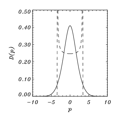
The above general derivation [61] allows however to study any arbitrary distribution. Let us carry on here the calculation of the diffusion coefficient for the Vlasov-stable water bag distribution (293). It has an interesting behavior, since the dielectric response has zeroes on the real axis, contrary to any even distributions strictly decreasing for positive values of the frequency . One gets
| (337) |
which is also plotted in Fig. 36. One can obtain similar results for -exponential distributions (294) (see Ref. [110]) or power-law tails distributions (295).
V.2.3 Long-range temporal correlations and diffusion
Since the Fokker-Planck equation for the single particle distribution function has a variable diffusion coefficient, the relaxation towards the Boltzmann distribution can be slowed down, especially if the diffusion coefficient decreases rapidly with momentum. It is thus important to study this Fokker-Planck equation for different distribution functions of the bath. A similar study was earlier performed for 2D vortices in Ref. [92]. One consequence is that velocity correlation functions can decrease algebraically with time instead of exponentially, a behavior which might lead to anomalous diffusion as we will show below.
By introducing the appropriate change of variable , defined by , and the associated distribution function , defined by , one can map [239, 149, 242, 61, 106] the Fokker-Planck equation (335) to the constant diffusion coefficient Fokker-Planck equation
| (338) |
where the potential is given by
| (339) |
Using the property , that implies, by Eq. (333), that , one gets . From this, one derives that for many classes of distribution functions , the potential is asymptotically equivalent to a logarithm. In fact, we have
| (340) |
with if decreases to zero more rapidly than algebraically for large , and if decreases to zero algebraically; more precisely, if decays at large as . For weakly confining potentials , i.e., when and thus , Eq. (338) has a non-normalizable ground state. The example of the heat equation, which corresponds to , describes a diffusive process leading to an asymptotic self-similar evolution. In such a case, the spectrum of the Fokker-Planck equation is purely continuous. By contrast, a strongly confining potential (for instance, the Ornstein-Ulhenbeck process with a quadratic potential) would lead to exponentially decreasing distributions and autocorrelation functions, linked to the existence in the spectrum of a gap above the ground state. The logarithmic potential (340) is a limiting case between the two behaviors. The normalizable ground state is unique and coincides with the bottom of the continuous spectrum. The absence of a gap forbids a priori any exponential relaxation. To illustrate this result, we evaluate the asymptotic behavior explicitly in two cases.
- •
Let us first consider distribution functions with fast (more than algebraically) decreasing tails so that
(341) which includes not only the Gaussian and exponential tails , but also stretched-exponential ones with any arbitrary positive exponent . From the change of variable , asymptotic analysis leads to and to . These estimates are sufficient (see Ref. [61] for details) to evaluate the long time behavior of the momentum autocorrelation function
(342) which proves the existence of long-range temporal momentum autocorrelation for all values of , and therefore also in the case of Boltzmann equilibrium, .
- •
Let us now consider a distribution function with algebraic tails
(343) In this case, one has and the asymptotic behavior (340) with, as we said, . We consider only cases where , to ensure that the second moment of the distribution (i.e., the average kinetic energy) does exist. For one has that . The result for the momentum autocorrelation function is
(344) which characterizes an algebraic asymptotic behavior.
From the momenta autocorrelation, one usually derives the angle diffusion where is defined via the Kubo formula
| (345) |
However, since the exponent is larger than , the asymptotic result (344) shows that the integral (345) diverges. The asymptotic result (342) leads also to a divergent integral, although less singular. It is thus natural to expect anomalous diffusion for the angles. This extremely small anomaly (logarithmic) for distribution functions with Gaussian or stretched exponential tails induced difficulties to detect numerically anomalous diffusion [217, 314].
Note that, generalizing the theory of Potapenko et al. [268], Chavanis and Lemou [105] studied how the structure and the progression of the distribution function tails, also called fronts, depends on the behavior of the diffusion coefficient for large velocities. They showed that the progression of the front is extremely slow (logarithmic) in that case so that the convergence towards the equilibrium state is peculiar.
Using the time rescaling , which introduces a factor , the angles diffusion can be rewritten as
| (346) | |||||
| (347) |
in which the new variable has been introduced to take advantage of the division of the square domain into two isoscale triangles corresponding to and . In the quasi-stationary states, the integrand does not depend on (the QSS evolves on a time scale much larger than ) and hence diffusion can be simplified [314] as
| (348) |
A distribution with power law tails (343) will therefore correspond to
| (349) |
A comparison of this predicted [61] anomalous diffusion for angles with direct numerical computation of the HMF dynamics is a tough task because of the scaling with of the time dependence of the autocorrelation function. However, it has been recently confirmed by numerical simulations in Ref. [317]. For the stable case () with power-law tails (), the theory predicts that the correlation function decays algebraically with the exponent (see Eq. (344)). Figure 37(a) shows that the theoretical prediction agrees well with numerical computations. The expression (349) can be rewritten in that case as : Figure 37(b), in which the four curves for the four different values of almost collapse, attests also the validity of this prediction. This is a clear example of anomalous diffusion.


For the stretched exponential distribution function (341), one ends up with
| (350) |
As for power law tails, the diffusion is again anomalous, although with a logarithmically small anomaly. Consequently, the anomalous diffusion for angles also occurs for the Gaussian distribution which corresponds to the special case . This weak anomalous diffusion, i.e. normal diffusion with logarithmic corrections, has also been confirmed [317]. Since Gaussian distributions correspond to equilibrium distributions in the microcanonical and the canonical ensembles, it is important to realize that anomalous diffusion might thus be encountered for both equilibrium and out-of-equilibrium initial conditions. An analogous behavior has been observed for point vortices [94, 106].
V.2.4 Lynden-Bell’s entropy
In subsection V.2.1 we have discussed in detail, focusing on the HMF model, the two-stage relaxation process that is often observed in systems with long-range interactions. It has been indeed realized, beginning with a seminal paper by Hénon [174] on globular clusters, that the dynamical evolution is divided in two well separated phases. A first phase, called dynamical mixing, where an initial fast (violent) evolution leads to a quasi-stationary state, and a second phase, called relaxation phase, where “collisions” have the cumulative effect to drive the systems towards statistical equilibrium. If the number of particles is large, the two phases are well separated in time. It was also observed that the quasi-stationary state was strongly dependent on the initial condition [174]. In subsection V.1.4 we have discussed the existence of stationary stable and unstable one-particle distributions for the Vlasov equation and we have presented (subsection V.2.1) the interpretation of quasi-stationary states in terms of “attractive” Vlasov equilibria. A statistical approach that explains the existence of Vlasov equilibria has been proposed long ago by Lynden-Bell [230]. He begins by remarking that Vlasov equation, which represents the evolution of an incompressible fluid, obeys Liouville theorem in six dimensions. We will here restrict to a two-dimensional phase space for simplicity. This implies that the “mass” of phase elements between and is conserved (remind that is the one-particle distribution function). If we discretize the one-particle distribution function into a set of quantized levels , , this means that the area corresponding to the -th level is a constant of the motion. In the limit of a continuous distribution of levels, one obtains an infinity of conservation laws. It is easy to prove that this implies that any functional of the form is conserved: these functionals are called Casimirs. For instance, Gibbs entropy is a particular Casimir: . This specifically implies that, in terms of the fine grained one-particle distribution, Gibbs entropy cannot increase. Let us then define a coarse grained distribution
| (351) |
where is the probability of finding level in the phase-space macrocell . Obtaining this probability directly from the microscopic dynamics is an extremely difficult problem, and its solution would constitute a significant step forward in the understanding of the nature of quasi-stationary states. Lynden-Bell’s proposal is to evaluate by using a sort of “Boltzmann principle” [274, 275, 276, 243, 141]. The evaluation of can be done for any number of levels , but to make the calculation simpler, let us approximate the one-particle distribution with only two levels and (the case with many levels has been treated in Refs. [230, 97]). Alternatively, one can consider a fine-grained distribution function which, at , has only two levels: these are called water-bags in astrophysics and plasma physics. The exact time evolution of the water-bag is such that the shape of the area occupied by the Vlasov “fluid” with level is deformed, stretched and folded due to the hyperbolicity originated by the nonlinear dynamics of the Vlasov equation (see e.g. Fig. 2 in Ref. [230]). However, due to Liouville’s theorem, this area is conserved. Let us divide each macrocell into microcells of volume and consider a microscopic configuration in which the -th macrocell is occupied by microcells with level and with level zero. The total number of occupied microcells is , such that the total mass is . This latter is also equal to the normalization of the fine grained distribution . The occupied microcells are first placed into macrocells. There are ways to do this. Within the -th cell, one can distribute the first of the occupied microcells in ways, the second in and so on. The number of ways of assigning the occupied microcells is thus . Then, the total number of microstates compatible with the macrostate where microcells are occupied in macrocell is given by the product of these two factors
| (352) |
The first factor is calculated exactly as for Boltzmann gas [183], because the occupied microcells are distinguishable, while the second factor reminds Fermi-Dirac statistics and derives from an exclusion principle, which is a consequence of fluid incompressibility: one microcell cannot be occupied more than once by a fluid element of level . Apart from this latter constraint, fluid microcells are let to distribute freely among the different macrocells: this corresponds to making an assumption of ergodicity. This doesn’t happen for the true Vlasov dynamics and is sometimes referred to as the hypothesis of efficient mixing. Indeed, it has been found that dynamical effects can hinder mixing [15, 18, 22, 223, 224, 65, 95]. Using Stirling’s approximation and expressing in terms of the average probability to find level in cell , , one obtains, neglecting an additive constant,
| (353) |
which can also be rewritten in terms of the coarse grained distribution function, . Taking the continuum limit , one finally gets
| (354) |
Following the standard procedure, inspired by large deviation theory [300], one then maximizes subject to the constraint of conserving energy , mass and other global invariants like momentum (or angular momentum for higher dimensions).
Historically, the first applications of Lynden-Bell’s ideas encountered both confirmations and failures [180, 119, 176, 318], although the crucial point of necessarily performing simulations with a large number of particles was never clearly addressed, due to computer time limitations. Very recently, a careful analysis of the one-dimensional self-gravitating sheet model has shown that Lynden-Bell statistics applies for initial data with virial ratio close to unity [315]. A statistical theory similar to Lynden-Bell’s was independently developed for the Euler equation [245, 275, 277] and, later on, the deep analogy between the Vlasov-Poisson system and the Euler equation was for the first time clearly stressed in Ref. [109]. This approach was then used in the context of mean-field models in Refs. [39, 16], with an application to the Colson-Bonifacio model of the Free Electron Laser (see subsection IV.5.6). As already discussed in section V.2.1, the presence of quasi-stationary states for the HMF model was recognized and characterized numerically in Ref. [316]. Lynden-Bell’s theory was then shown to predict the main features of the one-particle distribution function of quasi-stationary states of the HMF model in Ref. [17]. Let’s finish this subsection by discussing in some detail this latter result, which clearly shows the power of Lynden-Bell’s approach.
Let us first recall the Vlasov equation for the HMF model
| (355) |
where is the fine grained one-particle distribution function and
| (356) | |||||
| (357) | |||||
| (358) |
The globally conserved quantities are energy
| (359) |
and momentum
| (360) |
As for the initial distribution, we consider a water bag with rectangular shape in the plane. The distribution takes only two distinct values, namely , if the angles (velocities) lie within an interval centered around zero and of half-width (), and zero otherwise (“mass” is normalized to one and momentum is zero). There is a one to one relation between the parameters and and the initial values of magnetization and energy
| (361) |
While and are constants of the motion, magnetization evolves with time. Lynden-Bell’s maximum entropy principle is then defined by the following constrained variational problem
| (362) |
The problem is solved by introducing three Lagrange multipliers , and for energy, momentum and mass normalization. This leads to the following analytical form of the distribution
| (363) |
This distribution differs from the Boltzmann-Gibbs one because of the “fermionic” denominator. Inserting expression (363) into the energy, momentum and normalization constraints and using the definition of the magnetization, it can be straightforwardly shown that the momentum multiplier vanishes, . Moreover, defining and , yields the following system of implicit equations in the unknowns , , and
| (364) | |||||
| (365) | |||||
| (366) | |||||
| (367) |
with and . This system of equations can be solved numerically and, given the parameters that fix the initial conditions, i.e. energy, momentum and , univocally determines the values of the Lagrange multipliers and , the values of and where Lynden-Bell’s entropy is extremal and, finally, the distribution in formula (363) itself, with no adjustable parameter. For , the maximum entropy state has zero magnetization for , a value at which Lynden-Bell’s theory predicts a second order phase transitions [17, 18, 100]. Interpreting as the distribution in the quasi-stationary state (QSS), we obtain in this case
| (368) |
with and to be determined from the knowledge of . Velocity profiles predicted by (368) are displayed in Fig. 38 for different values of the initial magnetization.

Although not a single free parameter is used, one finds an excellent qualitative agreement. The presence of two symmetric bumps in the velocity distributions is not predicted by Lynden-Bell’s theory and is a consequence of a collective phenomenon which leads to the formation of two clusters in the plane. This is shown by the direct simulation of the Vlasov equation (355) presented in Fig. 39. The bumps represent an intrinsic peculiarity of QSS and have been characterized dynamically in Ref. [22].
More recently, other authors have obtained similar encouraging results for Lynden-Bell’s theory in a model of non-neutral plasma [223] and for radially symmetric solutions of a self-gravitating system [224]. They also find that, when dynamical effects lead to collective oscillations of the mean-field, Lynden-Bell’s theory shows a disagreement with numerical data and propose a modification of the theory. Work along this line is in progress.

The theoretical approach proposed by Lynden-Bell [230] allows to predict the presence of a phase transition line in the and in the control parameter planes [18, 101]. At equilibrium the At equilibrium the phase transition does not depend on the choice of and is located at . On the contrary, in the out-of-equilibrium QSS the phase transition line is located at smaller energies joining the transition points [316] and in the plane. Moreover the phase transition changes from first to second order. These latter results are resumed in Ref. [104].
The Lynden-Bell approach turns out to be a good way to attack the problem of quasi-stationary states. It gives predictions for both averages and distributions functions which compare quite well with numerical simulations. When the approach fails to describe detailed features, they are viable ways of modifying it taking into account dynamical properties.
VI Generalization to non mean-field models
Although substantial progress has been done recently in the understanding of long-range interactions, the hardest questions about physical systems where the interactions weakly decay with the distance, and also shows singularities at short distances, remain open (see the introductory section III). In section IV, we have shown how simple mean-field models, that are explicitly solvable in both the canonical and the microcanonical ensemble, already show several features previously encountered in gravitational systems, e.g. negative specific heat. These simple models also display peculiar out-of-equilibrium dynamical effects, like the presence of quasi-stationary states, which resemble those found for realistic systems, see section V.
In this section, we make a little step in the direction of the study of Hamiltonians that are not fully mean-field. In subsection VI.1 we introduce, for both a mean-field Ising and an XY model, a nearest-neighbour interaction term. We show that the phase diagram in canonical and microcanonical ensembles preserves the features of non equivalence found for pure mean-field Hamiltonians. In particular, we mention the non coincidence of the microcanonical and canonical tricritical points and the presence of negative specific heat. In subsection VI.2, we consider an Ising model in one dimension with weakly decaying coupling and a modification of the HMF model which includes a coupling with the same properties. For both models, we show that the mean-field properties extend to the weakly decaying case and that one can obtain analytically the free energy and the entropy. Since the corresponding mean-field limit of both models shows ensemble equivalence, this property persists also for such models. In subsection VI.2.3, we show the analytical solution in both the canonical and microcanical ensembles of a self-gravitating system of particles moving in one dimension. The phase diagram is different in the two ensembles and show all features of ensemble inequivalence. In an appropriate limit, the model reduces to the HMF model and therefore ensemble inequivalence can be turned off by varying a parameter. Finally, in subsection VI.2.4, we conclude with a summary of a very recent result concerning a spin system with dipolar interactions whose Hamiltonian can be reduced in appropriate limits to that of the XY model with nearest neighbour and mean-field interactions presented in subsection VI.1. This result opens the possibility to verify experimentally some of the striking and counterintuitive features of long-range interactions.
VI.1 Systems with short- and long-range interactions: the transfer integral method
In this subsection, we will present both the canonical and the microcanonical solutions of an Ising model and of an XY model with nearest neighbour and mean-field interactions. We will obtain the phase diagram in both ensembles. All the features of mean-field models discussed in Sec. IV will appear again in this context: ensemble inequivalence, negative specific heat, temperature jumps, ergodicity breaking. This shows that the addition of a short-range term to a long-range Hamiltonian does not remove the interesting behaviors described before. For what concerns methodological aspects, the use of transfer integral combined with the Hubbard-Stratonovich transformations and the min-max method allows us to treat both models with discrete and continuous variable. The models we will consider are defined on a one-dimensional lattice (indeed a ring because of the periodic boundary conditions), but there is no reason of principle that forbid to extend the calculation to strip and bar geometries.
VI.1.1 Ising model
Introduction
Nagle introduced an interesting Ising model combining long- with short-range interactions [250]. Further elaborations of the model were proposed by Khardar [194, 195]. The Hamiltonian is
| (369) |
where . In this one-dimensional spin chains, the first term has an infinite range and is the typical one of the Curie-Weiss Hamiltonian (1). This term is responsible for the non additive properties of the model, see Sec. II.1. Note that the prefactor present in Hamiltonian (1) has been set to one by an appropriate renormalization of the energy. There is no loss of generality, since only the ferromagnetic case will be considered. On the contrary, the second term of (369) corresponds to an interaction between nearest neighbors along a one-dimensional lattice (periodic boundary conditions are chosen). The coupling constant might be either positive or negative.
The ferromagnetic state with all spins up () or down () has a negative energy . For the antiferromagnetic state with alternate signs of nearest neighbour spins, the first term of (369) gives a vanishing contribution to the energy and the energy is . At , one can determine if the model has a phase transition at some value of by comparing the energy of the ferromagnetic state with that of the antiferromagnetic one, since only the energy term of the free energy matters. Hence, by imposing one gets the phase transition value at which a discontinuity of the order parameter is found, from to . Therefore the transition is first order.
.
For non zero temperature, one has to take into account the entropic term of the free energy, which measures disorder. When the coupling constant vanishes, one fully recovers the Curie-Weiss Hamiltonian (1), which exhibits a second order phase transition at . One therefore expects that the phase diagram displays a transition line which is first order at low and second order at high (see Fig. 40). The transition line separates a ferromagnetic from a paramagnetic state, although exactly at and the state is antiferromagnetic. Let us now determine analytically this transition line in both the canonical and the microcanonical ensemble.
The solution in the canonical ensemble
The phase diagram has been studied in the canonical ensemble by Nagle [250] and Khardar [194, 195]. The partition function is
| (370) |
To get rid of the quadratic term, we use the Hubbard-Stratonovich transformation
| (371) |
so that the partition function (370) can be rewritten as
| (372) | |||||
| (373) |
The free energy can be written as
| (374) |
where is the free energy of the nearest-neighbor Ising model with an external field . Such an expression can be easily derived using the transfer matrix [211, 183, 194]. By an easy calculation, we find where the two eigenvalues of the transfer matrix are
| (375) |
As for all values of , only the larger eigenvalue is relevant in the limit . One thus finally gets
| (376) |
which is shown in Fig. 41 for different values of the inverse temperature and for two values of the nearest-neighbor coupling .


In the large -limit, the application of the saddle point method to Eq. (373) finally leads to the free energy, which is obtained by taking the value of which minimizes in formula (376).
From the knowledge of the free energy, as anticipated, one gets either a second or a first order phase transition depending on the value of the coupling constant . As usual, the expansion of in power of is the appropriate procedure to define the critical lines and points. One gets here
| (377) |
The critical point of the second order transition is obtained for each by computing the value at which the quadratic term of the expansion (377) vanishes provided the coefficient of the fourth order term is positive, obtaining . When also the fourth order coefficient vanishes, one gets the canonical tricritical point (CTP) . The first order line is obtained numerically by requiring that , where is the further local minimum of . Figure 42 represents the phase diagram in both the canonical and the microcanonical ensembles. The features of this phase diagram are very close to those of the BEG model (see Fig. 14) and of the generalized HMF (see Fig.23). We will comment them below, after having obtained the solution in the microcanonical ensemble [248].

The solution in the microcanonical ensemble
In the microcanonical ensemble, a simple counting method has been recently proposed [248]. The magnetization can be rewritten as by introducing the number of spins up, , and of spins down, . The first term of the Hamiltonian (369) can be straightforwardly rewritten as . As two identical neighboring spins would not contribute to the second term of Hamiltonian (369) ( being equal to zero) while two different ones would give a contribution equal to , the total contribution of the second term is , where is the number of “kinks” in the chain, i.e. links between two neighboring spins of opposite signs.
For a chain of spins, the number of microstates corresponding to an energy can be written as
| (378) |
The formula is derived by taking into account that we have to distribute spins among groups and among the remaining . Each of these distributions gives a binomial term, and, since they are independent, the total number of states is the product of the two binomials. The expression is not exact because we are on a ring, but corrections are however of order and do not affect the entropy. A slight correction to formula (378) is present for small , and , and all these numbers should be indeed reduced by a unity.
Introducing , and , one thus finally gets the entropy
| (379) | |||||
which is shown in Fig. 43 for different values of the energy and for two values of the nearest-neighbor coupling .


In the large -limit, the last step is to maximize the entropy with respect to the magnetization , leading to the final entropy , where is the equilibrium value. As anticipated, one gets either a second or a first order phase transition depending on the value of the coupling constant . As usual, and analogously to what has been done in the canonical ensemble, the expansion of in power of is the appropriate procedure to define the critical lines and points. One gets here
| (380) |
with the paramagnetic zero magnetization entropy
| (381) |
and the expansion coefficients
| (382) | |||||
| (383) |
Using these expression, it is straightforward to find the second order phase transition line by requiring that (), finding , which is the same equation found for the canonical ensemble. Again, as far as second order phase transitions are concerned, the two ensembles are equivalent. The tricritical point is obtained by the condition ), which gives and , which is close but definitely different from and . The microcanonical first order phase transition line is obtained numerically by equating the entropies of the ferromagnetic and paramagnetic phases. At a given transition energy, there are two temperatures, thus giving a it temperature jump as for the BEG and the generalized HMF model. Similarly to mean-field models, also this model exhibits a region of negative specific heat when the phase transition is first order in the canonical ensemble.
Equilibrium dynamics: breaking of ergodicity
Model (369) exhibits breaking of ergodicity, as shown in Ref. [248]. In order to reveal the dynamical consequences of this effect, one has to define a microcanonical dynamics. An appropriate one is given by the Creutz algorithm [122], which probes the microstates of the system with energy lower or equal to the energy . Indeed, there are two definitions of the microcanonical ensemble, that become equivalent in the thermodynamic limit. In the first one, only states contained on an energy shell are counted (this is the definition we used throughout this review); in the second one all the phase-space volume contained within the energy hypersurface is considered [183]. Creutz algorithm is based on this second definition.
The algorithm is implemented by adding an auxiliary variable, called a demon, which has the following properties. One initiates the procedure with the demon at zero energy, while the system has an energy . One then attempts to flip a spin. The move is accepted if it corresponds to an energy decrease and the excess energy is given to the demon. One then attempts to flip another spin. If the flip decreases the energy, it is accepted, while if it increases the total energy, it is accepted only if the needed energy can be withdrawn from the demon energy. Demon serves really as a bank with deposit and withdrawn: however, the total energy of the “bank” is always non negative (clearly different from typical banks in the 21st century!).
Creutz dynamics can be used to test the predictions on breaking of ergodicity discussed in Sec.IV.5.4. Indeed, as it is already apparent in Fig. 43, not all magnetization values are accessible in certain regions of the plane, which manifests itself in the gaps of the entropy curves shown in Fig.43. This property is in turn a consequence of the non convexity of the space of thermodynamic parameters (see Sec. II.3)
To demonstrate ergodicity breaking, we show in Fig. 44 the time evolution of the magnetization in two cases: in the first case, where the whole magnetization interval is accessible, one clearly see switches between the metastable state and two stable symmetric magnetized states. On the contrary, in the second example, the metastable state belongs to an interval which is disconnected from the stable one (see the inset for the corresponding entropy curve). The dynamics maintains the system either in the stable or in the metastable interval, depending only on the initial condition. The system is unable to jump to the other interval even when the latter is more stable.
Similar results had been obtained using Hamiltonian dynamics for the generalized HMF model, see Fig. 29.

VI.1.2 XY model
Introduction
In this subsection we study a generalization of the HMF model, in which the Hamiltonian, besides the mean-field interaction, has a nearest neighbour interaction between rotators. The presence of such a term requires that we specify the properties of the lattice where the model is defined. As in subsection VI.1.1, we study a one-dimensional lattice with a ring geometry; the first property allows the use of the transfer integral technique, while the second property, equivalent to the introduction of periodic boundary conditions, is convenient for the calculations, but it is irrelevant in the thermodynamic limit.
The model has been introduced in Ref. [76], and its Hamiltonian is given by
| (384) |
with . The parameter is the coupling constant of the nearest-neighbour interaction. For , the Hamiltonian reduces to the HMF model, that has a second order phase transition at . The similarities of this model with the Ising model studied in the previous subsection are clear: there is a mean-field interaction and a nearest neighbour interaction. However, there is also a kinetic energy term, which allows to define a Hamiltonian dynamics. Also in this case the interesting properties are found for . Let us first locate the first order transition at . This is done, as for the Ising case, comparing the energy per particle of the fully magnetized state with that of the staggered non magnetic state. The energy density of the former is , while that of the latter is . The magnetized state is therefore favoured for . Qualitatively, it is the same phase diagram as the one observed in Fig. 40.
Solutions in the canonical and microcanonical ensembles
We adopt the min-max procedure, described in subsection IV.4.4. We remind that, in this procedure, once an expression for the canonical partition function has been obtained in the form of Eq. (155), not only can we compute the canonical free energy by the minimization defined in Eq. (156), but we can also obtain the microcanonical entropy by Eq. (160).
Let us first derive the canonical partition function. As for the HMF model, we use the Hubbard-Stratonovich transformation. The model shares with the HMF model the invariance under global rotations, therefore the spontaneous magnetization is defined only in modulus, while there is degeneracy with respect to its direction. We can exploit this fact to simplify slightly the computation; namely, we assume from the beginning that the saddle point value of the variable in Eq. (130) is . The spontaneous magnetization is in the direction of the -axis, but this will not cause any loss of generality. We therefore obtain
| (385) | |||||
The integral over the ’s is performed applying the transfer integral method. For our one-dimensional geometry this is given by
| (386) |
where is the -th eigenvalue of the symmetric integral operator
| (387) |
In the thermodynamic limit, only the largest eigenvalue will contribute to the partition function. This eigenvalue can be computed numerically by a suitable discretization of the integral operator (387). The rescaled free energy is
| (388) |
with
| (389) |
where we have not explicitly written the dependence of and .
Accordingly to the min-max procedure, the microcanonical entropy is given by
| (390) |
with
| (391) |
Again the dependence of and on has not been explicitly written. The expressions (389) and (391) are used to study canonical and microcanonical thermodynamic phase diagrams, respectively, and then to check if there is ensemble inequivalence. As for the Ising case, to obtain the critical lines on the plane, one has to expand and in powers of . The power expansion of can be obtained explicitly as a function of modified Bessel functions. We will avoid here the details of the calculation leading to the final result.
Taking into account that our system is invariant under the symmetry , the expansion of will have only even powers. Let us write explicitly the dependence of the expansion coefficients
| (392) |
The canonical second order transition line in the plane is determined by
| (393) |
Inserting this expansion in the first equality in Eq. (391) and minimizing with respect to , one obtains
| (394) |
where the prime denotes derivation with respect to . This equation gives an expansion of the form
| (395) |
Using this expression, we obtain the expansion of the form
| (396) |
where
| (397) | |||||
| (398) | |||||
| (399) | |||||
The microcanonical second order transition line is determined by
| (400) |
Now we can use the following equalities, that are obtained by inserting back (395) into (394)
| (401) | |||||
| (402) |
Equation (401) implies that is the temperature on the second order transition line. One obtains
| (403) | |||||
Therefore, the microcanonical second order transition line is determined by
| (404) |
The concavity of implies that, again on the critical line, (This is valid in models where parity with respect to implies that for ). Comparing Eqs. (393) and (404), and taking into account the last observation, we see that, as we expected from the general discussion about ensemble equivalence at the end of subsection IV.1.3, the points belonging to the canonical second order transition line also belong to the microcanonical one. The microcanonical line, however, goes beyond and includes more points, as we have already seen in several models, since by continuity the inequality in (404) is satisfied also for some points where .
The study of the canonical and microcanonical critical lines involves the analytic determination of , which, in the limit , can be performed using perturbation theory for Hermitian operators [228]. For both ensembles, one gets
| (405) |
where and are modified Bessel functions. The canonical tricritical point turns out to be and , while microcanonical tricritical point is at and . In Fig. 45, we plot the relevant part of the phase diagram on the plane. As commented above, it is shown how the microcanonical critical line (ending at the microcanonical tricritical point MTP) extends beyond the canonical critical line, which ends at the canonical tricritical point CTP.

Ergodicity breaking
We here prove that model (384) shows ergodicity breaking, similarly to the Ising long- plus short-range model. Let us first study separately the bounds of the short-range term
| (406) |
The study of maxima and minima of this term can be reduced to those configurations where the spins are aligned parallel or antiparallel to a given direction. There is no loss of generality, due to rotational symmetry, to then choose this direction as the -axis. Therefore, only the component of is non zero and in the following we will restrict to . It turns out that, in the thermodynamic limit, both extrema are attained with a fraction of rotators parallel to the -axis and a fraction antiparallel to the -axis, for all given values of . The maximum is and is achieved when the parallel rotators and the antiparallel rotators are grouped in two separated blocks. The minimum , is instead attained when the antiparallel rotators are all isolated, which is possible since we are considering .
Now we have to distinguish the two cases and . In the positive case, the minimum of this contribution to the energy density is (thus actually independent of ), while in the negative case it is . We obtain the minimum of the total potential energy per particle just by adding . This is actually the minimum of the total energy per particle , since the kinetic energy is positive definite. We finally obtain that the minimum of the energy per particle is
| (407) |
for , and
| (408) |
for . Plotting the two functions and we will find the accessible values for a given energy . The functions are plotted in Fig. 46 for two representative values: and . For positive , we see that below the energy the system cannot have all magnetizations, and values of near are inaccessible. We note however that the region of accessible values of , for any energy, is connected; therefore there is no ergodicity breaking. Nevertheless, we remark that the accessible region in the plane is not convex, as it can happen only for long-range interactions. For negative , we note instead, that for a given energy interval ( for and for ), the attainable values of are separated in two disconnected regions. Therefore for we have breaking of ergodicity.

VI.2 Weakly decaying interactions
All the models that have been considered in previous sections have an infinite range term in the Hamiltonian. This undoubtly limits the applicability of our analysis to realistic physical systems, where interactions decay with the distance. We present below four models of this kind which are direct generalizations of models presented above and represent a step forward in the study of long-range weakly decaying interactions. Some of the models are exactly solvable and reproduce features of the phenomenology observed for infinite range systems (ensemble inequivalence, negative specific heat, ergodicity breaking, etc.).
VI.2.1 -Ising model
Let us consider the one-dimensional -Ising Hamiltonian
| (409) |
where and spins sit on a one-dimensional lattice with either free or periodic boundary conditions (in the latter case, is the minimal distance along the ring). The prefactor is introduced in order to have an extensive energy as explained in Sec. II.1. This model has been first introduced by Dyson [138] and studied for the “integrable” case, , in the canonical ensemble without the prefactor. We show here that it is possible to obtain an exact microcanonical solution using large deviation theory when [32, 43, 37]. Moreover, the study of this model gives also the opportunity to emphasize the important role played by boundary conditions when the interactions are long-range.
We adopt the same scheme described in section IV.5 to obtain the solution of model (409). The method can be generalized to lattices of higher dimension.
In the first step, the Hamiltonian is rewritten in terms of global variables by introducing a coarse-graining. Let us divide the lattice in boxes, each with sites, and let us introduce the average magnetization in each box , . In the limit , , , the magnetization becomes a continuous function of the interval. After a long but straightforward calculation, described in Ref. [37], it is possible to express as a functional of
| (410) |
where
| (411) |
The estimation is uniform on all configurations.
In the second step, we evaluate the probability to get a given magnetization in the -th box from all a priori equiprobable microscopic configurations. This probability obeys a local large deviation principle , with
| (412) |
Since the microscopic random variables in the different boxes are independent and no global constraints has been imposed, the probability of the full global variable can be expressed in a factorized form as
| (413) | |||||
| (414) | |||||
| (415) |
where is the entropy functional associated to the global variable . Large deviation techniques rigorously justify these calculations [57], proving that entropy is proportional to , also in the presence of long-range interactions. This result is independent of the specific model considered.
In the third step, we formulate the variational problem in the microcanonical ensemble to get the entropy
| (416) |
Let us remark that this optimization problem has to be solved in a functional space. In general, this has to be done numerically, taking into account boundary conditions. In the case of free boundary conditions, the only available solutions are numerical. An example of a maximal entropy magnetization profile obtained for free boundary conditions is shown in Fig. 47 for different values of . The profile become more inhomogeneous when increasing (for one recovers the mean-field result with a homogeneous profile).

In the following, we will treat the periodic boundary conditions case, for which analytical result can be obtained. Both entropy and free energy can be obtained in analytical form for homogeneous magnetization profiles, which have been shown to be locally stable in both the high-temperature and the low-temperature phase [37]. It has indeed been proven that for there is a unique global maximum of , corresponding to a constant zero magnetization profile. The variational problem (416), where is defined in Eqs. (412), (414) and (415), leads to the consistency equation
| (417) |
where is a Lagrange multiplier. For , we restrict ourselves to constant magnetization profiles, which are locally stable, i.e. close non constant profiles have a smaller entropy. In this case, using the relations and one can obtain the magnetization vs. energy curve , see Fig. 48(a). Moreover, fixing the energy implies fixing the magnetization and, consequently, the Lagrange multiplier in Eq. (417). Expressing the magnetization in terms of the energy in the entropy formula (416) allows us to derive the caloric curve, see Fig. 48(b) (solid line). The limit temperature (dotted line) is attained at zero magnetization, which is a boundary point.

In the canonical ensemble, one has to solve the variational problem (195). This leads to exactly the same consistency equation (417), where the Lagrange multiplier is replaced by the inverse temperature . Solving this consistency equation for , one finds a zero magnetization for and a non vanishing one for . One can also derive the canonical caloric curve, which is reported in Fig. 48(b) and superposes to the microcanonical caloric curve from down to while it is represented by the dashed line for . It follows that in the region , the two ensembles are not equivalent. In this case, a single microcanonical state at corresponds to many canonical states with canonical inverse temperatures in the range . Thus, in such a case, the canonical inverse temperature is not equal to the microcanonical one. In the microcanonical ensemble, the full high temperature region is absent and, therefore, no phase transition is present or, in other terms, the phase transition is at the boundary of the accessible energy values. The entropy is always concave, hence no inequivalence can be present in the allowed energy range, apart from the boundaries. This situation is often called partial equivalence [141, 300, 83]. Partial equivalence persists for all values below one, and is removed only for when and : the phase transition is not present in both ensembles and the system is always in its magnetized phase. The main drawback of this analysis is the difficulty to obtain analytical solutions of Eq. (417) for non constant magnetization profiles, which is the typical situation when boundary conditions are not periodic.
VI.2.2 -HMF model
Let us consider now a generalization of the HMF model (126) which has been originally proposed in Ref. [8, 293]. The interaction between two rotators has the same form as in the original model, but the coupling constant is a weakly decaying function of the distance between the two lattice sites where the rotators sit. Note that we consider the lattice in general dimension . In Ref. [75], the generalized case of -vector spin models has been analyzed, including the HMF model (for ) and the Ising spins (for ). Only periodic boundary conditions have been considered, as we will do here.
The Hamiltonian of the -HMF model is
| (418) |
where is the minimal distance between lattice sites and (minimal distance convention in periodic boundary conditions). We consider here cases for which the exponent , determining the decay with distance of the coupling constant between rotators, is less than the spatial dimension , so that the system is long-range as shown in Sec. II.2. The prefactor is introduced in order to have an extensive energy as explained in Sec. II.1. We show below that, in any spatial dimension and for each , the thermodynamics of this model is the same as that of the HMF model; in particular, there is a second order phase transition at the inverse temperature .
Let us introduce the matrix of the coupling constants . Since the diagonal elements of this matrix are not defined, we assign to them the common arbitrary value . The prefactor is
| (419) |
that does not depend on , because we adopt the minimal distance convention for . It is clear that in the thermodynamic limit , the prefactor behaves as . The arbitrary parameter , which appears only in , becomes negligible in thermodynamic limit. Its introduction is however useful for the computation, as it will become clear.
The most relevant steps of the solution in the canonical ensemble (we refer the reader to Ref. [75] for details) can be obtained starting from the partition function
| (420) | |||||
| (421) |
where we have introduced the matrix and used the property . In order to use the Hubbard-Stratonovich transformation, one diagonalizes the expression in the second exponential. Denoting by the symmetric matrix with elements , and by the unitary matrix that reduces to its diagonal form , one gets
| (422) |
where the quantities are the real eigenvalues of the matrix , and . An analogous expression holds for the sum with the sines in Eq. (421). In order to express using the Hubbard-Stratonovich transformation, the eigenvalues must be positive. By choosing a sufficiently large value of , but in any case of order , all eigenvalues are positive. One can therefore write
| (423) | |||||
| (424) |
In this -dimensional Hubbard-Stratonovich transformation, we have used that , we have introduced the unitary change of integration variables defined by and we have indicated with the inverse matrix of . Using the analogous expression for the term with the sines, we arrive, after performing the integration over the angles , to the following expression for the partition function
| (425) | |||||
This integral can be computed using the saddle point method, since most eigenvalues vanish in the thermodynamic limit [75]. Introducing , the stationary points are solutions of the following consistency equations
| (426) | |||||
| (427) |
which, after inversion with respect to , become
| (428) | |||||
| (429) |
Let us first look for homogeneous solutions, i.e., for solutions in that do not depend on . The previous system reduces to the following pair of equations for and
| (430) |
where we have used that for each . By expressing and , we see that these two equations determine only the modulus , leaving the angle undetermined. They thus reduce to a single equation for the modulus
| (431) |
This equation, after the change of variable , coincides with Eq. (134) of the HMF model.
In order for this homogeneous stationary point to be the relevant one for the evaluation of the integral in Eq. (425), it is necessary that the exponential has an absolute maximum at this stationary point. One can easily show that the homogeneous stationary point is a local maximum [75]. Here, we will directly prove that it is also a global maximum with respect to any other possible inhomogeneous stationary point.
Let us then go back to Eqs. (428) and (429) and suppose that they have inhomogeneous solution, considering as a first case a solution with different values for the moduli . If is the site with the largest modulus , let us choose the -axis of the XY rotators such that and . Then one can write
| (432) | |||||
| (433) |
where use has been made of the monotonicity of the function . We emphasize that the last inequality is strict since, by hypothesis, not all moduli are equal. From the properties of the function , it follows from the last inequality that also the largest modulus of this inhomogeneous stationary point is smaller than that of the homogeneous solution. One gets the same conclusion for a possible stationary point with all equal moduli but with different directions; in that case inequality (433) becomes an equality, but inequality (433) is strict. The proof is completed by showing that the exponent in Eq. (425), if computed at a stationary point, has a positive derivative with the respect the moduli of the stationary point. In fact, it can be easily shown that at a stationary point the exponent in Eq. (425), let us call it , can be written as a function of the moduli of the stationary point in the following way
| (434) |
Its derivative with respect to is
| (435) |
The concavity of the function , for positive values of the argument, assures that the right hand side is positive. This concludes the proof.
We conclude that for each dimension and for each decaying exponent , the free energy of the -HMF model with periodic boundary conditions is the same as that of the HMF model. Maybe the derivation of the solution in the microcanonical ensemble does not pose particular technical problems [34].
VI.2.3 One-dimensional gravitational models
A direct study of the full three-dimensional -body gravitational dynamics is particularly heavy [173] and special purpose machines have been built to this aim [203]. Therefore, lower dimensional models have been introduced to describe gravitational systems with additional symmetries. For instance, the gravitational sheet model, describing the motion of infinite planar mass distributions perpendicularly to their surface, has been considered [179]. Although this model shows interesting behaviors [302, 210], the specific heat is always positive and no phase transition is present. Long ago, Hénon [175] introduced a system of concentric spherical mass shells that interact via gravitational forces. This model has been recently shown to display phase transitions and ensemble inequivalence in a mean-field limit [319].
In this section we discuss the phase diagram, in both the microcanonical and the canonical ensemble, of the Self-Gravitating-Ring (SGR) [288] model. In this model, particle motion is constrained on a ring and particles interact via a true 3D Newtonian potential. The Hamiltonian of the SGR model is
| (436) | |||||
| (437) |
where is the softening parameter, which is introduced, as usual, in order to avoid the divergence of the potential at short distances. Taking the large limit, the potential becomes
| (438) |
which is the one of the Hamiltonian Mean-Field (HMF) model (126). Since the interaction is regularized at short distances, a global entropy maximum always exists, and thermodynamics is well defined in the mean-field limit. In a situation close to that of the HMF model e.g. for , the caloric curve determined from microcanonical numerical simulations is reported in Fig. 49(a). In the homogeneous phase , the caloric curve is almost linear, while in the clustered phase , it is bent downward. Nonetheless, temperature always grows with energy and one does not observe any negative specific heat energy range.

However, as it happens for 3D Newtonian gravity simulations [173], when one reduces the softening parameter, a negative specific heat phase develops. For instance, in Fig. 49(b), we show two cases at small where three phases can be identified [288]:
- •
a low-energy clustered phase for , where is defined as the energy at which the negative specific heat region begins.
- •
an intermediate-energy phase, , with negative specific heat.
- •
a high-energy gaseous phase for .
The clustered phase is created by the presence of softening, without which the particles would fall into the zero distance singularity. In the gas phase, the particles are hardly affected by the potential and behave as almost free particles. The intermediate phase is expected to show the characters of gravity, persisting and even widening in the limit.
It is shown analytically in Ref. [296] that ensembles are not equivalent and a phase of negative specific heat and temperature jumps in the microcanonical ensemble appears in a wide intermediate energy region, if the softening parameter is small enough. In Fig. 50, that is drawn for , we show all the features that we had already commented in the context of the study of the phase transition of the BEG model (IV.2). In particular, we would like to draw the attention of the reader to the similarities of Fig. 50b with Fig 13a.

The phase transition changes from second to first order at a tricritical point, whose location is not the same in the two ensembles. In Fig. 51, we represent the -dependence of the critical energy and the so-called coexistence region. The transition line separating the low energy and high energy phases has a tricritical point: phase transitions are first order at small and second order at large .

VI.2.4 Dipolar interactions in a ferromagnet
In Sec. III, where we have discussed several physical examples of long-range interacting systems, we have remarked that dipolar interactions are marginal as far as the long-range character of the interaction is concerned. Indeed, in this case, the exponent governing the decay of the interaction potential is . In spite of this, we will show here that magnetic dipolar interactions offer a relatively simple way to observe a direct manifestation of long-range interactions in samples of suitable shape.
Generally, Heisenberg exchange interaction between electronic spins is much higher (usually a few order of magnitudes) than magnetic dipolar energy, and therefore the only role played by the dipolar interaction is the introduction of anisotropies of the spontaneous magnetization. On the other hand, magnetic ordering in nuclear spins, governed by dipolar interaction alone, would require experiments performed at nanokelvin temperatures [256]. Here, we describe an example in which the dipolar interaction between electronic spins acquires, through the careful preparation of the sample, an effective strength in a suitable range of temperatures, such that its long-range character gives rise to an interesting dynamical effect related to a phase transition [77].
Compounds of the type have been considered in Refs. [283, 284, 313], where the interest was the observation of intrinsic localized modes (discrete breathers). These compounds, organized in a face centered orthorombic crystal, are layered spin structures, in which the weak magnetic interlayer interaction is antiferromagnetic for and ferromagnetic for . The relevant variables are the spins of the ions, that are placed in two-dimensional layers. The hard axis of the magnetic interaction is orthogonal to the layers, that therefore are the easy planes. However, also the in-plane interaction is anisotropic: an easy and a “second easy” axis can be determined. The cited works focused on the antiferromagnetic case . Here, we are interested in the ferromagnetic case , i.e. to the compound , called bis(Methylammonium) tetrachloro-copper [91].
When writing the Hamiltonian of the system, we adopt a coordinate frame in which the hard axis is the -axis, while the -axis and the -axis are the easy and “second easy” axis belonging to the two-dimensional layers, respectively. The Hamiltonian reads therefore
| (439) |
where the first, second and third sum represents the intralayer exchange interaction, the interlayer exchange interaction and the dipolar interaction, respectively. The capital indices number the layers, while the lowercase indices denote the spins. In the first sum refers to nearest-neighbors within the same layer and in the second sum to nearest-neighbors in adjacent layers; the last sum is extended over all pairs of spins of the system. The intralayer exchange constant is much larger than the interlayer one , for example [137]. The parameters and , both smaller than are related to the out-of-plane and in-plane anisotropies. In the dipolar interaction, is Bohr’s magneton and is the modulus of , the vector between the sites of the spins and .
The large ratio determines the existence, for a given shape of the sample, of a temperature range in which all the spins of a single layer are ferromagnetically ordered, such that the spin vector can be considered as independent of the index , , while full three-dimensional ordering has not yet been reached. This situation arises if the temperature is below the single layer ordering temperature, of the order of , and if in addition the number of spins in each single layer is such that . Under such conditions the thermodynamic and dynamical properties of the system will be determined by the interlayer exchange constant and by the long-range dipolar interaction. Exploiting the fact that all spins in a layer are ordered, the Hamiltonian can be cast in a one-dimensional form. To this purpose, one has to use a procedure employed in the treatment of dipolar forces, in which the short-range contribution (here including the interaction between nearest-neighbors) and the long-range contribution are treated separately [216]. The latter contribution gives rise to shape-dependent terms. Here, we consider a rod-shaped sample, with short sides along the out-of-plane -axis and the in-plane -axis, and long sides along the in-plane -axis. With this shape, the long-range dipolar interaction produces an interaction term in the Hamiltonian which is typical of an ellipsoidal shape [216, 2]. The magnetization in the sample varies only along the -axis. If we denote by the number of layers of the sample, the Hamiltonian is then transformed to [147, 2]
| (440) |
The first two sums come from the first sum in Eq. (439), and describe the intralayer exchange interaction. Here and . Since for this compound the out-of-plane anisotropy is much larger than the in-plane one, we have that ; a constant additive term involving has been neglected. The third sum in Eq. (440) is a combination of the interlayer exchange interaction (second sum in (439)) and the nearest-neighbor interlayer dipolar interaction, while the intralayer nearest-neighbor dipolar interaction produces a constant term that has been neglected. In this sum, is given by
| (441) |
where and are the distances between nearest-neighbor spins within the same layers and adjacent layers, respectively. The last two mean-field terms in Eq. (440) come from the long-range part of the dipolar interaction. This contribution is proportional to a combination of the square of the components of the magnetization density vector, with the coefficients of the combination depending on sample shape. In this case, where the magnetization varies along the -axis, one has to consider the average magnetization density vector [2]. In these mean-field terms, is given by , where is the volume of the unit cell of the lattice. In the effective Hamiltonian (440), we have neglected all terms including the component of the spins which emerge from dipolar or exchange interlayer forces, since is much larger than , and .
Hamiltonian (440) governs the dynamics of the vector spin through the torque equation
| (442) |
where is an effective magnetic field acting on the spin . The numerical results that we are going to present shortly are based on the integration of the last equation. To make a connection with the analytical results, we introduce an approximation in the Hamiltonian. We define , and , which yields the equations of motion in terms of the angular variables and . Noting that is much larger than all the other parameters, which implies that , the equations of motion are simplified as follows
| (443) |
This dynamics is consistent with the following effective Hamiltonian, which includes only the angles ’s, and their time derivatives
| (444) |
where we have introduced a dimensionless time via the transformation . We note the similarity of this Hamiltonian with the Hamiltonian (384) of the chain of rotators coupled by a nearest-neighbor interaction and a mean-field one studied in subsection VI.1.2. With respect to Hamiltonian (384), the one given in Eq. (444) is not invariant under global rotations, because of the presence of the term proportional to and of the difference between the coefficients of the two mean-field terms. However, if , which is the case experimentally, these differences do not change qualitatively [228] the phase diagram obtained in subsection VI.1.2.
Let us now discuss the dynamical effect that could in principle be observed in experiments with this type of samples. We have shown that the XY model with nearest-neighbor and mean-field interactions has, in particular, a second order ferromagnetic phase transition for all positive values of the nearest-neighbor coupling. We have also shown that, below the critical energy, there is another energy threshold, below which ergodicity is broken, with an inaccessible range of values of the magnetization around (contrary to the case of subsection VI.1.2, the inaccessibility of a magnetization range around has to be considered a breaking of ergodicity, since now the lack of invariance under global rotation can forbid the passage from to ). For the particular values of the parameters in Hamiltonian (444), one finds [77] that the critical energy is , and the threshold below which there is breaking of ergodicity is . Besides that, because of the lack of global rotational invariance, the spontaneous magnetization has only two possible directions, i.e., and . If we consider the dynamics of such a system, at an energy between the threshold for ergodicity breaking and the critical energy, and with a finite number of degrees of freedom, we should therefore observe that the modulus of the magnetization will fluctuate around that of the spontaneous magnetization, and from time to time will flip between the two directions of the magnetization. We expect that the flips will be more and more rare as the system size increases and approaching the ergodicity breaking threshold [87]. The sudden flips are due to the fact that, contrary to short-range systems, the formation of domains with different directions of the magnetization is not possible.
Numerical experiments have been performed using Hamiltonian (440) and the torque equation (442) [77]. We here present results concerning the two energies and (in the adimensional values computed after the transformation to Hamiltonian (444)). The first value is below the critical energy but still far enough from the ergodicity breaking threshold to observe magnetization flips on a reasonable time scale. The second value is above the critical energy, and the system should fluctuate around zero magnetization. In Figs. 52, we show the results of the numerical simulations that confirm the expectations.
From the numerical data, it is also possible to obtain the probability distribution function for the magnetization, shown in the insets of Figs. 52 by the open circles. The logarithm of the probability distributions obtained numerically is compared with that computed analytically at the corresponding energy values on the basis of Hamiltonian (444). The comparison is then made between the numerical distribution functions obtained by direct simulations of Hamiltonian (440) and the expression given by Eq. (391), obtained for Hamiltonian (444). The agreement is good although not perfect. The effect which leads to disagreement is twofold. First, one should have obtained the expression of for Hamiltonian (440), which is in principle possible. Second, we have taken as playing the role of the spontaneous magnetization . However, we have already emphasized several times that the parameter coming from the Hubbard-Stratonovich transformation coincides with the spontaneous magnetization only at equilibrium. The reasonably good agreement that we obtain justifies a posteriori this identification, which is valid only close to equilibrium.
In summary, our main purpose here was to see that a system which is realizable in the laboratory can be used to observe the peculiarities predicted for long-range interacting systems. We have emphasized the importance of sample shape. For instance: for spherical or approximately spherical, samples, spin flips will not be observed, since the mean-field terms in the Hamiltonian will not introduce any anisotropy.


VII Conclusions
VII.1 Summary
It should be now clear that the dynamics and thermodynamics of systems with long-range interactions is a rich and fascinating field. It has been shown how, changing the range of the interactions, deeply renew several aspects of statistical mechanics. We have encountered many unusual properties: ensemble inequivalence, negative specific heat and negative susceptibility, ergodicity breaking, quasi-stationary states, algebraic relaxation and anomalous diffusion. Rather than being contradictory with standard statistical mechanics, they extend its domain of validity. It should be remarked that the analysis of statistical ensembles for long-range systems privileges the use of microcanonical ensemble, since all canonical macrostates can be realized in the microcanonical ensemble, but the converse is not true: this is the essence of ensemble inequivalence. These properties are of course not found in all models and for any value of the thermodynamic parameters. Table 1 summarizes the main features of the models studied in this review.
| Model | Variable | Ensemble | Negative | Negative | Ergodicity | Computable | Section |
| Inequivalence | specific heat | susceptibility | Breaking | Entropy | |||
| BEG | D | Y | Y | Y | Y | IV.2 | |
| 3 states Potts | D | Y | Y | N | N | Y | IV.5.2 |
| Ising L+S | D | Y | Y | Y | Y | VI.1.1 | |
| -Ising | D | Y | N | Y | VI.2.1 | ||
| HMF | C | N | N | Y | IV.4 | ||
| XY L+S | C | Y | Y | Y | Y | VI.1.2 | |
| -HMF | C | N | N | VI.2.2 | |||
| Generalized HMF | C | Y | Y | Y | Y | IV.5.4 | |
| Mean-Field | C | Y | N | Y | Y | Y | IV.5.5 |
| Colson-Bonifacio | C | N | N | N | N | Y | IV.5.6 |
| SGR | C | Y | Y | N | Y | Y | VI.2.3 |
We have mostly restricted our analysis to mean-field models. However, we have shown that the properties that we have discussed extend also to non mean-field interactions, as presented in Sec. VI. Recently, new analytical methods have been developed to solve models with long-range interactions at equilibrium: they all aim at the direct derivation of the entropy. We have in particular presented in full detail the large deviation method in Sec. IV.5. Relaxation to equilibrium is a key topic in systems with long-range interactions, which historically began with the realization that self-gravitating systems cannot converge to statistical equilibrium. By considering a much simpler model, that nevertheless is representative of long-range interacting systems, we have shown that relaxation to equilibrium proceeds in two steps. On a fast time scale, one observes relaxation to quasi-stationary states that are successfully described using a theoretical approach proposed by Lynden-Bell. On a longer time scale, one indeed observes relaxation to Boltzmann-Gibbs equilibrium. In connection with this complex relaxation to equilibrium, we have extensively discussed kinetic equations for systems with long-range interactions (Klimontovich, Vlasov, Lenard-Balescu, Fokker-Planck). All this is presented in Sec. V.
VII.2 Open problems
Before closing this review, we would like to briefly comment on a few topics that we have discussed but which would need a wider treatment since it is clear that the present review opens a “Pandora box”.
Another source of negative specific heat which has not discussed at all in this review is thermodynamic instability. Even if a system is short-range, attractive and the interaction is regularized at short distances, energy density can be unbounded from below and both potential energy and kinetic energy will increase as a consequence of the formation of a cluster. This phenomenon has been discussed in a series of papers beginning with Refs. [121, 266].
For two-dimensional and geophysical flows, Chavanis [107], as well as Bouchet and Venaille [308], obtain different equilibrium states depending on the shape of the domain. Following a classification of phase transitions previously derived by Barré and Bouchet [60], they exhibit the first example of bicritical points and second order azeotropy for long-range interacting systems. There is a close connection between two-dimensional fluid dynamics and two-dimensional electron plasmas. In this latter context, experiments have shown the relaxation towards different quasi stationary states [184, 154, 208], and recently theoretical frameworks have been proposed [202, 65]. Electron plasmas could also constitute experimental setups to observe in the future the new type of phase transitions predicted in Ref. [60].
While the initial violent relaxation has been successfully characterized, the slow collisional process that leads to the final equilibrium is still an open field of research. Chavanis has carefully investigated this problem and has proposed a rich kinetic theory approach [95]. As an application, collisional relaxation has been numerically investigated for the HMF model in Ref. [71].
Concerning self-gravitating systems, one should quote the remarkable observation of a sequence of transient states in the long-term stellar dynamical evolution. Density distributions of such states are well fitted by stellar polytropes [294, 295]. Similar observations have been reported for the HMF model in Ref. [71]. Recently, the problem of the robustness of quasi-stationary states with respect to noise has been investigated [23]. Gravitational clustering in finite and infinite systems has been numerically investigated by Joyce, Sylos Labini and collaborators [291]. These authors have tried to assess if simulations performed with a finite number of particles reproduce the mean-field Vlasov limit and to understand the universal features of halo structures.
An interesting direction of investigation is the one followed by Barré and Gonçalves, that considers models on random graphs. Using the large deviation cavity method, analytical solutions of the Potts spins systems on a random -regular graph have been recently derived in both the canonical and microcanonical ensembles. The analytical solution, confirmed by numerical Metropolis and Creutz simulations, clearly demonstrate the presence of a region with negative specific heat and, consequently, ensemble inequivalence between canonical and microcanonical ensembles [41].
An alternative method has been used to describe quasi-stationary states. These states, according to the method of non extensive statistics proposed by Tsallis [301], should be maximum entropy states of a generalized Boltzmann entropy defined as , where is the normalized probability of state . As correctly pointed out by Tsallis and coworkers [162, 219], the presence of quasi-stationary states is tightly linked to the non-commutability of the infinite time limit with the thermodynamic limit for systems with long-range interactions. Velocity distributions that maximize Tsallis entropy are -Gaussian defined by , where is a normalization constant and controls the width of the distribution. These distributions do not convincingly fit numerical data of the HMF model [162, 219]. Moreover, no theoretical approach has been proposed which leads to the derivation of such distributions for a specific case, like the HMF model. For this reason, this theory has not shown any predictive power in this field.
Although unsuccessful to explain quasi-stationary states, Tsallis approach has led to the introduction of interesting models and concepts. A relevant model, that we also discuss in Sec. VI.2.2, is the -HMF model, which has been introduced in Ref. [8] to discuss the behavior of the maximal Lyapunov exponent in systems with long-range interactions: this is still an open and interesting question. Algebraic decay of time correlations and anomalous diffusion within the HMF model were discovered by Rapisarda and coworkers [218, 263, 264, 265]. However, the approach to this problem developed in Secs. V.2.2 and V.2.3 is able to explain all numerical observations without resorting to non extensive statistics. Moreover, although motivated by non extensive statistics, the work in Ref. [247] concludes that quasi-stationary states, originally looked at by Rapisarda and coworkers, do not show anomalous diffusion, as also previously reported in Ref. [314].
VII.3 Perspectives
The study of long-range interactions has certainly overcome the pioneering era where it has been important to become acquainted with basic facts and concepts that looked odd initially, like negative specific heat. Having passed to a more mature period, this field, besides strengthening its foundations, should incorporate methods and tools developed in other disciplines and look towards the realizations of well devised experiments that could lead to the observations of the effects predicted by the theory.
From the mathematical point of view, one is faced to interesting and difficult problems for what concerns both equilibrium statistical mechanics and out-of-equilibrium dynamics. It would be important to develop large deviation methods in order to allow the treatment of systems with slowly decaying interactions as was done for instance for the -Ising model [37] and of systems with both short and long-range interactions. For what concerns the dynamical properties, several significant advances have been recently obtained in kinetic theory concerning the study of the solutions of Vlasov-Poisson and Vlasov-Maxwell systems. Both the difficulties of incorporating in the theory the singularity of the Coulomb or gravitational potential and the enlargement of the treatable initial conditions have been addressed (see Ref. [129]).
When going to systems where the interaction is long-range, but not mean-field, the difficulty of performing numerical simulations is related to the fact that algorithms are intrinsically of order for each time step, where is the number of particles. Because of this, for gravitational systems, dedicated computers have been built (e.g. GRAPE in Japan [203]) and sophisticated numerical codes have been developed [1]. The issue of devising better algorithms is central for the improvements of the simulations and has not yet been seriously faced.
We have contributed with this review to convey the idea that many of the effects that were previously attributed to gravitational systems appear also in other systems, as was early stressed in two-dimensional hydrodynamics [245, 109]. We have already mentioned in Sec. III two-dimensional hydrodynamics, two-dimensional elasticity, charged and dipolar systems, small systems. We would like to concentrate here on three physical examples that are more likely to lead in the near future to experimental realizations: the free electron laser, cold atoms and lattice dipolar systems.
The cooperative effect leading to coherent emission of radiation in the Free Electron Laser (FEL) has been described in Sec. IV.5.6, using an analogy with phase transitions. In a realistic setting, convergence to Boltzmann-Gibbs equilibrium will never occur because of the extremely elevated number of electrons, compared to the length of the wiggler. That’s why it is highly probable that FELs will always operate in regions of parameters dominated by quasi-stationary states. As we know from the analysis of such states in the HMF model, they show phase transitions from homogeneous to inhomogeneous macroscopic distributions (see Sec. V.2.4). Such transitions, together with the characterization of quasi-stationary states, could be the object of an experimental study with linear FELs [39].
Cold atomic systems offer a promising laboratory for testing the predictions of the statistical mechanics of systems with long-range interactions. These systems range from ionized atoms confined by an external potential which interact via unscreened Coulomb repulsion, to neutral atoms that interact by means of Van der Waals type forces. Additionally, dipolar gases have been recently the subject of extensive experimental studies [246]. Initially, some attention had been paid to the possible realization of true gravitational-like classical interaction induced by external laser fields [254]. However, this hope has failed until now due to technical difficulties. When the wave-like behavior of matter can be neglected, leading to a semi–classical approximation, and laser light is far from resonance, a fully Hamiltonian (microcanonical) treatment of Bose-Einstein condensates is viable. Moreover, ensemble inequivalence for bosonic gases is reminiscent of the ensemble inequivalence encountered for long-range interacting systems [50, 311, 321]. However, it has been later realized that this type of ensemble inequivalence is of a different nature and should be analyzed in itself. A potentially fruitful seed has recently emerged in the study of cold atoms in optical high-Q cavities. For these systems, the interaction between two atoms is independent of the distance, because they are coupled via the back-scattering of photons within the cavity. The interaction can lead to collective instabilities and self-organization phenomena, known as CARL [53, 286, 129]. Models of the CARL phenomenon have strong similarities with those of FEL. Therefore, we expect that the study of phase transitions and of quasi-stationary states could be realized also for these laboratory systems.
We finally argue that dipolar condensed matter systems should be seriously considered to check some features of long-range interactions. Indeed, it has been remarked since long time that composites like , where dipolar interactions dominate over Heisenberg exchange interactions, have a mean-field critical behavior [258]. More recently, such results have been extended to diluted models which simulate the effect of disorder, making the Sherrington-Kirpatrick spin-glass behavior experimentally accessible [255]. The importance of long-range dipolar interactions has been also recognized for pyrochlore lattice structures, that show the strongly degenerate and frustrated “spin ice” phase [64].
In the final section of this review, we have briefly mentioned experimental applications, because we think that theoretical results obtained in the study of systems with long-range interactions have nowadays reached a level of understanding that might allow, in the near future, the experimental verifications of curious effects like negative specific heat, ergodicity breaking, quasi-stationary states.
Acknowledgements
We would like to warmly thank our collaborators Mickael Antoni, Andrea Antoniazzi, Romain Bachelard, Julien Barré, Fausto Borgonovi, Freddy Bouchet, Francesco Califano, Gian-Luca Celardo, Cristel Chandre, Pierre-Henri Chavanis, Giovanni De Ninno, Yves Elskens, Duccio Fanelli, Marie-Christine Firpo, Andrea Giansanti, Dieter Gross, Alessio Guarino, Haye Hinrichsen, Peter Holdsworth, Ramaz Khomeriki, Tetsuro Konishi, Hiroko Koyama, Raman Johal, Vito Latora, Xavier Leoncini, Stefano Lepri, François Leyvraz, Leonardo Lori, Gianluca Morelli, Daniele Moroni, David Mukamel, Andrea Rapisarda, Nir Schreiber, Luca Sguanci, Takayuki Tatekawa, Alessandro Torcini, Hugo Touchette, Yoshi Yamaguchi. We also thank Angel Alastuey for helpful discussions and for reading parts of the manuscript. We thank for financial support the Galileo program of the French-Italian University “Study and control of models with a large number of interacting particles” and the COFIN07-PRIN program “Statistical physics of strongly correlated systems at and out of equilibrium” of the Italian MIUR. Finally, SR and AC thank the ENS Lyon for hospitality and financial support, and SR thanks Université de Provence for hospitality and financial support.
Appendix A: Proof of min-max inequality
Let us consider the function of two variables . Under quite general conditions on , the following inequality holds
| (445) |
Let us give a sketchy proof of this property, which is used in the text to prove that microcanical entropy (160) is always smaller or equal than canonical entropy (158). Let us denote by the extremum that satisfies the l.h.s. of (445), then
| (446) |
Similarly, the extremum that satisfies the r.h.s., denoted satisfies
| (447) |
Then,
| (448) |
which proves inequality (445).
Appendix B: Evaluation of the Laplace integral outside the analyticity strip
The microcanonical partition function in formula (162) can be expressed, using the Laplace representation of the Dirac function as follows
| (449) |
with ; this is the expression given in (164). As explained in subsection IV.4.4, we divide the integral in (449) in three intervals, defined by , and , respectively, with . Here we show that the contribution to the integral in coming from values of outside the strip, i.e. for values of with , is exponentially small in .
Let us then consider first the value of in the two external intervals, i.e., for . We have
| (450) |
We see that this expression is proportional to the canonical expectation value , that we expect to be exponentially small for large . We confirm this expectation rewriting the last expression as
| (451) |
where we have used the expression of the canonical partition in terms of the microcanonical entropy as in (61). This is an integral with a large phase. For going to infinity, its value will be determined by the value of the integrand for equal to the integration extremes and to the values of the possible nonanalyticities of , all denoted by (see, e.g., Ref. [45]). We then have
| (452) |
where are coefficients that could in principle be determined. It is clear that the successive integration over in any one of the two external intervals of integration will then give a vanishing contribution, due to the very large oscillations. We are then left with
| (453) |
which is the first equality given in Eq. (165).
Appendix C: Differentiability of the function
We give a proof that the function , defined in Eq. (193), is differentiable, for real values of the , when the functions are given by sums of one-particle functions
| (454) |
In this case, the canonical partition function is given by
| (455) |
Therefore we have
| (456) |
In the range of where the integral in Eq. (456) is defined, is continuous. Besides, differentiating with respect to we have:
| (457) |
Also this function is continuous, under the only hypothesis that the expectation value of the observable is finite for all the allowed values of the in the canonical ensemble defined by .
Appendix D: Autocorrelation of the fluctuations of the one-particle density
Using the definition of the Fourier transform and formula (271), one gets
| (458) | |||||
| (459) |
The expression of the discrete density function (261) leads then to
| (460) | |||||
| (461) | |||||
| (462) |
where we used the following definition of the correlation function
| (463) | |||||
| (464) |
Substituting expression (462) in Eq. (459), we find
| (465) | |||||
| (466) | |||||
| (467) |
In the passage from (465) to (466), we have used the fact that depends only on the difference . Besides, it decays rapidly to zero in a range , so that is of order .
Appendix E: Derivation of the Fokker-Planck coefficients
As mentioned in Sec. V.2.2, the derivation of the Fokker-Planck equation (328) is performed in the time range . Within this approximation, expressions (329) and (330) are thus replaced by
| (468) | |||||
| (469) |
Looking at Eq. (327), we see that, at the order , we need to compute the following averages
| (470) |
and
| (471) |
for the first moment, and
| (472) |
for the second one. The fact that the position and the momentum of the test-particle at time are given is specified inside the dependence on of the derivatives of . The condition of given initial angle and momentum of the test-particle produces corrections of the averages in Eqs. (470), (471) and (472), with respect to their unconditioned values. These corrections being of order , one gets that at order they have to be taken into account only for Eq. (470). Note that the unconditioned value of that equation vanishes.
Let us start with Eq. (472). To compute it, it is necessary to rewrite Eq. (313) as
| (473) |
By the inverse Fourier-Laplace transform, we then have
| (474) | |||||
| (475) | |||||
| (476) |
Equation (327) shows that the second moment appearing in the right hand side of Eq. (469) is determined by the integral of the last expression in and from to . More precisely
| (477) | |||||
| (478) | |||||
| (479) | |||||
| (480) | |||||
| (481) |
which is expression (332).
For what concerns Eq. (471), starting again from Eq. (473), we obtain
| (482) | |||||
| (483) | |||||
| (484) |
Equation (327) shows that the contribution to the first moment appearing in the right hand side of Eq. (468) is given by
| (485) | |||||
| (486) | |||||
| (487) | |||||
| (488) | |||||
| (489) | |||||
| (490) | |||||
| (491) | |||||
| (492) | |||||
| (493) |
For what concerns Eq. (470), let us rewrite Eq. (305) as
| (494) |
where we have neglected the , that will not contribute. The condition on given initial angle and momentum of the test particle implies that
| (495) |
We therefore have
| (496) | |||||
| (497) | |||||
| (498) | |||||
| (499) |
From Eq. (327), one sees that the contribution of this term to the first moment appearing in the right hand side of Eq. (468) is given by
| (500) | |||||
| (501) | |||||
| (502) | |||||
| (503) |
Adding Eqs. (493) for and (503) for we obtain Eq. (331) for .
References
- [1] S. J. Aarseth, Gravitational N-Body Simulations: Tools and Algorithms, Cambridge University Press, Cambridge (2003).
- [2] A. I. Akhiezer, V. G. Baryakhtar, S. V. Peletminskij, Spin Waves, Amsterdam, North Holland, (1968).
- [3] A. Alastuey, M. Magro, P. Pujol, Physique et Outils Mathématiques: Méthodes et Exemples, CNRS Editions and EDP Sciences (2008).
- [4] L. Angelani, L. Casetti, M. Pettini, G. Ruocco, F. Zamponi, Europhysics Letters 62, 775 (2003).
- [5] L. Angelani, L. Casetti, M. Pettini, G. Ruocco, F. Zamponi, Physical Review E 71, 036152 (2005).
- [6] L. Angelani, G. Ruocco, Physical Review E 76, 051119 (2007).
- [7] C. Anteneodo, Physica A 342, 112 (2004).
- [8] C. Anteneodo, C. Tsallis, Physical Review Letters 80, 5313 (1998).
- [9] C. Anteneodo, R. Vallejos, Physica A 344, 383 (2004).
- [10] M. Antoni, H. Hinrichsen, S. Ruffo, Chaos, Solitons and Fractals 13, 393 (2002).
- [11] M. Antoni, S. Ruffo, Physical Review E 52, 2361 (1995).
- [12] M. Antoni, S. Ruffo, A. Torcini, Physical Review E 66, 025103 (2002) .
- [13] M. Antoni, S. Ruffo, A. Torcini, Europhysics Letters 66, 645 (2004).
- [14] M. Antoni, A. Torcini, Phys. Rev. E 57, R6233 (1998).
- [15] A. Antoniazzi, F. Califano, D. Fanelli, S. Ruffo, Physical Review Letters 98, 150602 (2007).
- [16] A. Antoniazzi, Y. Elskens, D. Fanelli, S. Ruffo, European Physical Journal B 50, 603 (2006).
- [17] A. Antoniazzi, D. Fanelli, J. Barré, P. H. Chavanis, T. Dauxois, S. Ruffo, Physical Review E 75, 011112 (2007).
- [18] A. Antoniazzi, D. Fanelli, S. Ruffo, Y. Y. Yamaguchi, Physical Review Letters 99, 040601 (2007).
- [19] V. A. Antonov, Vest. Leningrad Gros. Univ. 7, 135 (1962).
- [20] E. B. Aronson, C. J. Hansen, Astrophysical Journal 177, 145 (1972).
- [21] A. Ayuela, N. H. March, Physics Letters A 372, 5617 (2008).
- [22] R. Bachelard, C. Chandre, D. Fanelli, X. Leoncini, S. Ruffo, Physical Review Letters (2008).
- [23] F. Baldovin, P. H. Chavanis, E. Orlandini, Physical Review E 79, 011102 (2009).
- [24] F. Baldovin, E. Orlandini, Physical Review Letters 96, 240602 (2006).
- [25] F. Baldovin, E. Orlandini, Physical Review Letters 97, 100601 (2006).
- [26] R. Balescu, Physics of Fluids 3, 52 (1960).
- [27] R. Balescu, Statistical Mechanics of Charged Particles, Interscience, New York, (1963).
- [28] R. Balescu, Equilibrium and nonequilibrium statistical mechanics, Wiley, New York, (1975).
- [29] R. Balian, From Microphysics to Macrophysics: Methods and Applications of Statistical Physics, Springer-Verlag, Berlin (1992).
- [30] S. Banerjee, R. B. Griffiths, M. Widom, Journal of Statistical Physics, 93, 109 (2004).
- [31] B. Barbara, private communication (2008).
- [32] J. Barré, Physica A 305, 172 (2002).
- [33] J. Barré, Mécanique statistique et dynamique hors équilibre de systèmes avec intéractions à longues portées, PhD Thesis, ENS Lyon (2003).
- [34] J. Barré, Private communication (2009).
- [35] J. Barré, F. Bouchet, T. Dauxois, S. Ruffo, Physical Review Letters 89, 110601 (2002).
- [36] J. Barré, F. Bouchet, T. Dauxois, S. Ruffo, European Physical Journal B 29, 577 (2002).
- [37] J. Barré, F. Bouchet, T. Dauxois, S. Ruffo, Journal of Statistical Physics 119, 677 (2005).
- [38] J. Barré, F. Bouchet, T. Dauxois, S. Ruffo, Y. Y. Yamaguchi, Physica A 365, 177 (2006).
- [39] J. Barré, T. Dauxois, G. De Ninno, D. Fanelli, S. Ruffo, Physical Review E, Rapid Communication 69, 045501 (R) (2004).
- [40] J. Barré, T. Dauxois, S. Ruffo, Physica A 295, 254 (2001).
- [41] J. Barré, B. Gonçalves, Physica A 386, 212 (2007).
- [42] J. Barré, D. Mukamel, S. Ruffo, Physical Review Letters 87, 030601 (2001).
- [43] J. Barré, D. Mukamel, S. Ruffo, “Ensemble inequivalence in mean-field models of magnetisms”, in Ref. [128].
- [44] M. Belkacem, V. Latora, A. Bonasera, Physical Review C 52, 271 (1995).
- [45] C. M. Bender, S. A. Orszag, Advanced Mathematical Methods for Scientists and Engineers, McGrawHill, New-York (1978), Chapter 6.
- [46] K. Binder, Physica A 319, 99 (2003).
- [47] J. Binney, S. Tremaine, Galactic Dynamics, Princeton Series in Astrophysics (1987).
- [48] M. Blume, Physical Review 141, 517 (1966).
- [49] M. Blume, V. J. Emery, R. B. Griffiths, Physical Review A 4, 1071 (1971).
- [50] D. Boers, M. Holthaus, “Canonical statistics of occupation numbers for ideal and weakly interacting Bose-Einstien condensates”, in Ref. [128].
- [51] L. Boltzmann, Wien, Ber. 66, 275 (1872).
- [52] R. Bonifacio, F. Casagrande, G. Cerchioni, L. De Salvo Souza, P. Pierini, N. Piovella, Rivista del Nuovo Cimento 13, 1 (1990).
- [53] R. Bonifacio, L. De Salvo, Nuclear Instruments and Methods A 341, 360 (1994).
- [54] R. Bonifacio, C. Pellegrini, L. M. Narducci, Optical Communications, 50, 373 (1984).
- [55] F. Borgonovi, G. L. Celardo, M. Maianti, E. Pedersoli, Journal of Statistical Physics 116, 1435 (2004).
- [56] F. Borgonovi, G. L. Celardo, A. Musesti, R. Trasarti-Battistoni, P. Vachal, Physical Review E 73, 039903 (2006).
- [57] C. Boucher, R. S. Ellis, B. Turkington, Annals of Probability 27, 297 (1999). Erratum, Annals of Probability 30, 2113 (2002).
- [58] F. Bouchet, Mécanique Statistique pour des Écoulements Géophysiques, PhD thesis, Université Joseph Fourier, Grenoble (2001).
- [59] F. Bouchet, Physical Review E 70, 036113 (2004).
- [60] F. Bouchet, J. Barré, Journal of Statistical Physics 118, 1073 (2005).
- [61] F. Bouchet, T. Dauxois, Physical Review E 72, 045103(R) (2005).
- [62] F. Bouchet, T. Dauxois, D. Mukamel, S. Ruffo, Physical Review E 77, 011125 (2008).
- [63] F. Bouchet, J. Sommeria, Journal of Fluid Mechanics 464, 165 (2002).
- [64] S. T. Bramwell, M. J. P. Gingras, Science, 294 1495 (2001).
- [65] H. Brands, P. H. Chavanis, R. Pasmanter, J. Sommeria, Physics of Fluids 11, 365 (1999).
- [66] W. Braun, K. Hepp, Communications in Mathematical Physics 56, 101 (1977).
- [67] D. C. Brydges, P. A. Martin, Journal of Statistical Physics 96, 1163 (1999).
- [68] P. de Buyl, D. Mukamel, S. Ruffo, AIP Conferences Proceedings, 800, 533 (2005).
- [69] E. Caglioti, P. L. Lions, C. Marchioro, M. Pulvirenti, Communications in Mathematical Physics 174, 229 (1995).
- [70] E. Caglioti, F. Rousset, Archive for Rational Mechanics and Analysis 190, 517 (2008).
- [71] A. Campa, P. H. Chavanis, A. Giansanti, G. Morelli, Physical Review E 78, 040102(R) (2008).
- [72] A. Campa, A. Giansanti, Physica A 340, 170 (2004).
- [73] A. Campa, A. Giansanti, G. Morigi, F. Sylos Labini, Dynamics and Thermodynamics of systems with long-range interactions: Theory and Experiment, AIP Conference Proceedings 970 (2008).
- [74] A. Campa, A. Giansanti, G. Morelli, Physical Review E 76, 041117 (2007).
- [75] A. Campa, A. Giansanti, D. Moroni, Journal of Physics A 36, 6897 (2003).
- [76] A. Campa, A. Giansanti, D. Mukamel, S. Ruffo, Physica A 365, 120 (2006).
- [77] A. Campa, R. Khomeriki, D. Mukamel, S. Ruffo, Physical Review B, 76, 064415 (2007).
- [78] A. Campa, S. Ruffo, Physica A 385, 233 (2007).
- [79] A. Campa, S. Ruffo, H. Touchette, Physica A 369, 517 (2007).
- [80] H. W. Capel, Physica 32, 966 (1966).
- [81] L. Casetti, E. G. D. Cohen, M. Pettini, Physical Review Letters 82, 4160 (1999).
- [82] L. Casetti, M. Kastner, Physical Review Lett 97, 100602 (2006).
- [83] L. Casetti, M. Kastner, Physica A 384, 318 (2007).
- [84] L. Casetti, M. Pettini, E. G. D. Cohen, Physics Reports 337, 237 (2000).
- [85] L. Casetti, M. Pettini, E. G. D. Cohen, Journal of Statistical Physics 111, 1091 (2003).
- [86] B. Castaing, An Introduction to hydrodynamics, in Hydrodynamics and nonlinear instabilities, Eds C. Godrèche, P. Manneville, Cambridge University Press (1995).
- [87] G. L. Celardo, J. Barré, F. Borgonovi, S. Ruffo, Physical Review E, 73, 011108 (2006).
- [88] L.-L Chabanol, F. Corson, Y. Pomeau, Europhysics Letters 50, 148 (2000).
- [89] P. M. Chaikin, T. C. Lubensky, Principles of Condensed Matter Physics, Cambridge University Press (1995).
- [90] S. Chandrasekhar, Principles of Stellar Dynamics, University of Chicago Press (1942).
- [91] G. Chapuis, G. Brunisholz, C. Javet, R. Roulet, Inorganic Chemistry 22, 455 (1983).
- [92] P. H. Chavanis, Physical Review E 64, 026309 (2001).
- [93] P. H. Chavanis, Physical Review E 65, 056123 (2002).
- [94] P. H. Chavanis, Statistical mechanics of two-dimensional vortices and stellar systems, in [128].
- [95] P. H. Chavanis, Dynamics and thermodynamics of systems with long-range interactions: interpretation of the different functionals, in [73].
- [96] P. H. Chavanis, Astronomy and Astrophysics 432, 117 (2005).
- [97] P. H. Chavanis, International Journal of Modern Physics B 20, 3113 (2006).
- [98] P. H. Chavanis, Physica A 361, 55 (2006).
- [99] P. H. Chavanis, Physica A 361, 81 (2006).
- [100] P. H. Chavanis, European Physical Journal B 52, 61 (2006).
- [101] P. H. Chavanis, European Physical Journal B 53, 487 (2006).
- [102] P. H. Chavanis, Physica A 387, 787 (2008).
- [103] P. H. Chavanis, Physica A 387, 1504 (2008).
- [104] P. H. Chavanis, G. De Ninno, D. Fanelli, S. Ruffo, “Out of equilibrium phase transitions in mean-field Hamiltonian dynamics”, in Chaos, complexity and transport, C. Chandre, X. Leoncini and G. Zaslavsky (Eds.), World Scientific, p. 3(2008).
- [105] P. H. Chavanis, M. Lemou, Physical Review E 72 061106 (2005).
- [106] P. H. Chavanis, M. Lemou, European Physical Journal B 59, 217 (2007).
- [107] P. H. Chavanis, J. Sommeria, Journal of Fluid Mechanics 314, 267 (1996).
- [108] P. H. Chavanis, J. Sommeria, Physical Review E 65, 026302 (2002).
- [109] P. H. Chavanis, J. Sommeria, R. Robert, The Astrophysical Journal 471, 385 (1996).
- [110] P. H. Chavanis, J. Vatteville, F. Bouchet, European Physical Journal B 46, 61 (2005).
- [111] M. Y. Choi, J. Choi, Physical Review Letters 91, 124101 (2003).
- [112] J. Choi, M. Y. Choi, Journal of Physics A, 38, 5659 (2005).
- [113] Ph. Chomaz, Phase Transitions in finite systems using information theory, in [73].
- [114] Ph. Chomaz, F. Gulminelli, Phase transitions in finite systems in [128].
- [115] Ph. Chomaz, F. Gulminelli, Nuclear Physics A 153, 647 (1999).
- [116] Ph. Chomaz, F. Gulminelli, European Physical Journal A 30, 317 (2006).
- [117] Ph. Chomaz, F. Gulminelli, V. Duflot, Physical Review Letters 64, 046114 (2001).
- [118] H. G. H. Clercx, G. J. F. van Heijst, Applied Mechanics Reviews 62, 020802 (2009).
- [119] L. Cohen, M. Lecar, Bulletin d’Astronomie, 3ème série, Tome III. fasc. 2, 213 (1968).
- [120] W. B. Colson, Physics Letters A, 59, 187 (1976).
- [121] A. Compagner, C. Bruin, A. Roelse, Physical Review A 39, 5989 (1989).
- [122] M. Creutz, Physical Review Letters 50, 1411 (1983).
- [123] M. D’Agostino, F. Gulminelli, P. Chomaz, M. Bruno, F. Cannata, R. Bougault, F. Gramegna, I. Iori, N. Le Neindre, G. V. Margagliotti, A. Moroni, G. Vannini, Physics Letters B 473, 219 (2000).
- [124] T. Dauxois, P. Holdsworth, S. Ruffo, European Physical Journal B, 16, 659 (2000).
- [125] T. Dauxois, V. Latora, A. Rapisarda, S. Ruffo, A. Torcini, “The Hamiltonian Mean Field Model: from Dynamics to Statistical Mechanics and back”, in Ref. [128].
- [126] T. Dauxois, S. Lepri, S. Ruffo, Communications in Nonlinear Science and Numerical Simulations 8, 375 (2003).
- [127] T. Dauxois, M. Peyrard, Physics of Solitons, Cambridge University Press (2006)
- [128] T. Dauxois, S. Ruffo, E. Arimondo, M. Wilkens (Eds.), Dynamics and Thermodynamics of Systems with Long-Range Interactions, Lecture Notes in Physics 602, Springer (2002).
- [129] T. Dauxois, S. Ruffo, L. Cugliandolo (Eds.), Long-Range Interacting Systems, Oxford University Press (2009).
- [130] D. Del Castillo-Negrete, Physics Letters A 241, 99 (1998).
- [131] D. Del Castillo-Negrete, Physics of Plasmas 5, 3886 (1998).
- [132] A. Dembo, O. Zeitouni, Large Deviations Techniques and their Applications, Springer-Verlag, New York, (1998).
- [133] R. Desai, R. Zwanzig, Journal of Statistical Physics 19, 1 (1978).
- [134] D. H. Dubin, T. M. O’Neil, Review of Modern Physics 71, 87 (1999).
- [135] D. H. Dubin, D. Z. Jin, Physics Letters A 284, 112 (2001).
- [136] D. H. Dubin, Physics of Plasmas 10, 1338 (2003).
- [137] A. Dupas, K. Le Dang, J.-P. Renard, P. Veillet, J. Phys. C: Solid State Physics 10, 3399, (1977).
- [138] F. J. Dyson, Communications in Mathematical Physics 12, 91 (1969).
- [139] A. S. Eddington, The internal constitution of stars, Cambridge University Press (1926).
- [140] R. S. Ellis, Entropy, Large Deviations, and Statistical Mechanics, Springer-Verlag, New-York (1985).
- [141] R. S. Ellis, Physica D 133, 106 (1999).
- [142] R. S. Ellis, K. Haven, B. Turkington, Journal of Statistical Physics 101, 999 (2000).
- [143] R. S. Ellis, K. Haven, B. Turkington, Nonlinearity 15, 239 (2002).
- [144] R. S. Ellis, H. Touchette, B. Turkington, Physica A 335, 518 (2004).
- [145] Y. Elskens, D. Escande, Microscopic Dynamics of Plasmas and Chaos, IOP Publishing, Bristol (2002).
- [146] R. Emden, Gaskugeln, Teubner, Leipzig (1907).
- [147] L. Q. English, M. Sato, A. J. Sievers, Physical Review B 67, 024403 (2003).
- [148] G. L. Eyink, K. R. Sreenivasan, Review of Modern Physics 78, 87 (2006).
- [149] J. Farago, Europhysics Letters 52, 379 (2000).
- [150] D. Farina, F. Casagrande, U. Colombo, R. Pozzoli, Physical Review E, 49, 1603 (1994).
- [151] M. Farizon, B. Farizon, S. Ouaskit, T. D. Märk, Fragment size distributions and caloric curve in collision induced cluster fragmentation, in [73].
- [152] S. Fauve, Pattern forming instabilities, in Hydrodynamics and nonlinear instabilities, Eds C. Godrèche, P. Manneville, Cambridge University Press (1995).
- [153] M. R. Feix, P. Bertrand, Transport Theory and Statistical Physics 34, 7 (2005)
- [154] K. S. Fine, A. C. Cass, W. G. Flynn, C. F. Driscoll, Physical Review Letters 75, 3277 (1995).
- [155] M. C. Firpo, Etude dynamique et statistique de l’interaction onde-particule, PhD Thesis, Université de Provence (1999).
- [156] M. C. Firpo, Y. Elskens, Physical Review Letters 84, 3318 (2000).
- [157] R. Franzosi, M. Pettini, Physical Review Letters 92, 060601 (2004).
- [158] R. Franzosi, M. Pettini, Nuclear Physics B 782, 189 (2007).
- [159] R. Franzosi, M. Pettini, Nuclear Physics B 782, 219 (2007).
- [160] D. Frenkel, B. Smit, Understanding Molecular Simulation: From Algorythm to Applications, Academic Press (1996).
- [161] G. Gallavotti, Statistical Mechanics: A Short Treatise, Springer, Berlin (1999).
- [162] M. Gell-Mann, C. Tsallis, Nonextensive Entropy-Interdisciplinary Applications, Oxford University Press (2004).
- [163] F. Gobet, B. Farizon, M. Farizon, M. J. Gaillard, J. P. Buchet, M. Carré, T. D. Märk, Physical Review Letters 87, 203401 (2001).
- [164] R. B. Griffiths, Physical Review 176, 655 (1968).
- [165] D. H. E. Gross, Microcanonical Thermodynamics, World Scientific, Singapore (2001).
- [166] D. H. E. Gross, Thermo-Statistics or Topology of the Microcanonical Entropy Surface in [128].
- [167] D. H. E. Gross, Physics Reports 279, 119 (1997).
- [168] D. H. E. Gross, E. V. Votyakov, European Physical Journal B 15, 115 (2000).
- [169] F. Gulminelli, Ph. Chomaz, Physical Review E 66, 046108 (2002).
- [170] I. Hahn, M. Kastner, Physical Review E 72, 056134 (2005).
- [171] I. Hahn, M. Kastner, European Physical Journal B 50, 311 (2006).
- [172] M. Hauray, P. E. Jabin, Archive for Rational Mechanics and Analysis, 183, 489 (2007).
- [173] D. Heggie, P. Hut,The Gravitational Million-Body Problem, Cambridge University Press (2003).
- [174] M. Hénon, Annales d’Astrophysique 27, 83 (1964).
- [175] M. Hénon, Mémoire de la Société Royale des Sciences de Liege, 55, 243 (1967).
- [176] M. Hénon, Bulletin Astronomie, 3ème série, Tome III. fasc. 2, 213 (1968).
- [177] P. Hertel, W. Thirring, Annals of Physics 63, 520 (1971).
- [178] P. Hertel, W. Thirring, Communications in Mathematical Physics 24, 22 (1971).
- [179] F. Hohl, M. R. Feix, Astrophysical Journal 147, 1164 (1967).
- [180] F. Hohl, J. W. Campbell, Astronomical Journal, 73, 611 (1968).
- [181] G. Horwitz, J. Katz, Astrophysical Journal 211, 226 (1977).
- [182] G. Horwitz, J. Katz, Astrophysical Journal 222, 941 (1978).
- [183] K. Huang, Statistical Mechanics, John Wiley and Sons Ed. (1987).
- [184] X.-P. Huang, C. F. Driscoll, Physical Review Letters 72, 2187 (1994).
- [185] S. Ichimaru, Basic Principles of Plasma Physics, W. A. Benjamin, Inc. Reading, Mass. (1973).
- [186] S. Inagaki, Progress in Theoretical Physics 90, 577 (1993).
- [187] S. Inagaki, T. Konishi, Publications of the Astronomical Society of Japan 45, 733 (1993).
- [188] I. Ispolatov, E. G. D. Cohen, Physica A 295, 475 (2001).
- [189] D. Jeong, J. Choi, M. Y. Choi, Physical Review E 74, 0556106 (2006).
- [190] G. Joyce, D. Montgomery, Journal of Plasma Physics 10, 107-121 (1973).
- [191] M. Kac, G. E. Uhlenbeck, P. C. Hemmer, Journal of Mathematical Physics 4, 216 (1963).
- [192] B. B. Kadomtsev, O. P. Pogutse, Physical Review Letters 25, 1155 (1970).
- [193] H.E. Kandrup, Astrophysical Journal 244, 316 (1981).
- [194] M. Kardar, Physical Review B 28, 244 (1983).
- [195] M. Kardar, Physical Review Letters 51, 523 (1983).
- [196] M. Kastner, Physica A 359, 447 (2006).
- [197] M. Kastner, Review of Modern Physics 80, 167 (2008).
- [198] M. Kastner, O. Schnetz, Journal of Statistical Physics 122, 1195 (2006).
- [199] M. Kastner, O. Schnetz, Physical Review Letters 100, 160601 (2008).
- [200] M. Kastner, S. Schreiber, O. Schnetz, Physical Review Letters 99, 050601 (2007).
- [201] J. Katz, Monthly Notices of the Royal Astronomical Society 183, 765 (1978).
- [202] R. Kawahara, H. Nakanishi, Journal of Physical Society of Japan, 75, 054001 (2006).
- [203] A. Kawai, T. Fukushige, J. Makino, M. Taiji, Publications of the Astronomical Society of Japan 52, 659 (2000).
- [204] M. K. H. Kiessling, Journal of Statistical Physics, 55, 203 (1989).
- [205] M. Kiessling, J. L. Lebowitz, Letters in Mathematical Physics 42, 43 (1997).
- [206] M. K. H. Kiessling, T. Neukirch, The Proceedings of the National Academy of Sciences (USA) 100, 1510 (2003).
- [207] C. Kittel, Physical Review, 82, 965 (1951).
- [208] Y. Kiwamoto, N. Hashizume, Y. Soga, J. Aoki, Y. Kawai, Physical Review Letters 99, 115002 (2007).
- [209] Yu. L. Klimontovich, The Statistical Theory of Non-equilibrium Processes in a Plasma, MIT Press (1967).
- [210] H. Koyama, T. Konishi, Physics Letters A 279, 226 (2001).
- [211] H. A. Kramers, G. H. Wannier, Physical Review 60, 252 (1941).
- [212] T. Konishi, K. Kaneko, Journal of Physics A 25, 6283, (1992).
- [213] P. Labastie, R. L. Whetten, Physical Review Letters 65, 1567 (1990).
- [214] L. D. Landau, Phys. Z. Sowjetunion 10, 154 (1936).
- [215] L. D. Landau, Journal of Physics (USSR) 10, 25 (1946).
- [216] L. D. Landau, E. M. Lifshitz, Course of Theoretical Physics. T. 8: Electrodynamics of continuous media (1984).
- [217] V. Latora, A. Rapisarda, S. Ruffo, Physical Review Letters 83, 2104 (1999).
- [218] V. Latora, A. Rapisarda, C. Tsallis, Physical Review E 64, 056134 (2001).
- [219] V. Latora, A. Rapisarda, C. Tsallis, Physica A 305, 129 (2002).
- [220] J. L. Lebowitz, E. H. Lieb, Physical Review Letters 22, 613 (1969).
- [221] P. A. Lebwohl, G. Lasher, Physical Review A 6, 426 (1972).
- [222] A. Lenard, Annals of Physics 10, 390 (1960).
- [223] Y. Levin, R. Pakter, T. Teles, Physical Review Letters, 100, 040604 (2008).
- [224] Y. Levin, R. Pakter, F. B. Rizzato, Physical Review E, 78, 021130 (2008).
- [225] F. Leyvraz, S. Ruffo, Journal of Physics A: Mathematical and General 35, 285 (2002).
- [226] E. H. Lieb, J. L. Lebowitz, Advances in Mathematics 9, 316 (1972).
- [227] E. M. Lifshitz, L. P. Pitaevskij, Physical Kinetics, Pergamon Press, Oxford (1981).
- [228] L. Lori, Modelli con interazione a lungo e corto raggio con variabili microscopiche continue, Tesi di Laurea, Università di Firenze (2008)
- [229] T. S. Lundgren, Y. B. Pointin, Journal of Statistical Physics 17, 232 (1977).
- [230] D. Lynden-Bell, Monthly Notices of the Royal Astronomical Society 136, 101 (1967).
- [231] D. Lynden-Bell, Physica A 263, 29 (1999).
- [232] D. Lynden-Bell, R. M. Lynden-Bell, Monthly Notices of the Royal Astronomical Society 181, 405 (1977).
- [233] D. Lynden-Bell, R.M. Lynden-Bell, Europhysics Letters 42, 83001 (2008).
- [234] D. Lynden-Bell, R. Wood, Monthly Notices of the Royal Astronomical Society 138, 495 (1968).
- [235] R. M. Lynden-Bell, Molecular Physics 86, 1353 (1995).
- [236] R. M. Lynden-Bell, in Gravitational Dynamics, Eds. O. Lahav, E. Terlevich, R.J. Terlevich (Cambridge University Presss), Cambridge (1996).
- [237] L. G. MacDowell, P. Virnau, M. Müller, K. Binder, Journal of Chemical Physics 120, 5293 (2004).
- [238] C. Marchioro, M. Pulvirenti, Mathematical Theory of Incompressible Nonviscous Fluids, Springer-Verlag, New York - Heidelberg (1994).
- [239] S. Marksteiner, K. Ellinger, P. Zoller, Physical Review A 53, 3409 (1996).
- [240] J. C. Maxwell, Cambridge Philosophical Society’s Transactions, XII, p. 90 (1876).
- [241] J. Messer, H. Spohn, Journal of Statistical Physics 29, 561 (1982).
- [242] S. Miccichè, Modeling long-range memory with stationary markovian processes, cond-mat/08060722 (2008).
- [243] J. Michel, R. Robert, Communications in Mathematical Physics 159, 195 (1994).
- [244] Lj. Milanovic, H. A. Posch, W. Thirring, Physical Review E, 57, 2763 (1998).
- [245] J. Miller, Physical Review Letters 65, 2137 (1990).
- [246] G. Morigi, Long-range interactions in cold atomic systems: a foreword, in [73].
- [247] L. G. Moyano, C. Anteneodo, Physical Review E 74, 021118 (2006).
- [248] D. Mukamel, S. Ruffo, N. Schreiber, Physical Review Letters 95, 240604 (2005).
- [249] N. I. Muskhelishvili, in Some Basic Problems of the Mathematical Theory of Elasticity, P. Noordhoff, Groningen (1953).
- [250] J. F. Nagle, Physical Review A 2, 2124 (1970).
- [251] H. Neunzert, Neuere qualitative und numerische Methoden in der Plasmaphysik, Skriptum einer Gastvorlesung an der Gesamthochschule Paderborn, 1975
- [252] H. Neunzert, Fluid Dynamics Transactions 8 (1978).
- [253] D. R. Nicholson, Introduction to Plasma Theory, John Wiley (1983).
- [254] D. O’Dell, S. Giovanazzi, G. Kurizki, V. M. Akulin, Physical Review Letters 84, 5687 (2000).
- [255] M. Ocio, D. Herisson, “Fluctuation dissipation relation in a non stationary system: experimental investigation in a spin glass”, p. 605 in “Les Houches Session LXXVII”, J.L. Barrat, M. Feigelman, J. Kurchan, J. Dalibard (Eds.) (2003).
- [256] A. S. Oja, V. Lounasmaa, Review of Modern Physics 69, 1 (1997).
- [257] L. Onsager, Nuovo Cimento Supplement 6, 279 (1949).
- [258] H. R. Ott, G. Keller, W. Odoni, L. D. Woolf, M. B. Maple, D. C. Johnston, H. A. Mook, Physical Review B 25, 477 (1982).
- [259] T. Padmanabhan, Physics Reports 188, 285 (1990).
- [260] T. Padmanabhan, Statistical mechanics of gravitating systems in static and expanding backgrounds in [128].
- [261] M. Pettini, Geometry and Topology in Hamiltonian Dynamics and Statistical Mechanics, Springer, Berlin, (2007).
- [262] C. Pichon, Dynamics of Self-gravitating Disks, PhD thesis, Cambridge (1994).
- [263] A. Pluchino, V. Latora, A. Rapisarda, Physica A 69, 056113 (2004).
- [264] A. Pluchino, V. Latora, A. Rapisarda, Physica A 340, 187 (2004).
- [265] A. Pluchino, V. Latora, A. Rapisarda, Physica D 193, 315-328 (2004).
- [266] H. A. Posch, H. Narnhofer, W. Thirring, Physical Review A 42, 1880 (1990).
- [267] H. A. Posch, W. Thirring, Physical Review E 74, 051103 (2006).
- [268] I. F. Potapenko, A. V. Bobylev, C. A. de Azevedo, A. S. de Assis, Physical Review E 56, 7159 (1997).
- [269] E. M. Purcell, R. V. Pound, Physical Review 81, 279 (1951).
- [270] A. Ramirez-Hernandez, H. Larralde, and F. Leyvraz, Physical Review Letters 100, 120601 (2008).
- [271] A. Ramirez-Hernandez, H. Larralde, and F. Leyvraz, Physical Review E 78, 061133 (2008).
- [272] A. C. Ribeiro Teixeira, D. A. Stariolo, Physical Review E 70, 016113 (2004).
- [273] S. Risau-Gusman, A. C. Ribeiro-Teixeira, D. A. Stariolo, Physical Review Letters 95, 145702 (2005).
- [274] R. Robert, Comptes Rendus de l’Académie des Sciences: Série I Maths 311, 575 (1990).
- [275] R. Robert, Journal of Statistical Physics 65, 531 (1991).
- [276] R. Robert, J. Sommeria, Journal of Fluid Mechanics, 229, 291 (1991).
- [277] R. Robert, J. Sommeria, Physical Review Letters, 69, 2776 (1992).
- [278] D. Ruelle, Statistical Mechanics: Rigorous Results, Benjamin, New York, (1969).
- [279] S. Ruffo, “Hamiltonian dynamics and phase transitions”, in Transport and Plasma Physics, eds S. Benkadda, Y. Elskens, F. Doveil, World Scientific Singapore (1994).
- [280] H. H. Rugh, Phys Rev Lett, 78, 772 (1997).
- [281] G. B. Rybicki, Astrophysical and Space Sciences, 14, 56 (1971).
- [282] W. C. Saslaw, Gravitational Physics of Stellar and Galactic Systems, Cambridge University Press (1985).
- [283] M. Sato, A.J. Sievers, Nature 432, 486 (2004).
- [284] M. Sato, A. J. Sievers, Physical Review B 71, 214306, (2005).
- [285] M. Schmidt, R. Kusche, T. Hippler, J. Donges, W. Kronmüller, B. von Issendorff, H. Haberland, Physical Review Letters 86, 1191 (2001).
- [286] S. Slama, G. Krenz, S. Bux, C. Zimmermann, P. W. Courteille, Scattering in a High-Q Ring Cavity, in [73].
- [287] J. Sommeria, Two-dimensional Turbulence in New Trends in Turbulence, Eds. M. Lesieur, A. Yaglom, F. David, Vol. 74, Les Houches Summer School, p. 385 (2001).
- [288] Y. Sota, O. Iguchi, M. Morikawa, T. Tatekawa, K. Maeda, Physical Review E 64, 056133 (2001).
- [289] H. Spohn, Large Scale Dynamics of Interacting Particles, Springer (1991).
- [290] B. Stahl, M. K. H. Kiessling, K. Schindler, Planetary and Space Sciences 43, 271-282 (1995).
- [291] F. Sylos Labini, Gravitational clustering: an overview, in [73].
- [292] P. Tabeling, Physics Reports 362, 1 (2002).
- [293] F. Tamarit, C. Anteneodo, Physical Review Letters 84, 208 (2000).
- [294] A. Taruya, M. Sakagami, Physical Review Letters 90, 181101 (2003).
- [295] A. Taruya, M. Sakagami, Monthly Notices of the Royal Astronomical Society 364, 990 (2005).
- [296] T. Tatekawa, F. Bouchet, T. Dauxois, S. Ruffo, Physical Review E 71, 056111 (2005).
- [297] W. Thirring, Zeitschrift für Physik 235, 339 (1970).
- [298] R. Toral, Journal of Statistical Physics 114, 1393 (2004).
- [299] A. Torcini, M. Antoni, Phys. Rev. E 59, 2746 (1999) .
- [300] H. Touchette, Physics Reports, “The large deviations approach to statistical mechanics”, arXiv 08040327v1 (2008).
- [301] C. Tsallis, Journal of Statistical Physics 52, 479 (1988).
- [302] T. Tsuchiya, T. Konishi, N. Gouda, Physical Review E 50, 2607 (1994).
- [303] B. Turkington, A. Majda, K. Haven, M. DiBattista, The Proceedings of the National Academy of Sciences (USA), 98, 12346 (2001).
- [304] L. Van Hove, Physica 15, 951 (1949).
- [305] N. G. Van Kampen, Stochastic Processes in Physics and Chemistry, North-Holland, Elsevier (1992).
- [306] L. Velazquez, S. Curilef, Journal of Physics A 42, 095006 (2009).
- [307] L. Velazquez, R. Sospedra, J. C. Castro, F. Guzman, “On the dynamical anomalies in the Hamiltonian Mean Field model”, cond-mat/0302456.
- [308] A. Venaille, F. Bouchet, Physical Review Letters 102, 104501 (2009).
- [309] J. Villain, Reflets de la Physique, 7, 10 (2008).
- [310] A. A. Vlasov, Journal of Physics (USSR) 9, 25 (1945).
- [311] M. Wilkens, F. Illuminati, M. Krämer, Journal of Physics B 33, L779 (2000).
- [312] C. R. Willis, R. H. Picard, Physical Review A 9, 1343 (1974).
- [313] J. P. Wrubel, M. Sato, A. J. Sievers, Physical Review Letters 95, 264101 (2005).
- [314] Y. Y. Yamaguchi, Physical Review E 68, 066210 (2003).
- [315] Y. Y. Yamaguchi, Physical Review E 78, 041114 (2008).
- [316] Y. Y. Yamaguchi, J Barré, F. Bouchet, T. Dauxois, S. Ruffo, Physica A 337, 36 (2004).
- [317] Y. Y. Yamaguchi, F. Bouchet, T. Dauxois, Journal of Statistical Mechanics: Theory and Experiment P01020 (2007).
- [318] T. Yamashiro, N. Gouda, M. Sakagami, Progress in Theoretical Physics, 88, 269 (1992).
- [319] V. P. Youngkins, B. N. Miller, Physical Review E, 62, 4583 (2000).
- [320] G. M. Zaslavsky, V. F. Shabanov, K. S. Aleksandrov and I. P. Aleksandrova, Soviet Physics JETP, 45, 315 (1977).
- [321] R. M. Ziff, G. E. Uhlenbeck, M. Kac, Physics Reports 32, 169 (1977).