Dynamical Mean-Field Theory within the Full-Potential Methods: Electronic structure of Ce-115 materials
Abstract
We implemented the charge self-consistent combination of Density Functional Theory and Dynamical Mean Field Theory (DMFT) in two full-potential methods, the Augmented Plane Wave and the Linear Muffin-Tin Orbital methods. We categorize the commonly used projection methods in terms of the causality of the resulting DMFT equations and the amount of partial spectral weight retained. The detailed flow of the Dynamical Mean Field algorithm is described, including the computation of response functions such as transport coefficients. We discuss the implementation of the impurity solvers based on hybridization expansion and an analytic continuation method for self-energy. We also derive the formalism for the bold continuous time quantum Monte Carlo method. We test our method on a classic problem in strongly correlated physics, the isostructural transition in Ce metal. We apply our method to the class of heavy fermion materials CeIrIn5, CeCoIn5 and CeRhIn5 and show that the Ce electrons are more localized in CeRhIn5 than in the other two, a result corroborated by experiment. We show that CeIrIn5 is the most itinerant and has a very anisotropic hybridization, pointing mostly towards the out-of-plane In atoms. In CeRhIn5 we stabilized the antiferromagnetic DMFT solution below K, in close agreement with the experimental Néel temperature.
pacs
71.27.+a,71.30.+hI Introduction
One of the most active areas of condensed matter theory is the development of new algorithms to simulate and predict the behavior of materials exhibiting strong correlations. Recent developments in the dynamical mean-field theory (DMFT)[1], a powerful many-body approach, hold great promise for more accurate and realistic descriptions of physical properties of this challenging class of materials.
The crucial step towards realistic description of strongly correlated materials was the formulation of DFT+DMFT[2, 3, 4], a method formed by the combination of density functional theory (DFT) and DMFT (for a review see Ref. 5). To date, this method already has substantially advanced our understanding of the physics of the Mott transition in real materials and demonstrated its ability to explain phenomena including the structural phase diagrams of actinides [6, 7, 8], phonon response [9], optical conductivity [10, 11], valence and x-ray absorption [12, 13, 14] and transport [15] of archetypal strongly correlated materials.
At present, much effort is devoted to the development of a robust and precise implementation of DFT+DMFT using state of the art DFT electronic structure codes[16, 17, 18, 19, 20] and advanced impurity solvers[21, 22, 23, 24]. This article describes in detail the implementation of this method within full-potential codes. There are three major issues that arise in DFT+DMFT implementations: i) quality of the basis set, ii) quality of the impurity solvers, and iii) choice of correlated orbitals onto which the full Green’s function is projected. Modern DFT implementations largely resolve the first issue, recent development of new impurity solvers [22, 21, 23, 25, 26, 27, 29] have focused attention on the second, while the third is rarely discussed in the literature. Many DFT+DMFT proposals in the literature are based on downfolding to low energy model Hamiltonians [2, 28, 19, 20], which requires an atomic set of orbitals and treats the kinetic operator on the level of an effective tight binding model. In contrast, we avoid the ambiguities of downfolding and instead keep the kinetic part of the Hamiltonian and electronic charge expressed in a highly accurate full potential basis set. The advantage of our method is its ability to perform fully self-consistent electronic charge calculations. We concentrate here on the Linear Augmented Plane Wave basis (LAPW) [30] as implemented in the Wien2K code [31] and the LMTO basis as implemented in LmtArt [32], in combination with the impurity solvers based on the hybridization expansion [25, 21, 23, 24].
The first half of the article introduces the basic steps of implementing the DFT+DMFT algorithm and provides a pedagogical introduction to the method. Section II is devoted to a crucial element of the DFT+DMFT formalism, namely the projection of the full electronic Green’s function to the correlated subset. We show that the projection used in the LDA+U method leads to non-causal DFT+DMFT equations, while the projection on to the solution of the Schrödinger equation within the Muffin-Tin (MT) spheres misses electronic spectral weight. We propose a new projection that leads to causal DMFT equations and captures all electronic spectral weight. Section III derives the DFT+DMFT equations from a Baym-Kadanoff-like functional formalism. Section IV provides a detailed flowchart of all the steps of the algorithm. In section V we discuss the necessary changes to the tetrahedron method when used in the context of DMFT. Section VI described the algorithm to compute transport properties within DFT+DMFT. Section VII describes the impurity solvers based on the hybridization expansion, the One Crossing Approximation (OCA), and the Bold continuous time quantum Monte Carlo algorithm (-CTQMC). Finally, section VIII discusses a new algorithm for analytic continuation of the self-energy from the imaginary to real axis.
In the second half of the article, we describe the results obtained by applying our new implementation of DFT+DMFT to several correlated materials. As a first test of the algorithm, in section IX we present its application to elemental cerium. Section X is devoted to a class of heavy fermion materials, CeRhIn5, CeCoIn5 and CeIrIn5, dubbed Ce-155 materials. We show the difference in the electronic structure among these three materials and demonstrate that the Ce electrons are most localized in CeRhIn5 and order antiferromagnetically below K, in agreement with experiment, while the Ce electrons are most itinerant in CeIrIn5. We explain the origin of the subtle difference between the three Ce-115 compounds from the electronic structure point of view.
II Projection on to correlated orbitals within full-potential methods
DFT+DMFT contains some aspects of band theory, adding a “frequency-dependent local potential” to the Kohn-Sham Hamiltonian. It also contains some aspects of quantum chemistry, carrying out an exact local configuration interaction procedure by summing all local diagrams, which requires the definition of an “atomic-like” or “local” Green’s function. The operation of extracting the local Green’s function from the full Green’s function is called projection (or truncation). The reverse operation of expressing the local time-dependent potential , derived from the solution of the atomic problem in the presence of a mean-field environment, is called embedding. The various DFT+DMFT implementations differ not only in the choice of basis set, but also in the choice of the projection-embedding step. These ingredients are sketched schematically in Fig. 1. The projection-embedding step connects the atomic and solid state physics, and its proper definition is a conceptual issue of DFT+DMFT method.

In the current formulation of DFT+DMFT[5, 33, 34], one must define the correlated orbitals to which the Coulomb correlation is applied, i.e., , where is a localized orbital. Usually, this is achieved by transforming the DFT Hamiltonian to a set of localized Wannier orbitals. These Wannier orbitals are then identified as the local correlated orbitals of DMFT. Various choices of these orbitals were proposed in the literature, including tight-binding LMTO’s [2, 3], non-orthogonal LMTO’s [16], Nth-order Muffin-Tin orbitals [35], numerically-orthogonalized LMTO’s [36], and maximally-localized Wannier orbitals [20, 37]. The basis functions must fully respect the symmetries of the problem and be atom-centered, rather than bond-centered. Hence maximally-localized Wannier functions [38] are not a good starting point for DMFT.
Localized basis sets are a better starting point for our purposes, but the non-orthogonality of these sets pose a serious challenge. Straighforward orthogonalization mixes the character of the orbitals, resulting in mixed the partial occupancies and partial density of states, leading to incorrect partial electron counts. For example, within modern DFT implementations, cerium metal has approximately one electron. Naïve orthogonalization results in a considerably higher electron count, leading to an unphysical DMFT solution.
Even more challenging is the formulation of the good localized orbitals in full-potential basis sets. Here, multiple basis functions are used to obtain more variational freedom. To implement DMFT in such basis sets, the group of orbitals representing the correlated electrons in the solid must be contracted to form a single set of atomic-like heavy orbitals, i.e., one orbital per Ce atom, one orbital per Fe atom, etc.
A straighforward projection on to the orbital angular momentum eigenfunctions leads to non-causal DMFT equations, which result in an unphysical auxiliary impurity problem. The second often-employed choice is the projection on to the solution of the Schrödinger (Dirac) equation inside the MT sphere . While this choice is certainly superior to the straighforward projection, it does not take into account the contributions due to the energy derivative of the radial wave function and the localized orbitals (LO) at other energies , and hence misses some electronic spectral weight of the correlated orbital. Alternative choices are possible which simultaneously capture all spectral weight and obey causality. We implemented one of them and we believe it is superior to other choices in the literature.
The central objects of DMFT are the local Green’s function and the local self-energy of the orbitals within the correlated subset. We specify the projection scheme by the projection operator , which defines the mapping between real-space objects and their orbital counterparts (see Fig. 1). The operator acts on the full Green’s function and gives the correlated Green’s function [16, 5]
| (1) |
The integrals over and are performed inside the sphere of size around the correlated atom at position . The subscript can index spherical harmonics , cubic harmonics, or relativistic harmonics , depending on the system symmetry. We always choose the basis which minimizes the off-diagonal elements of the correlated Green’s function in order to reduce the minus-sign problem in Monte-Carlo impurity solvers. In general, is a multidimensional tensor with one pair of indices in the space of local correlated orbitals and the other pair in the space of the full basis set, which can be expressed in a real space or Kohn-Sham basis, where and are band indices.
The inverse process of embedding , i.e. the mapping between the correlated orbitals and real-space , is defined by the same four-index tensor. However, instead of integrals over real-space, its application is through a discrete sum over the local degrees of freedom,
| (2) |
Here means to only sum over correlated orbitals. In actinides, the sum would run over orbitals, in lanthanides over and in transition metals over orbitals. runs over all atoms in the solid and over the full space. Note that within the correlated Hilbert subspace, the embedding and projection should give unity , i.e.,
| (3) |
while the projection from the full Hilbert space to the correlated set, followed by embedding, gives the correlated local Green’s function in real space
| (4) | |||
which is the central object of the functional definition of the DMFT described below. In general, the two operators and could be different, but they must satisfy the condition Eq. (3).
The two simplest projections, namely, the projection on to the orbital angular momentum functions , and the projection on to the solution of the Schrödinger equation, can be explicitly written as
| (5) | |||||
| (6) |
where is the vector defined with the origin placed at the atomic position , and is the solution of the radial Schrödinger equation for angular momentum at a fixed energy .
In the following, we will show that the projection , used in some implementations of DMFT [17], captures the full spectral weight of the correlated character , but leads to non-causal DMFT equations. On the other hand gives causal DMFT equations, but misses some spectral weight.
In our view, a good DFT+DMFT implementation should satisfy the following conditions
- (1)
Correct correlated spectral weight: The projected density of states, computed from the projected Green’s function,
(7) should capture the partial electronic weight inside a given MT sphere at all frequencies, i.e., . In particular, must include the electronic weight contained in and local orbitals. Projection should not include any weigh of other character, nor miss correlated weight.
- (2)
- (3)
Sufficient accuracy of the hybridization function: The hybridization function is usually very sensitive to the choice of the projector. Therefore, we require that in the relevant low energy region, the hybridization function is similar to its DFT counterpart. Explicitly, must be sufficiently close to its DFT estimate, . Here stands for the full Green’s function when . The choice of is dictated by the fact that the hybridization , computed by is not well behaved for , as we will show below. The motivation for using P0 in the above equation is that we want to project the full Hilbert space to a correlated subset with pure angular momentum, either f or d, but not to a mixure of characters.
- (4)
Good representation of kinetic energy and electronic density: Finally, it is crucial to faithfully represent the kinetic energy operator and electronic density in real space, a feat most modern DFT implementations achieve. The DFT+DMFT implementation should not reduce the precision already achieved in DFT underlying code.
Downfolding to only a few low energy bands clearly violates the condition number (3), since the hybridization outside the downfolded window vanishes. A more severe problem is that downfolding approximates the kinetic energy operator by expressing it in a small atomic-like basis set, hence condition (4) is violated. Therefore, we will focus our discussion on DFT+DMFT implemented within full-potential basis sets where all bands are kept at each stage of the calculation. Downfolding to a sufficiently large energy window may sometimes be helpful due to its conceptual simplicity, but this approach can not compute the electronic charge self-consistently, as is possible in our implementation. Moreover, the localized orbitals chosen in the downfolding procedure combined with the limited number of hoppings retained often cannot faithfully represent the original Kohn-Sham bands.
To be more concrete, we will give the proofs of the “weight loss problem” and “causality problem” within the full-potential LAPW basis. The equivalent derivation is possible for the full-potential LMTO basis. Inside the MT spheres, the full-potential LAPW basis functions can be written [30]
| (9) |
where corresponds to the solution of the Schrödinger equation at a fixed energy , to the energy derivative of the same solution , and to a localized orbitals at additional linearization energies . Here runs over the atoms in the unit cell.
The Kohn-Sham states are superpositions of the basis functions
| (10) |
and take the following form inside the MT spheres:
| (11) |
where , or equivalently, .
The projectors (5) and (6) can be expressed in the Kohn-Sham basis:
| (12) |
Hence, projector takes the form
| (13) |
Using projector , we get the following expression for the partial density of states
| (14) |
which exactly coincides with the DFT partial DOS. Hence satisfies the condition number (1). However, it does not lead to causal DMFT equations.
To show that, consider the limit of a diverging self-energy, , as is relevant for the Mott insulators. Despite the diverging , the projection must still produce a finite hybridization. In the case when all the bands at the energy of the pole are correlated, the hybridization should vanish. In this limit, the DMFT self-consistency condition (8) takes the form
| (15) |
where stands for the two band indices constituting a matrix in to be inverted. Since is finite while diverges, we neglect to obtain the condition for causal projection,
| (16) |
This equation must be satisfied for any matrix form of the self-energy . Moreover, it has to be satisfied for each and . We will show below that Eq. (16) is satisfied for a separable projection (see Eq. 19 for a definition), while for a non-separable projection, it likely is not. One can check explicitely that violates the condition Eq. (16). Only after applying an additional trace over will the two matrices cancel. However, for any given choice of , does not satisfy the causality condition. Instead a pole in the self-energy results in a diverging , with the imaginary part having the wrong sign. The projection is implemented in the qtl package [39] of Wien2K[31]. The LDA+U implementation within Wien2K [40] also uses , but this does not cause any causality issues since the problem is unique to DFT+DMFT. Additionally, simple impurity solvers such as Hubbard-I (Ref. 17) do not incorporate a true hybridization so they also avoid issues with causality.
Finally, let us mention an attractive feature of . Within this scheme, the self-energy is independent of the radial distance from the atom , having only angular dependence in the form . This matches the conceptual fact that the impurity solver within the DMFT framework can not determine the radial dependence of the self-energy. The impurity solver can only be used to obtain the angular dependence of by determining the expansion coefficeints . In the absence of any knowledge of the radial dependence of , the natural choice is a constant function, independent of radius . Since is a function of two vectors, a radial delta function would be an obvious choice. However, issues with causality preclude the use of this projection.
The second projection of Eq. (6) takes the following form in the Kohn-Sham basis:
| (17) |
The partial density of states computed from the correlated Green’s function using is
| (18) | |||
Comparing Eq. (18) with (14), we notice that is replaced by , which leads to incorrect spectral weight. In particular, for , the original overlap in Eq. (14) is , while the overlap obtained by , vanishes.
Causality is not violated for any projection , which is separable, i.e., can be cast into the form
| (19) |
The condition Eq. (16) can then be expressed as
| (20) |
which is clearly satisfied when is invertible matrix because . This is satisfied when the Kohn-Sham Hilbert space is of larger dimension than the correlated Hilbert space. The projection leads to causal DMFT equations, and therefore is a better choice than . However, some spectral weight is lost at energies away from the linearization energy . To this end, we also implemented an alternative projection within Wien2K package [31], which preserves both causality and spectral weight. This projector is given by
| (21) |
Here index runs over the local basis in which the green’s function is minimally off-diagonal (cubic harmonics or relativistic harmonics).
The projector is separable, as postulated in Eq. (19), and the transformation is
| (22) |
with
| (23) |
Hence the DMFT equations are causal. Moreover, is identical to and hence the partial density of states , obtained by , is identical to Eq. (14). Hence the projection correctly captures the partial spectral weight. Knowledgeable reader would notice that the projection is slightly non-local because is weakly momentum dependent. At energies where or local orbital substantially contribute to the spectral weight (away from the Fermi level), we give up locality in expense of correctly capturing the spectral weight.
All projection schemes lead to slightly non-orthonormal correlated Green’s function. This is because the interstitial weight is not taken into account and because the full potential basis is overcomplete. To have an orthonormal impurity problem, we compute the overlap and renormalize .
Finally, we remark that the segment of our code which builds projections , and within Wien2K [31] is based on the qtl package of Pavel Novak [39].
Similar projections within LDA+DMFT method were proposed before. In particular the method by B. Amadon et.al. [20] proposed to construct the Wannier functions for the correlated subset only, while the DMFT equations were solved in the Kohn-Sham basis, restricted to some subset of low energy bands. The local orbitals used for the projection were either all-electron atomic partial waves in the PAW framework, or pseudo-atomic wave functions in mixed-basis pseudopotential code. Hence, in the language of projectors, the method was similar to choosing the projector to be , where is the the partial waves or pseudo-atomic wave function. While this method is clearly causal, it looses spectral weight of the correlated angular momentum character. Moreover, the implementation of the method did not allow the self-consistent evaluation of the electronic charge. The method of Anisimov et.al. [28] also proposed a construction of the Wannier functions using an arbitrary set of localized orbitals. In their work, the LDA Hamiltonian was truncated to Wannier representation for the purpose of obtaining the DMFT self-energy. This simplifies the self-consistent DMFT problem, but makes it impossible to implement the charge self-consistency. Finally, Savrasov et.al. [16] proposed a projector particular to LMTO basis set, for which causality was not proven.
III DFT+DMFT Formalism
To derive the DFT+DMFT equations, we define a functional of the correlated Green’s function and extremise it. The correlated Green’s function is defined by Eq. (4), and the functional to be extremise is
| (24) |
where runs over all space (orbitals,momenta) and time (frequency). The quantities apprearing in the above functional are
| (25) | |||
| (26) | |||
| (27) | |||
where is trace over time only (not space), is the potentials due to ions, are the Hartree, and exchange-correlation potential, respectively. is the sum of all local two particle irreducible skeleton diagrams constructed from , and the Coulomb repulsion (screened by orbitals not contained in ), and is the double counting functional.
We assume that the Coulomb interaction has the same form as in the atom, i.e.,
| (28) |
however, the Slater integrals are reduced due to screening effects. Typically, we renormalize by 30%, from their atomic values, while , being renormalized more, can be estimate by constraint LDA or constraint RPA [41].
To extremize the functional Eq. (24), we take and as independent variables, and use the following functional dependence: , , , are functionals of . Consequently, is also a functional of , i.e., . On the other hand, , , , are functionals of the total electron density, hence is also a functional of since . Finally it is easy to check that
With the above functional dependence in mind, minimization with respect to gives
and minimization with respect to leads to
Hence the Hartree and exchange-correlation potential are computed in the same way as in DFT method (note however is electron density in the presence of DMFT self-energy), while the DMFT self-energy is the sum of all local Feynman diagrams, constructed from and Coulomb interaction .
To sum up all local diagrams, constructed from and screened Coulomb interaction , we solve an auxiliary quantum impurity problem, which has as the impurity green’s function, and as the impurity self-energy . The impurity Green’s function is , hence the DMFT self-consistency condition reads
| (29) |
where , and is the interaction included in DFT (double counting). The self-consistency condition takes the explicit form
| (30) |
where and is the muffin-tin radius.
For efficient evaluation of the DMFT self-consistency condition Eq. (30), we choose to work in the Kohn-Sham (KS) basis. At each DFT+DMFT iteration, we first solve the KS-eigenvalue problem
| (31) |
Then we express the projection in KS basis, , where run over all bands. We then perform the embedding of the self-energy, i.e., transforming it from DMFT base to the KS base
| (32) |
In KS-base, we can invert the Green’s function Eq. (30), to obtain the practical form of the self-consistency condition
| (33) | |||||
| (34) |
This is of course equivalent to Eq. (30). Finally we solve this self-consistency equation for a given self-energy to obtain the hybridization function and the impurity levels .
We note in passing that the self-energy is a complex function, and its imaginary part is related to the electron-electron scattering rate, which is very large in correlated materials. In Mott insulators, it is even diverging. Hence the DMFT ”effective Hamiltonian” can not be diagonalized by standard methods to obatin a set of eigenvalues, i.e., bands. The eigenvalues are complex and hence only the spectral weight is a well defined quantity. The absence of well defined bands in correlated materials makes computational techniques more challenging. For example, the calculation of the chemical potential is far more demanding because one can not assign a unity of charge to each fully occupied band. Rather all complex eigenvalues, even those which are far from the Fermi level, need to be carefully considered. This point will be addressed below in section IV, item 5. Further, the tetrahedron method [44], a very useful technique to reduce the number of necessary momentum points in practical calculation, is not applicable since it needs real eigenvalues. We address the necessary generalization of this method is chapter V.
Note that generalization of the projector and the LDA+DMFT formalism to cluster-DMFT is very straightforward. One needs to increase the unit cell to include more sites of the same atom type. The self-energy and the Green’s function become matrices in index , i.e., , . The transformation is also straightforwardly generalized to matrix form . The only difference in the definition of the projector Eq. (21) is that is replaced by ( remains unchanged), which amounts to the integral over two different spheres around two atoms of the same type. Finally, in cluster-DMFT case, the self-energy in KS-basis Eq. (32) has to be summed over both and , and self-consistency condition Eq. (34) becomes a matrix equation in . The challenging part of the cluster-DMFT formalism is in solving the cluster-impurity problem. In combination with impurity solvers based on the hybridization expansion (discussed below) the computational effort grows exponentially with the number of correlated sites. In the weak coupling impurity solvers, the computational effort grows as a power-law, however, these techniques usually can not reach the interesting regime of strong correlations and low temperatures.
The major bottleneck in evaluating the DMFT self-consistency condition in our method is the multiplication of the projector with in Eq. (32) and multiplication of projection with Green’s function in Eq. (33). Since projection is separable, one can write the operation in terms of matrix products. Still, these sums run over all -points (typically few thousands) and all frequency points (typically few hundreds).
For the efficient implementation of the set of Eqs. (32) and (33), we first notice that the transformation (or its separable part ) is very large and is not desirable to be written to the computer hard disc. Hence we generate it only for one -point at a time, and evaluate both products at this particular -point. Non-negligible amount of time is necessary to generate the transformation Eq. (21), and because this transformation does not depend on frequency, it needs to be used for all frequencies in Eqs. (32) and (33). Hence paralization over frequency is not implemented, while paralization over -points is.
Note that because of the sum over atoms () in Eq. (32), the transformation for all atoms needs to be computed first, and only then the sum in Eq. (32) can be evaluated and the self-consistency condition Eq. (34) can be inverted.
To optimize the sum in Eqs. (32) and (33), one can notice that local quantities like self-energy and local green’s function possess a large degree of symmetry when written in proper basis (real harmonics, relativistic harmonics): many off-diagonal matrix elements vanish, and many matrix elements are equivalent. For example, in a system with cubic symmetry, one has only two types of self-energy and . Hence, instead of summing over matrix elements in Eq. (32), one can rewrite the sum over two matrix elements , i.e.,
| (35) |
where and the indices here stand for the real harmonics rather than spheric harmonics. The later transformation is independent of frequency, while the sum Eq. (35) needs to be performed for all frequencies, hence the compact form of the transformation saves a lot of computer time.
IV The algorithm
The implementation of the DFT+DMFT algorithm is done in the following few steps:
- 1)
: We converge the LDA/GGA equations to get the starting electronic charge . We use the non-spin polarized solution as starting point. In the ordered state, the DMFT self-energy is allowed to break the symmetry, while typically the exchange-correlation potential is not allowed to break the symmetry (LDA rather than LSDA).
In this preparation step we also obtain good estimates for the Coulomb repulsion (which is represented by Slater integrals , , and ). Slater integrals are computed by the atomic physics program of Ref. 42, and they are scaled down by 30% to account for the screening in the solid. The terms is very different from the atomic and is obtained by constraint LDA calculation, or constraint RPA calculation [41].
- 2)
: We solve the DFT KS-eigenvalue problem
to obtaine KS eigenvectors, core, and semicore charge, and linearization energies .
- 3)
We start with a guess for the lattice self-energy correction (here is the dynamic part of the self-energy with the property ). A reasonable starting point is and . The potential in the first DMFT iteration is thus the DFT potential.
- 4)
: Next we embed the DMFT self-energy (shifted by double counting) to Kohn-Sham base by the transformation Eq. (32) to obtain .
- 5)
: Using the current DMFT self-energy , and the current DFT KS-potential , we compute the current chemical potential. This is done in the followin steps:
- –
Complex eigenvalues of the full Green’s function are found in the large enough energy interval (at least [,]) by solving
Here are DMFT eigenvectors expressed in KS base. The DMFT eigenvalues outside this interval are set to DFT eigenvalues. We need only eigenvalues in this step, but not eigenvectors.
- –
The chemical potential is determined using precomputed complex and frequency dependent eigenvalues . On imaginary axis we solve
and on real axis we solve
If enough -points can be afforded, we use special point method, otherwise the “complex tetrahedron method” can be used (see chapter V).
For numerical evaluation of the real axis density, we discretize the integral
with and . When using the special point method, the integral over frequency is evaluated analytically, and the terms of the form are summed up. Alteratively, we sometimes use the complex tetrahedron method, where the four-dimensional integral is evaluated analytically (see chapter V)
When DMFT is done on imaginary axis (using imaginary time impurity solvers), we evaluate
(36) Here is the real part of the eigenvalue at arbitrary frequency. We choose the lowest or the last Mastubara point. Again, the tetrahedron method can be used for momentum sum.
For Mott insulators, the above described method is not very efficient, because even a small numerical error in computing places chemical potential at the edge of the Hubbard band, either upper or lower. This instability usually does not allow one to reach a stable self-consistent solution. We devised the following method to remove this instability:
- –
The diagonal components of the self-energy were fitted by a pole-like expression .
- –
Next, we neglected broadening of the pole (), which should be small in the Mott insulating state. We computed a quasiparticle approximation for the Green’s function , i.e.,
(37) where is part of the projector defined above.
- –
The above Green’s function formulae can be cast into a block form
(38) Here is the quasiparticle Hamiltonian which can be diagonalized to obtain the quasiparticle bands. We notice that the number of quasiparticle bands of the Mott insulator is larger then the number of Kohn-Sham bands because Mott insulators have at least two Hubbard bands. The quasiparticle bands are not very accurate away from the Fermi level, however they are sufficiently acurate at low energy and allow one to identify gaps at the Fermi level. Once a gap in the spectra of is identified, the charge is computed using the full DMFT density matrix to verify the neutrality of the solid. If the solid is neutral when chemical potential is in the gap, the chemical potential is set to the middle of the gap.
- –
- 6)
: Impurity hybridization function and impurity levels are computed in this step.
- 7)
: Impurity solver uses , , and Coulomb repulsion (which is represented by Slater integrals , , and ) as the input and gives the new self-energy as the output.
Currently we integrated the following impurity solvers: OCA (see chapter VII.2), Non-crossing approximation (NCA), Continuous time quantum Monte Carlo (CTQMC) [23]. The latter is implemented on imaginary axis, and the former two on real axis.
Before the impurity solver is run, we exactly diagonalize the atomic problem in the presence of crystal fields, to obtain all atomic energies and the matrix elements of electron creation operator in the atomic basis . Since the impurity levels can change during the iteration, the crystal field of the atomic problem can change as well. In case of -systems, the crystal field splittings are small and one can assume that they do not change substantially from their DFT value. Hence the exact diagonalization can be done only once at the beginning. For the -systems, the crystal field splittings are larger, and this approximation is in general not necessary satisfactory, hence the exact diagonalization needs to be repeated in the charge self-consistent cycle. A special care needs to be taken here when using CTQMC. To speed up the convergence of CTQMC solver, we typically start simulation with the status of the kink distribution from previous DMFT step. Since exact diagonalization can reorder eigenstates, these kinks need to be properly renumbered, to efficiently restart simulation.
- 8)
: It is very hard to achieve reasonably precise self-energy at high frequency with impurity solvers based on hybridization expansion. However, to correctly compute electronic charge, it is crucial that the self-energy at high frequency approaches its Hartree-Fock value and the impurity Green’s function and self-energy at large frequency properly behave. Hence we correct at each iteration. This is quite straighforward, given the fact that impurity solvers determine the impurity density very precisely. This steps only corrects the high energy tails of the impurity green’s function and impurity self-energy, while we make sure that the low energy part, which is computed very precisely by these methods, is not altered.
In the case of CTQMC solver, we compute the atomic Green’s function using CTQMC probabilities for each atomic state (see Ref. 23 for details). The high-frequency tails of the self-energy can then be computed. These analytic tails are then used instead of noisy QMC data.
In OCA and NCA impurity solvers, we project out very high excited atomic states. This has negligible effect on the low energy physics, however, it results in a missing weight at high frequency, and hence wrong self-energy at infinity. To correct for this deficiency, we add two lorentzians to the impurity Green’s function
typically with and . Here we omitted the subscript for the impurity Green’s function for clarity. The parameters are determined by the following constraints:
- –
normalization: , where is the integral of .
- –
density: , where and is the impurity density determined by the impurity solver in an alternative, more precise way (from pseudo-particle density).
- –
: , where is the first moment .
Once the following three constrains are satisfied, the self-energy at high frequency approaches its Hartree-Fock value, and the spectral function respects the total impurity density.
- –
- 9)
: Using the new impurity self-energy, we determine the new lattice self-energy , where , with the correlated nominal occupancy.
- 10)
goto 4: If the convergence of charge is hard to achieve, we iterate the DMFT loop a few times. We call this loop the DMFT loop. If the DMFT loop is to be iterated, jump to 4.
- 11)
: The eigevalue problem is solved for all momentum and frequency points,
Here we evaluate both, eigenvalues and eigenvectors. Since this is a non-hermitian eigenvalue problem, the left and right eigenvectors are not complex conjugates of each other. We use notation for the right and for the left eigenvector.
Using the DMFT eigenvalues, we recompute the chemical potential as in 5.
We then recompute the electronic charge from the DMFT eigenvectors
where are Kohn-Sham eigenvectors (solutions of the LDA eigenvalue problem). The electronic valence charge on real axis is
and on imaginary axis is
We compute the electronic charge using similar technique as used above to compute the chemical potential. The electronic charge is
The weights on real axis are combuted as
with
and , .
On imaginary axis we evaluate the weights by the following expression
Note that the DMFT density matrix is a hermitian matrix in Kohn-Sham band indeces and . Hence, we can use eigenvalue techniques for hermitian matrices to decompose into
The LDA+DMFT electronic charge can then be evaluated by rotated Kohn-Sham vectors, and DMFT weights by
Hence, the code to compute the LDA charge can be simply converted to compute the DMFT charge by just replacing the Kohn-Sham LDA weight by DMFT weight , and by rotating the Kohn-Sham eigenvectors by the above computed eigenvectors .
Finally, the DFT core and DFT semicore charge is added to the valence charge, and the resulting total charge is renormalized in the standard way, such that the charge neutrality is satisfied to high accuracy.
- 12)
:The total energy is computed on the output density , using the low temperature limit of the functional Eq. (24) evaluated on the DFT+DMFT solution:
For computation, the formula is cast into the following form
and evaluated by
where is the DMFT density matrix defined above, and
(39) is the impurity potential energy, which can be computed very precisely by most impurity solvers, such as CTQMC or OCA. For example, in CTQMC we sample probability for each atomis state . Using these probabilities, we can evaluate .
- 13)
mix: The total electronic charge is mixed with the charge from previous iterations using multi-secant mixing of Marks and Luke [43].
- 14)
DFT: In this step, we recompute the DFT potential (hartree, exchange-correlation potential), the Kohn-Sham orbitals and linearization energies.
- 15)
goto 11: If the self consistency is hard to achieve, jump to 11 and determine the best electronic charge on the current impurity self-energy . We call this loop the LDA loop.
- 16)
goto 6 If the electronic charge and self-energy are not converged, jump to 6. We call this loop the charge loop.
V Complex tetrahedron method
The calculation of the electronic density, as well as the correlated Green’s function, requires precise evaluation of integrals, which contain diverging poles. In systems with many atoms per unit cell, one can not afford enough -points to get hybridization function smooth on a scale of temperature without introducing artifical broadening larger than . Hence, to avoid artifical broadening larger than the low energy scale, we need to use alternative summation over momentum. The tetrahedron method [44] is used in this case. In the context of DFT+DMFT, an aditional complication is that the eigenvalues are complex numbers. Although the analytic formulas for the integration over a tetrahedron can straighforwardly be evaluated, and are given in appendix A, a more severe problem is the interpolation of the multidimensional complex functions in momentum space. Below we give details on a method to overcome this difficulty.
Computation of the Green’s function requires the evaluation of the following integral
which can be rewriten as
where the sum runs over all tetrahedrons , and integral needs to be performed over the particular tetrahedron . is the band index. The linear interpolation of and linear interpolation of in momentum space leads to analytic formulas for the weight functions (given in appendix A), which can be used to evaluate to higher precision by .
Similarly, the electron density is computed by
We take a frequency mesh, which is sufficiently dense at zero freqeuncy that it can resolve the fermi function , and we approximate
| (40) | |||||
Here the integral is the integral over a particular tetrahedron . The weights can again be computed analytically and are give in Appendix A.
To evaluate the integral over a tetrahedron , which has corners in momentum points , we need to interpolate the eigenvalues inside the volume of the tetrahedron. Since there are many crossing bands (index ), it is not at all simple to find a good interpolation of inside the tetrahedron.
In the standard tetrahedron method, where eigenvalues are real numbers, one sorts the eigenvalues at each -point, to get the vector of increasing energies , and then one linearly interpolates each sorted component of the vector inside the tetrahedron. Hence all crossings are avoided. It is however important that no artifical crossings are obtained in the interpolation, because a crossing gives a diverging contribution to the integral.
Complex eigenvalues, which appear in DFT+DMFT, can not be sorted. Hence the interpolation is not at all simple. A reasonable attempt would be to sort eigenvalues according to their real parts, and just neglect their imaginary parts when sorting. It turns out that in strongly correlated regime, where the self-energy becomes very large at some frequency points, the error in tetrahedron method is so large that the hybridization function can become non-causal in such points. Due to this non-adequate interpolation, the Green’s function has a lot of noise, superimposed on a smooth curve. However, hybridization function, which is many times more sensitive than the Green’s function, has unbearable large error, which cause enormous error in the solution of the impurity problem.
To overcome this problem, we implemented a special type of smooth interpolation, based on the idea that the absolute value of the energy should not change much from one k-point to its neighboring k-point. For each tetrahedron, we minimize the following functional
| (41) |
where the 6 of the tetrahedron corners are: , and runs over all bands. We minimize the functional with respect to the order of eigenvalues in all corners of the tetrahedra.
To minimize the above functional, we can choose an arbitrary order of bands in the first -point , and then we have to permute the components of the other three -points (,,). Hence the number of all possible trial steps is , where is the number of bands, and is typically of the order of few hundred. Obviously, not all arrangements of the eigenvalues can be tried. Our algorithm for sorting the eigenvalues is
- 1
Sort the eigenvalues according to their real parts.
- 2
Use Metropolis Monte Carlo method (for ) to flip components of a vectors . Try to flip components in any of the momentum points .
The trial steps are chosen in such a way that the probability for flipping two eigenvalues, which have very different real parts, is very small. We typically choose an exponential distribution function with probability .
VI Transport calculation using DFT+DMFT
In this section, we will give the efficient algorithm to compute the DC conductivity within DFT+DMFT. The higher order transport coefficients can be computed along the similar lines, although the computation becomes more technically involved.
The DC-conductivity can in general be expressed by
| (42) |
where the current-current correlation function is expressed diagrammatically through the electron Green’s functions and the current vertex function by
| (43) |
Here is the current vertex function, which satisfies the integral equation
| (44) |
and is the particle hole irreducible vertex, whose limit at zero frequency and Fermi momenta is the Landau interaction function. are velocities, given by
All quantities are expressed in a Bloch-basis, for example the Kohn-Sham basis, which diagonalizes the static part of the action.
In general, the two particle vertex function is very difficult to compute. In some cases, the vertex corrections vanish and the transport quantities can be computed from the lowest order bubble diagram.
If self-energy is momentum independent, and the single band approximation is appropriate, the vertex correction vanish, as shown by Khurana [45]. In multiband system, the following set of conditions are sufficient for the vertex correction to vanish:
- 1)
The irreducible vertex function is local, i.e., does not depend on or .
- 2)
Velocities are odd functions of momentum, i.e.,
- 3)
Green’s function is even functions of momentum, i.e., .
Under the above conditions, it is clear from Eq. (44) that only the zeroth order term remains and vertex is unrenormalized . Consider the first order term in Eq. (44) or the second order term in Eq. (44). The function being summed is odd in and , respectively, and hence the terms vanish.
Under which circumstances the above three conditions are met? The first condition is exact in the limit of infinite dimensions. Thus in Dynamical Mean Field Theory, the irreducible vertex is local. For many three dimensional systems, it is believed to be an excellent approximation. However, the velocities are not necessary odd functions of momentum, in particular, they are obviously nonzero in strict atomic limit, thus violating the condition (2). Finally, the third condition is obviously satisfied in single band theories with local self-energy, where because . In Dynamical Mean Field Theory the self-energy operator is approximated by a purely local quantity. However, the local approximation is made in a localized basis. The self-energy in the Kohn-Sham basis is given by Eq. (32), and is obviously momentum dependent. In general case, the resulting self-energy is not an even function of momentum, and hence .
Due to difficulties in computing the two particle vertex function to high accuracy on real axis, the vast majority of theoretical calculations ignore the vertex corrections to conductivity. At present it is not clear how important the vertex corrections to optical conductivity and transport are in correlated electron materials. They are likely small because they vanish at low energy, where an effective single band approximation is possible. And they are also small at intermediate energies where the interband transitions give major contribution to optical conductivity. However, a thorough investigation of the vertex corrections and consequently appearance of excitons in correlated materials is a very interesting avenue for future research.
In the absence of vertex corrections, the current-current corelation function Eq. (43) becomes
| (45) |
where . Both spectral density and velocity are matrices in orbital indices and trace is taken over the orbitals and spins in Eq. (45). Finally, the real part of the DC conductivity is given by
| (46) |
The dynamic self-energy is computed by an impurity solver, which is implemented either on the real or imaginary axis. The most precise impurity solvers, such as CTQMC, are implemented on imaginary axis, hence we would like to formulate the method also for the case of imaginary axis self-energy. Since the DC transport is sensitive to the behaviour of the self-energy at low frequency, we take the power expansion for and we determine the coefficients directly on imaginary axis
| (47) |
For the DC conductivity, the expansion to the quadratic order is quite accurate. However, for the thermoelectric power, the truncation at quadratic order is not sufficient since the qubic terms in the self-energy expansion (the asymmetry of the scattering rate) is crucial even at low temperature (see Ref. [46]).
We first embed the quasiparticle renormalization amplitude and scattering rate to the Kohn-Sham basis using Eq. (32), i.e., and . Then we can express the low energy electron Green’s function in the Kohn-Sham basis as
| (48) |
Here and are hermitian matrices, while has both real and imaginary parts and is a complex non-hermitian matrix.
Next we compute the square root through the eigensystem of . We thus have
| (49) |
We first solve the non-hermitian eigenvalue problem
| (50) | |||
| (51) |
and compute the scattering rate in the eigenbase
| (52) |
to get
| (53) |
Here we used . Next we insert Eq. (53) into (46) and we neglect the off-diagonal components of the scattering rate ( ), since the scattering between quasiparticles is subleading at low temperature. We thus obtain
| (54) |
where
| (55) | |||||
| (56) | |||||
| (57) | |||||
| (58) |
The integrals and have multiple poles and need to be treated by care. We first rewrite and in terms of the following functions
| (59) | |||||
| (60) | |||||
| (61) |
If , we have
| (62) | |||
| (63) |
and if we approximate
| (64) | |||
| (65) |
Here we neglected the term proportional to in the denominator, since the derivative of the fermi function constrains and since the interband transition give subleading contribution to the Drude peak.
A special care needs to be taken to compute the integrals , and to high enough precision and avoid divergencies. We give details on their evaluation in Appendix B
VII Impurity solvers based on hybridization expansion
The impurity solvers based on the hybridization expansion have a long history and were often employed to solve the problem of a degenerate magnetic impurity in a metallic host [47, 48, 49, 50, 51, 52, 53]. In the past, most of calculations were limited to the lowest order self-consistent approximation, called the Non-crossing approximation (NCA). Recently, many generalization of the approach were studied [54, 55, 25, 56], to overcome the difficulty of the NCA at low temperature, below the Kondo temperature. It is well known that the NCA approximation fails to recover the Fermi liquid fixed point at low temperature and low energy. Typically there are three types of problems with NCA: i) the Kondo temperature is correct when only one type of charge fluctuations is dominant (like , which is equivalent to the limit of ). When more than one charge fluctuation needs to be considered ( and ) the Kondo temperature is severely underestimated and hence the Kondo peak is too narrow. ii) The asymmetry of the Kondo-Suhl resonance and its height is exaggerated in NCA. iii) At very low temperatures an additional spurious peak at zero frequency appears.
For DMFT applications, the problem iii) is not very severe, while the other two are. The first problem can be corrected by a very moderate computational expense. Adding the first subleading Feynman diagrams [54, 25], named One crossing approximation (OCA) [54, 5] cures the problem of the low energy scale. It also substantially improves the asymmetry of the Kondo peak as well as its width. Not surprisingly, in the context of DMFT, the OCA approximation gives correct critical of the Mott transition in the Hubbard model, while NCA severely underestimates it. In contrast to other higher order conserving approximations [25, 55], the OCA approximation is relatively straighforward to generalized to the arbitrary impurity problem. Due its attractive features, OCA was used in many DMFT applications, such as unraveling the mixed valence state in Pu [57], the coherence-incoherence crossover in Ce-115 materials [58], the transport properties in titanides [15], the to transition in Ce, etc. Compared to exact solution, as obtained by CTQMC, the OCA approximations typically gives very precise probability for all atomic states [59] (the histogram), quite precise coherence scale, and the quasiparticle renormalization amplitude (the width of the Kondo peak), which is typically only slightly underestimated. At temperatures below the coherence scale, the OCA method, however, still suffers from slight overestimation of the height of the Kondo peak, and hence causality violation in the context of DMFT. Hence, the OCA approximation has to be used with care, especially in the systems with high coherence scale, and the systems with only moderate correlations.
The OCA equations for the one band problem were given by many authors [54, 25], and their generalization to multiband situation was briefly discussed in the review Ref. 5, the generalized equations were however, not yet given, hence we will give them for the general multiorbital impurity problem, as relevant in the electronic structure calculations in section VII.2.
Recently, a renewed interest in the hybridization expansion arouse, once it was shown [21, 22] that the Feynman diagrams can be efficiently sampled by Monte Carlo importance sampling. The current implementation of this algorithm, as applied to realistic material problems, was discussed in plenty of detail recently [23, 24], and it will not be repeated here.
Here we will rather outline an alternative Monte Carlo sampling approach, which was not yet discussed in the literature nor implemented. It is natural to ask if there exists an alternative regrouping of diagrams in Monte Carlo sampling, such that NCA approximation would be the lowest order contribution in the hybridization expansion, i.e., the two kinks approximation. We detail the method below in section VII.1, and show results of a simplified implementation, which truncates the sampling at a finite order (up to fifth order in hybridization).
VII.1 Towards Bold-CTQMC
The CTQMC [21, 23] solver is the most efficient exact solver for electronic structure problems (see for example Ref. 59 and Ref. 60). On the other hand, the OCA impurity solver is very accurate in many correlated systems with narrow bands. For example, it gives correct critical in Hubbard model, correct Kondo scale in Kondo lattice model, etc.
The current implementation of CTQMC is equivalent to pseudoparticle formulation of the expansion around the atomic limit, however, with bare pseudoparticle propagators. It is thus natural to expect that the dressed pseudoparticle propagators would make the algorithm more efficient, since the two kinks approximation is equivalent to NCA, and the four kinks approximation to OCA.
The basic idea of the bold CTQMC algorithm is to sample the skeleton Feynman diagrams, with propagators being dressed [61]. The Monte Carlo importance sampling samples all such diagrams, with the probability proportional to their Luttinger-Ward functional . Hence contributions to all pseudoparticle self-energies can be straighforwardly sampled within this approach.
Although the formalism of hybridization expansion on real axis was developed long ago (see for example Ref.62), its imaginary axis counterpart was not yet given. To our knowledge, the NCA equations have not yet been implemented on imaginary axis, because of the problems with diverging term in the projected Dyson equation (see Eq. (81) below).
In the hybridization expansion, the pseudoparticles are introduced to diagonalize the atomic part of the Hamiltonian. The impurity problem is cast into the form
| (66) | |||||
where we used completeness for atomic states . Each atomic state is represented by corresponding pseudoparticle , and the completness of atomic basis gives a constraint for pseudoparticles . The Hamiltonian is then given by
| (67) | |||||
and the action is
| (68) | |||
where . We also define .
Any physical quantity has to be evaluated in the subspace. This is achieved by letting , to separate the spectra of , , , . Then we use the Abrikosov’s trick to pick out the subspace. The expectation value, which we want to compute is
| (69) |
while accesible quantities are . If operator vanishes in the absence of impurity (in subspace), the physical expectation value can be computed by
| (70) |
This is clear from expansion
| (71) |
Notice also that in the limit
| (72) |
can be used to obtain impurity free energy.
In more general case, when does not vanish in subspace, Eq. (70) should be replace by .
The Green’s functions for pseudoparticles obey the Dyson equation,
| (73) |
where the energies of all pseudoparticles are shifted by compared to atomic energies , due to term in the Hamiltonian. In general, the Green’s functions for pseudoparticles are off-diagonal. The states which correspond to the same superstate, defined in Ref. 23, obey a matrix analog of the above Dyson equation. However, here we will give equations for diagonal case, since the generalization is less transparent, but straighforward.
The numeric limit of is very untractable for computer. Since bold-CTQMC is implemented in imaginary time, we thus want to analytically project the pseudoparticle equations on imaginary time axis.
Before the limit is taken, the pseudoparticle Green’s functions are given by
The poles of the Green’s function are at large frequencies, comparable to , while vanishes for . Hence vanishes because vanishes. We thus have
| (77) | |||
| (78) |
This equations demonstrate the well known fact that the pseudoparticles can not propagate back in time.
To derive a set of well posed projected equations, we introduce projected Green’s functions, which remain well behaved in the limit , and are used for numeric implementation
| (79) |
Of course, these projected propagators vanish for . The projected propagators are analogous to the well known projected functions on the real axis (see Ref. 62) since
| (80) |
is the usual transformation between the imaginary time and real frequency.
Our goal is to write all equations in terms of projected and analogous functions, which do not contain and are numerically well behaved. The problem however is that the projected quantities do not have fermionic nor bosonic character, and hence can not be represented on imaginary frequency axis. The Dyson equation Eq. (73) can be expressed in terms of projected functions by
| (81) |
but its evaluation is far from straightforward. For convenience, we drop the index from , , and .
We need to evaluate this formula in the limit . It is however not possible to perform the limit numerically because the exponential factors grow as while the poles are in infinity on the real axis.
For the implementation of the bold-CTQMC, it is crucial to find numerically tractable form of the projected Dyson equation. To this end, we perform expansion in powers of , to get
| (82) |
where . The summation over imaginary frequency can now be performed, to obtain
| (83) |
Note that the limits of integration are constraint to the phase space of forward propagating pseudoparticles. Namely, the limit of does not allow the time difference in the exponent to be negative.
To evaluate the projected Dyson equation in a stable way, we first evaluate the following moment-functions
| (84) |
and then we convolve the moment-functions with . The Eq. (83) is hence implemented by
| (85) | |||||
where
| (86) |
Note that all terms in the expansion have the same sign (note ), hence the expansion converges quite fast, and we typically need between 30-50 terms for numerically sufficient precison.
Convolutions can be evaluated by standard method of Fourier transforms, or, they can be cast into the form of matrix multiplications, once the matrix is precomputed and used for all terms in the expansion.
It is instructive to check the formula in two simple limits: i) , evaluates to ; ii) and evaluates to .
The latter limit is very instructive because it shows that can exponentially grow at low temperature and finite . This is well known problem from implementing the NCA equations on real axis. To keep finite, and peaked around the origin on real axis ( roughly constant in ), one needs to shift all pseudoparticle energies to sufficiently positive energies, such that , where is of the order unity. Namely, in grand canonical ensemble, the pseudoparticle charge , defined in Eq. (72), is
| (87) |
indeed vanishes in the physical subspace. Once the projection is done, the physical quantities in subspace are invariant with respect to shift of all pseudoparticle energies by the same amount. If we introduce a finite shift (which is equivalent to ), charge will decrease for while the product will remain the same. Similarly, all physical quantities are invariant, while the projected pseudoparticle quantities are not. Hence, for numerical stable evaluations, it is crucial to choose the shift such that pseudoparticle propagators are finite. A large will make them exponentially small, while vanishing will cause to diverge at . We thus need to fix the value of properly. Two possible choices are or , where is the pseuodoparticle, which corresponds to the ground state of the atom.
The basic idea for the bold-CTQMC is to sample self-energies for all pseudoparticles as well as the local Green’s function. This is easiest to achive by defining the probabilty to be proportional to the absolute value of the Luttinger-Ward functional , and the self-energies then become
| (88) | |||||
| (89) |
where the first equation is contribution to the pseudoparticles self-energies, and the second is contribution to the real-electron Green’s function (the impurity Green’s function).
The second identify might be less obvious, but it follows from the fact that the impurity Green’s function is the T-matrix for the conduction electrons
| (90) |
We have seen above that carries a factor of , and we will show below that also carries the same factor , hence the pseudoparticle self-energy is of the order of unity. On the other hand, the conduction electron self-energy is proportional to , and hence vanishes as . Therefore both and are proportional to . The expansion of the equation Eq. (90) in powers of shows that i) conduction electron propagator is unrenormalized in this theory (or equivalently the bare hybridization appears in functional ); ii) the impurity Green’s function, evaluated in the grand-canonical ensemble is equal to , which vanishes as . However, the physical quantities like the electron Green’s function must be evaluated in subspace, using Eq. (70). The resulting ratio is of order unity and is invariant with respect to shift of , as explained above.
The Luttinger-Ward functional for the lowest order contribution (two kinks), known under the name NCA, is given by
| (91) |
Note that if integration variable is shifted to , additional minus sign can appear. In case of regular fermions and bosons, this minus sign is automatically taken care of by the antiperiodicity of fermionic Green’s functions . The pseudoparticle Green’s functions however vanish at negative times, and one needs to add to the negative argument, and add an overal minus sign when is added to the fermionic Green’s function.
The corresponding pseudoparticle self-energies are
| (92) |
where is (-1) if corresponds to pseudo-boson (pseudo-fermion). Again, this minus sign is because negative times are not allowed for pseudoparticles.
Each pseudoparticle propagator carries an exponent , and the sum of exponents is always . This holds for all diagrams composed of exactly one loop of pseudoparticles. These are the only diagrams that give contribution to the physical quantities.
If we take out the exponential factors, the NCA functional takes the form
| (93) |
If we denote , we see that
hence
| (94) |
The projected has exactly the same form as , we only need to replace . The NCA diagram hence becomes
| (95) |
From Eqs. (94) and (95) it is clear that we achieved the goal of expressing all equations in terms of projected quantities, which do not depend on variable , and are numerically well behaved.
The projected second order diagram, which correspond to OCA approximation, is given by
| (96) |
The projected pseudoparticles vanish at negative times and are well behaved at positive times. For the purpose of properly evaluating the Feynman diagrams in time, we can extend them to negative times without any loss of generality. The pseudo-bosons hence become periodic, and the pseudo-fermions antiperiodic. The annoying minus signs can then be eliminated. However, the projected pseudoparticles can not be Fourier transformed to imaginary frequency, and they do not obey the usual Dyson equation, but rather a more complicated type of Dyson equations derived in Eq. (83). The pseudoparticles can be analytically continued to real frequencies, and all pseudoparticles satisfy fermionic-type of continuation, given in Eq. (80).
Finally, the Monte Carlo algorithm must generate any skeleton diagram of any order. The probability to accept the diagram is proportional to its . The contribution to pseudoparticle self-energy is then , where means the average in the Markov proces, where weights are proportional to . Similarly, the impurity Green’s function can be sampled by . The sampled self-energies will only be proportional to the exact self-energies. The renormalization factor can easily be found knowing the probability for NCA diagram, and its value.
The requirement to sample the skeleton diagrams prohibits us to combine many diagrams into determinant of hybridization functions , as it was achieved in the algorithm by Werner et.al. [21]. Similar type of trick of combining the diagrams into determinant of ’s would substantially improve the efficiency of the algorithm. It is however not clear how to eliminate non-skeleton diagrams from determinant, and keep the updating formulas efficient.
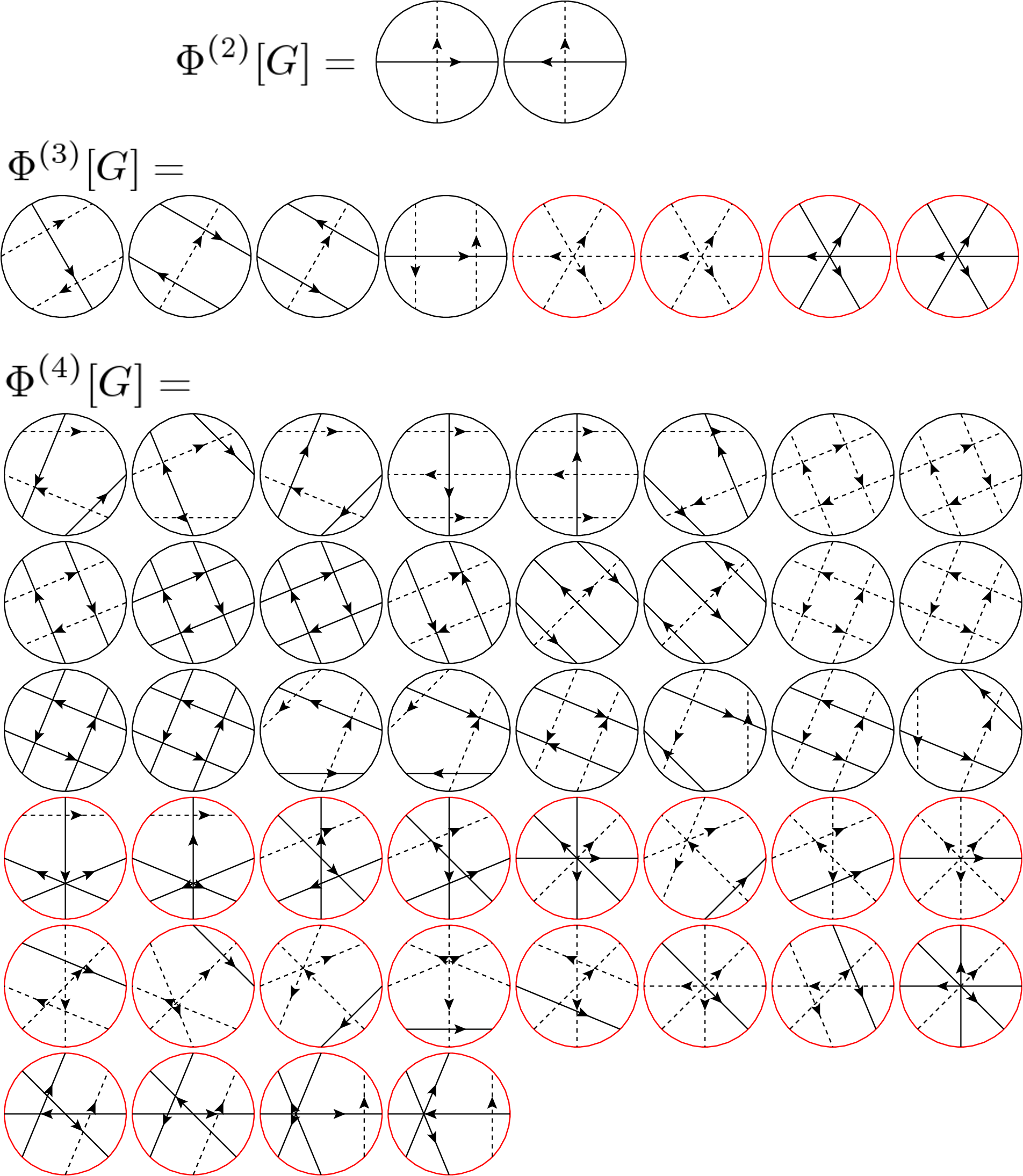
To test the above described algorithm, and to check its performance and convergence, we implemented a simplified version of the bold-ctqmc for the canonical Anderson impurity model. We sampled all diagrams up to certain order starting with first order (NCA), second order (OCA) and up to fifth order. The fifth order takes only minutes on a typical personal computer. We first found the topology of all diagrams of certain order, the prefactor and the sign of each diagram. In Fig. 2 we plotted the diagrams for the first few orders (second - , … fouth - ). We colored the diagrams according to their sign, positive with black and negative with red. There are four NCA diagrams, two OCA diagrams, 8 third order diagrams (4 positive and 4 negative), 44 forth order diagrams (24 positive and 20 negative), 320 fifth order diagrams (128 positive and 192 negative). We evaluated exactly the NCA and OCA diagrams, and we used Metropolis algorithm to sample the time arguments for higher order diagrams. The probability for the acceptance of a set of imaginary times was taken to be proportional to the value of the total , hence at fifth order 320 diagrams were evaluated at each Monte Carlo step. While this algorithm can not be used at very high orders in perturbation theory due to exponential growth in the number of diagrams, its advantage is in large improvement of the sign problem. Namely, the diagrams of the same order and the same time arguments tend to cancel at higher orders. Since we evaluate all of them at each Monte Carlo step, the sign problem is almost completely eliminated.
The non-interacting limit is the hardest case for the hybridization expansion algorithm, because the coherence temperature is infinite. Here we present test of the algorithm in the case of half-filled non-interacting Hubbard model on the Bethe lattice within DMFT. We want to emphasize that the algorithm becomes more efficient and faster converging in strongly interacting limit , a case which will be presented elsewhere.
In Fig. 3(a) we show the impurity Green’s function on imaginary axis (at ) when the perturbation theory is truncated at certain order. We also display the exact result by the dashed line. While the NCA curve clearly deviates from the exact result, the higer order approximations are hardly distinguished from the exact curve on this plot. In Fig. 3b we show separately the contributions to the Green’s function from different orders in perturbation theory. As expected the contribution from the lowest two orders is large, while the higher order contributions are smaller. This shows why OCA approximation is so successful in many realistic situations. The fifth order contribution is on average only , and never exceeds .

In Fig. 4 we zoom-in the exponential drop of the Green’s function at short times. We see that the convergence with the perturbation order is very encouraging.

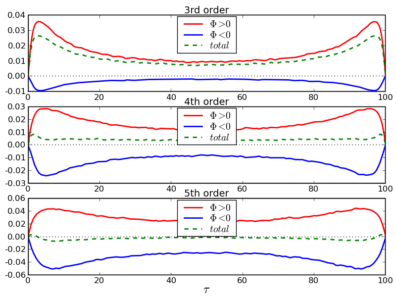
For efficiency of the bold-ctqmc, it is important to monitor the sign of each individual diagram. In Fig. 5 we show separately the contribution to the impurity Green’s function from the diagrams with positive and those with negative , together with the sum of the two. At the third order, the sum is around 70% of the positive contribution, while at the forth and fifth order, the sign drops to 0.2 and 0.07, respectively. As explained above, the current implementation of the method, which groups together all diagrams of a certain order in perturbation theory, does not have a substantial minus sign problem. However, this method becomes expensive at high orders, and thus one needs to resort to sampling of individual diagrams, which can be performed to arbitrary high order. In the latter case, there will be a minus sign problem, as estimated here.
VII.2 The One crossing approximation
In this section we will give the most general formulas for the One crossing approximation, and we will explain the crucial steps in implementing the algorithm.
We start with lowest order approximation, which is the Non-crossing approximation. When evaluating these diagrams, we have to consider only two Hilbert subspaces of constant at once, i.e., and . The first step is to compute all eigenvalues and eigenvectors of the atom in the subspace and . We then group together the atomic eigenstates, which are degenerate, i.e., have the same atomic energy . In the next step we check which of these degeneracy’s survive in the presence of the crystal field environment (impurity hybridization ), and which off-diagonal propagators need to be considered. We evaluate the following matrix elements
| (97) |
Here runs in the Hilbert subspace of and in the Hilbert supspace of . The matrix elements and where is electron destruction operator. The sum runs only over the states which are degenerate and over one electron states which are also degenerate and for which is nonzero in the considered crystal field symmetry. The resulting matrix elements have the same symmetry as the propagators of the pseudoparticles . Clearly, in high symmetry crystal environment, most of the off-diagional matrix elements vanish and the degeneracy of is high, but in low symmetry environment and in the broken symmetry state, many of the off-diagonal propagators become crucial.

Once the symmtry of the propagators is known, we determine all nonvanishing bubbles (NCA diagrams) and the matrix elements for each bubble. The NCA matrix elements are
| (98) |
where we sum only over degenerate states and degenerate crystal field components . The Luttinger-Ward functional and the self-energy corrections are depicted in Fig. 6. We associate a factor to each vertex that marks the creation of electron in bath . Accordingly, we add a factor for each vertex of electron anhilation.

In the next step, we precompute the matrix elements of the one-crossing diagrams, which are depicted in Fig. 7. Here we need to select three different Hilbert subspaces: , , and to compute
| (99) |
Here , , run over the states with , and number of particles, respectively. We add only the most important crossing corrections, for which the particle number is in the Hilbert subspace of the ground state of the atom. We also select to be only the ground state multiplet of the atom, or the atomic states with energy very close to the ground state energy. We compute the matrix elements and only once in the DMFT self-consistent loop and we save them into the input file for OCA impurity solver. The matrix elements , do need to be updated in the outer LDA+DMFT charge loop. We typically update them every three to four charge steps, since the relative crystal field splittings usually change very little during LDA+DMFT iterations. The atomic energies change much more (due to the chemical potential shift), and need to be updated at every step.
The NCA diagrams on the real axis can be evaluated with conventional techniques, and after the projection, they take the following form
| (100) |
| (101) |
where . The pseudoparticle propagators and the pseudoparticle self-energies are related by the Dyson equation. The Eq. 67 shows that .
Many of the pseudoparticle propagators and hybridization functions are degenerate, hence in practice we do not need to sum over all possible , and indices, but we rather use the precomputed matrix elements , which make sure that no equivalent diagram (a diagram which has the same frequency dependence) is not computed multiple times.
To take care of the diverging exponential factors, we work with the projected quantities and , as explained above. The pseudoparticles have typically very sharp almost diverging structure near the treshold energy, which is not easy to Fourier transform. Hence we can not use the Fourier transform for convolutions. We rather cast the above equation into the form for matrix multiplication, for which fast linear algebra packages such as BLAS, exist. We use the logarithmic mesh to resolve the fine structure of the pseudoparticle green’s functions.
It is important to realize that the number of baths is quite small (of the order of for correlated orbital of angular momentum ), while the number of atomic states is much bigger. Hence we precompute the integral and the first moment of functions and of for all . Within trapezoid rule, the values and the first moments of these quantities are enough to compute the above convolutions with matrix multiplications on any given mesh.
To see that, lets consider an arbitrary convolution
| (102) |
Here the function is defined on a certain mesh , on which it is well resolved, i.e., . The function is defined on another mesh , i.e., . The convolution can be safely calculated on the union of both mashes . One of the meshes should be shifted for , thus for each outside frequency, a different union of the two meshes should be formed and only then the convolution can be safely evaluated. This is very time consuming and not done in practice.
When a certain function needs to be convolved with many other functions (like in our example above), we use the followin trick. We first precompute the integral and the first moment of the function
| (103) | |||
| (104) |
We then calculate the convolution without building a new inside mesh. Let’s use the mesh which resolves function . Then, in the spirit of trapezoid rule, we can linearly interpolate between the points
| (106) |
This integral can be expressed by the above defined functions. To show that, let us rewrite the convolution and expressed it by the new function which is defined on the same mesh as and with which the covolution is a simple scalar product
| (107) |
Thus is
| (108) | |||
| (109) |
Hence the convolution of with many functions can be computed at once by the following matrix product .
Once the NCA contributions are evaluated, we add the second order diagrams, which correspond to OCA approximation and are depicted in Fig. 7. They take the explicit form
| (110) | |||
| (111) | |||
| (112) | |||||
| (113) | |||||
In practice, we do not sum over all , and indices. As explained above, we precompute the matrix elements for the most important processes. We take only the low lying atomic states into account (only ’s which are part of the ground state multiplet or with energy very close to the ground state). We also take into account the degeneracy of all atomic states and the degeneracy of baths , in order to avoid computing the equivalent diagram mutliple times. Finally, the convolutions for the OCA approximation can also be cast into the form of matrix multiplication, once the first moment and integrals of a few functions are precomputed.
VIII The analytic continuation method
The Monte Carlo impurity solvers are implemented on imaginary axis where the quantity being sampled is real and many times even “sign-free”. The results obtained in this way are exact, except for the statistical noise. However, even a tiny statistical error on imaginary axis precludes the analytic continuation by Pade type of methods. The standard method, to overcome the difficulty of the singularity of the kernel, is the Maximum Entropy Method (MEM). The basic idea of this method is to find a function on the real axis, which is very close to Monte Carlo data on imaginary axis (within statistical error), and is smooth function on real axis, locally not very different from a chosen model function. This approach works very well for analytical continuation of the Green’s function to obtain spectral function on real axis, i.e., to solve the integral equation
for .
Knowing the spectral function, it is however not possible to obtain the momentum resolved spectra, or optical conductivity, or transport coefficients. To compute these properties, it is essential to analytically continue the self-energy, rather then the Green’s function. The self-energy of correlated materials is however very hard to analytically continue with maximum entropy method, because the self-energy typically has very sharp feature or even poles, which separate the low energy part of the spectra (the quasiparticle peak) from the high energy part of the spectra (the Hubbard bands). Due to the maximum entropy method requirements of smoothness, the analytically continued self-energy at low energy is typically polluted with the near-by poles, which appear in the self-energy at the intermediate energy.
A successful analytic continuation method for self-enery needs to met the following conditions:
- •
imaginary axis self-energy is equal to Monte Carlo data within the statistical error
- •
real axis self-energy function must be locally smooth
- •
the power-expansion around zero frequency should match the quantum Monte Carlo data on both, real and imaginar axis.
While the first two conditions are met by MEM, the last is not.
We developed an alternative method, which mets the above conditions and was very successfully used in combination with CTQMC for pnictides [11], cuprates [64], VO2 and other materials. Although the method has many parameters, which needs to be choosen appropriately, we can always check its accuracy by recomputing the spectral function of the lattice, using analytically continued self-energy, and comparing the spectral function to the maximum entropy continued spectra.
We expand the self-energy in terms of modified Gaussians , and we add a polynomial function around zero frequency
| (114) |
The modified Gaussians
| (115) |
have a unique peoperty that they are peaked at , with the width of approximately , while they exponentially vanish at zero frequency. They are asymmetric with slow decay away from zero and very fast decay towards zero frequency. We choose the modified Gaussians centered on a logarithmic mesh of with . The modified Gaussians functions were used in connection with constructing the NRG spectral function [65]. We typically take the parameter to be .
Since the modified Gaussians all vanish at zero frequency, we add a polynomial function around zero frequency. The coefficients of the polinomial are determined by fitting the imaginary axis self-energy, i.e.,
| (116) |
which can be analytically continued to
| (117) |
The polynomial has to drop-off sufficiently fast at high frequency, hence we choose the following function
| (118) |
where the upper choice is made for metals and the lower choice for insulators and very bad metals. In the FL regime, we have , . The coefficient is determined by the condition
For speed, we precompute and by
| (119) |
Similarly, we also precompute and . Also the integral of the functions and are precomputed.
The coefficients in expansion Eq. (114) are determined by minimizing the following functional
| (120) | |||
| (121) |
Here in the first term runs over the imaginary frequencies which are sampled by QMC (and not over the analytically added tail). The second terms imposes the correct value of the integral of the self-energy. The integral of the expansion (114) is
which needs to match the tail of the QMC data
Finally, the last three terms ensure that the value, and the first two derivatives of the analytically continued self-energy at zero frequency match the derivatives on imaginary axis. For minimization, we use the L-BFGS-B alrorithm of Ref. 66.
IX Cerium - transition

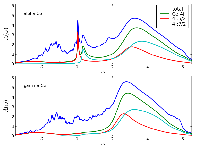


To test our implementation of DFT+DMFT within Wien2K method, we show in Figs. 8 and 9 results for cerium to transition.
At a temperature less than K and pressure less than 20 kbar, elemental cerium undergoes a transition between two isostructural phases: a high pressure phase or phase and a low pressure phase. In -Ce the electron is delocalized while in -Ce the electron is localized. The transition is well accounted for by phenomenological Kondo Volume Collapse picture [68, 69, 70].
We treat only the Ce electrons as strongly correlated thus requiring full energy resolution, while all other electrons such as Ce are assumed to be well described by the GGA. We choose eV and eV for the Coulomb interaction. The value of was obtained by constraint DFT calculation [71] and was computed using the atomic physics program of Ref. 42 and reduced by 30% to account for the screening in the solid. Both phases of Ce have fcc unit cell with quite different volumes, and . The results were converged with 5000- points, we use the GGA functional for the DFT part and use OCA and CTQMC impurity solver to solve the auxliliary impurity problem.
The results in Fig. 8 (obtained by OCA) and Fig. 9 (obtained by CTQMC) are practically identical and very similar to previous LDA(LMTO)+DMFT results [72]. One can clearly see the broad quasiparticle peak in -Ce, split by the spin-orbit coupling eV. The lower peak has mostly character and the upper peak mostly -character. The system is in good Fermi liquid regime at the temperature of K used in the calculation. The second phase with larger volume is in local moment regime with no visible Kondo peak at the Fermi level, but enhanced Hubbard bands.
It is instructive to examine the hybridization function as computed by LDA and self-consistent DMFT (see Fig. 10). It turns out that in Ce, the low energy hybridization function is substantially reduced compared to its LDA value. The two large peaks at eV and eV are absent in DMFT hybridization. Since the coherence scale is exponential function of hybridization, the coherence scale is lower in DMFT than it would be in so called one-shot DMFT. It is known from the early days of the Kondo volume collapse theory [69], that the LDA hybridization in a one-shot calculation was too big and had to be renormalized by phenomenological parameter [73]. DMFT reduces the hybridization through the collective screening effects and hence is able to give correct coherence scale of the problem.
Finally, let us show optical conductivity, as implemented in LDA(Wien2K)+DMFT method. The overal agrement with previous LDA+DMFT results [10] is very good. The new computational results are in even slightly better agreement with experiment of Ref. 67, since they both clearly display a shoulder around eV in -Ce, which we can now clearly identify as excitations across the split quasiparticle peak. The splitting is due to spin-orbit coupling in Ce.
X Heavy fermion 115 materials
The heavy fermion 115 materials have a chemical formula CeIn5, where is either Co, Rh or Ir. They crystallize in layered tetragonal structure shown in Fig. 12, composed of Ce-In layers and -In layers.
At high temperature, the low energy electronic states are composed of mainly the broad bands of In and Ce. The Ce- electrons are localized and their spectra is mostly contained in Hubbard bands, which are more than eV away from the Fermi level. These electrons behave as local magnetic moments. As the temperature is reduced, the moments combine with the conduction electrons to form a fluid of very heavy quasiparticles, with masses that are two or three orders of magnitude larger then the mass of the electrons.

The low temperature physics of 115 materials is very puzzling. The heavy fermion physics comes primarily from the Ce-In layer. Indeed, the related material CeIn3 has only the Ce-In layers (no -In layer), and also displays a similar heavy fermion properties with superconductivity at very low temperature. However, 115 materials are very sensitive to the substitution of the transition metal ion in the -In layer although Co, Rh and Ir ions have the same valence (they are isovalent). Indeed the three 115 materials have dramatically different low energy properties: CeCoIn5 is a superconductor with K, CeRhIn5 is antiferromagnet with K, while CeIrIn5 is superconductor with of only K. A fundamental question arises: Why are the low energy properties of 115 materials so different?
A hint to the resolution of this problem was given in Ref. 58, where the DFT+DMFT calculation for CeIrIn5 indicated that the Ce electrons hybridize stronger to the out of plane In- electrons, than the in-plane In electrons. Here we carried out the DFT+DMFT calculation for all three 115 materials and we show the difference in electronic structure between the three materials. We used the code based on LDA-LMTO code of Ref. 32 as well as the new LAPW code based on Wien2K [31] code. The results obtained by our DFT+DMFT method in the two codes are almost indistinguishable. For the impurity solver, we used both OCA (described above) and CTQMC [23]. The analytic continuation of CTQMC results was performed with the method described in chapter VIII.


Fig. 13A shows the total density of states (DOS) and the partial Ce- DOS for all three materials at low temperature of 7 K. The transition metal ion DOS is peaked around binding energy 2eV, where the difference of DOS is large. The partial Ce- DOS of the three compound is very similar, except at the very low energy. Fig. 13B zooms-in the low energy part of the spectra. We see that CeIrIn5 compound has the largest quasiparticle peak, the CeCoIn5 follows, while the CeRhIn5 has substantially smaller quasiparticle peak at the same temperature of K.

Our view on the localization-itinerancy in 115 materials is sketched in Fig. 14. Rh compound is most localized, while Ir compound is most itinerant. Co compound is similar to Ir compound, but slightly less itinerant than Ir-115.
It is well known from the pressure experiments [74, 75] that Rh compound is more localized then Co compound. Namely, under pressure of 1 GPa the Rh compound becomes superconducting, and at pressure of GPa reaches similar maximum TC as is the maximum TC of Co compound [76]. Hence the pressure of the order of GPa sufficiently increases the Ce- hybridization that it overcome the difference between localization of the electrons in the two compounds. Experimentally it is a bit less clear what is the relation between Ir and Co compound, since both compounds are superconductors at low T. Ir compound has somewhat smaller specific heat coefficient in normal state than Co compound ( mJ/ for Ir-115 versus 1000 mJ/ for Co-115) [77, 78]. Ir compound has also somewhat lower resistivity in the normal state [79]. Moreover, nuclear quadrupol resonance (NQR) measurements of [80] suggest that Ir-compound might be more itinerant than other Ce-compound. Indeed pressurizing the CeIrIn5 [81] along the crystallographic -direction, which increases itinerancy [82], decreases TC. Furthermore, it was shown that Cd-doping acts as reverse pressure in 115’s [83]. Since higher Cd-doping is necessary for appearance of antiferromagnetic phase in CeIrIn5 than in CeCoIn5, this is also suggestive of more itinerant nature of Ir-compound.
Our results are thus consistent with the resistivity experiments [79], NQR experiments [80] and recent pressure experiments [81], and indicate that Ir compound is on the itinerant side of the phase diagram. Hence the low superconducting transition temperature might be connected with too itinerant nature of carriers.


We further analize the difference in itinerancy by plotting the hybridization function at zero frequency resolved in crystal field basis. The dimensional matrix of hybridizations has a 6 dimensional component and a 9 dimensional component. The itinerancy (the quasiparticle peak) is almost entirely from the component, hence we will not analize part. The degeneracy of the shell is lifted in tetragonal crystal environment and hybridization splits into , and components. The corresponds to , while and correspond approximately to and , respectively. In Fig. 15 we plot the hybridization () in polar coordinates with Ce atom in the center and In atoms around. The plot is the cut in direction. The three dimensional orbitals that correspond to the three crystal fields are plotted in the lower pannel of Fig. 15 together with the real space positions of In and Ce atoms. In this decomposition, hybridizations and are pointing towards out of plane In (In2) and in-plane In (In1), respectively. The third component, is pointing towards transition metal ion.
When comparing hybridization of the three 115 compounds, the Ir compound has all three components of the hybridization larger than the other two compounds. In Co-115 all three hybridizations are slightly smaller, while in Rh-115 all three hybridizations are substantially smaller.
Furthermore, comparing the strength of the three components of the hybridization, one can notice that in Ir compound the component, pointing towards out-of plane In, is largest. This is consistent with the experimental finding of Oeschler et al. [82] that the Grüneisen parameters in -direction is 2.5 times bigger that in direction, resulting in larger effective coherence scale in -direction.
In Co-compund the and components have similar strength, while is smaller, hence the hybridization in -direction is still more important than in -plane, consistent with Grüneisen parameter measurements [82]. It was shown in Ref. 58 that the double peak structure of the optical conductivity is directly related to the strength of the two hybridizations. The hybridization gap in one part of the momentum space is larger, and is primarily due to out of plane In, and the hybridization gap in some other part of momentum space, controled mainly by the in-plane In, is smaller, resulting in double peak structure of the mid-infrared optics peak. Optical measurements on CeCoIn5 of Singley et al[84] demonstrated very clearly that the mid-infrared peak is split into two peaks, one at cm-1 and one at cm-1, which can hint towards substantial difference in the two types of hybridization.
Finally, in contrast to Ir and Co compound, Rh compound has largest hybridization, followed by and .

In Fig. 16 we show the frequency dependent hybridization function to demonstrate that the retardation effects in heavy fermion materials are very nontrivial and that the buildup of the quasiparticle peak in spectral function usually results in a sharp peak in hybridization, on the background of the depleted region of hybridization. The peak is sometimes called the collective hybridization, because it arises from the lattice effects. Namely, the Ce- electrons on neighboring atoms also become delocalized, enhancing the hybridization at low energy. However, the spd-electrons need to screen many Ce- moments, and therefore the effective hybridization is actually slightly reduced, resulting in depletion away from the Fermi level, sometimes called Kondo hole.
Our results demonstrate that the degree of itinerancy is controlled by the collective hybridization, encoded into the Weiss mean field hybridization within DMFT. But what is the origin of the difference between the three compounds? In Fig. 14 we show the parameters of the lattice structure, namely the Ce-In(1) distance, the Ce-In(2) distance and the angle between the CeIn3 plane and out of plane In (In2). From these numbers, it is clear that none of the three quantities follows the trend of itinerancy. Hence the difference in the lattice structure is likely not the key element.
To demonstrate that the difference in the lattice structure is not the driving force, we performed the DMFT calculation for the three compounds using the same lattice structure of CeIrIn5. The results were very similar to the results plotted in Fig. 13, with only slight increase in itinerancy of Rh compound. This demonstrates that the chemistry of the transition metal ion (difference between , and orbitals) is the driving force of the itinerancy, and not the diffrence in the crystal structure. The latter are the secondary effects.

Since CeRhIn5 remains in local moment regime down to very low tempeture of the order of the RKKY interaction, it is worth trying to stabilize a magnetic solution within DMFT. To this end, we doubled the unit cell and allowed the comensurate antiferromagnetic ordering with the wave vector . Experimentally, the order is a helical spiral with wave vector and of K. The broken symmetry solution can be stabilized below K as shown in Fig. 17. The magnetization has a typical mean field form, as expected for a theory with spatial mean-field character like DMFT.


An interesting question is how does the large moment antiferromagnetic solution change the emerging quasiparticle peak. We have shown in Fig. 13 that even in more localized CeRhIn5 a peak starts to develop at the Fermi level by decreasing temperature, hence coherence starts to develop at quite high temperature similar to the other two compounds. However, the height of the quasiparticle peak is smaller and the scattering rate of Ce- orbital (imaginary part of the self-energy) is higher in CeRhIn5. The long range order state develops from a state with a partially screened moment. In Fig. 18 we show the density of states of the two phases, the paramagnetic state and the Neel state. The latter has no quasiparticle peak left and only a very broad background of the spectral weigh remains at the Fermi level. The lower panel of Fig. 18 compares a very coherent quasiparticle peak of CeIrIn5 with the partially screened state of CeRhIn5 above and in the ordered state below , to emphasize the dramatic difference in the density of state at low energy. Because the full coherence of quasiparticles is not reached to very low temperature in CeRhIn5, and the non-local RKKY interaction is strong enough, it interrupts the formation of coherent quasiparticles. Within DMFT, this is reflected in two stable solutions of DMFT equations, the paramagnetic and the magnetic solution. We note that we did not prove the stability of the magnetic solution compared to the paramagnetic solution, because this would require a comparison between free energies, a task beyond our current capabilities. However, our experience from model calculations suggests that when the magnetic DMFT solution can be stabilized, it usually has lower free energy than the nonmagnetic solution.
XI Conclusion
In the first part of the article, we discussed in detail the implementation of DFT+DMFT in full potential methods. We defined the central object of the DMFT, the local Green’s function using a projection operator. We showed that the projector used in LDA+U implementations leads to non-causal DMFT equations and that the straightforward projection to the solution of the Schrödinger equation within the Muffin Tin sphere leads to spectral weight loss. We suggested an alternative projection that resolves these shortcomings.
We sketched the algorithmic steps within an implemention of DFT+DMFT in the full potential methods, using a formulation which avoids the ambiguities of downfolding or Wannier orbital construction. Hence, the kinetic energy operator and electron density are not approximated by a tight-binding parameterization, which allowed us to carry out a charge density self-consistent calculation.
In the second part of the article, we concentrated on impurity solvers based on the hybridization expansion. We derived the equations for the bold continuous time quantum Monte Carlo (CTQMC) method, which samples the dressed propagators, as opposed the bare propagators sampled in current CTQMC methods. We showed a few test results for simplified implementation of the method. In this part of the article we also gave detailed formulas for the impurity solver called the One-crossing approximation, which can be viewed as the four kink approximation within the bold CTQMC.
Finally we give details on a new analytic continuation method, which can continue the self-energy from the imaginary to the real axis. This step is crucial when computing the response functions within DMFT, as done in section VI for transport coefficients.
In the third part of the article, we presented the test results of our DFT+DMFT implementation on a classical problem of strong correlations, the isostructural transition of elemental cerium from its phase at high temperature to its phase at low temperature.
In the last part of the article, we applied the DFT+DMFT method to a group of heavy fermion compounds, namely CeIrIn5, CeCoIn5 and CeRhIn5, collectively dubbed the Ce-115s. Although the isovalent substitution of a transition metal ion does not substantially alter the Ce-In planes, which are believed to be responsible for the heavy mass in these compounds, the ground state properties of these materials are very different.
We analyzed the electronic structure of the three Ce-115 materials and showed that the Ce- electrons in CeRhIn5 are more localized that those in the other two 115 compounds, in agreement with experiments. Below K, an antiferromagnetic DFT+DMFT solution in CeRhIn5 is stable, while CeCoIn5 and CeIrIn5 remain paramagnetic (the AFM solution is not stable) down to the lowest temperature K explored in our calculation.
The hybridization in CeIrIn5 is very anisotropic with the largest component pointing towards the out-of-plane In. The hybridization is slightly smaller in CeCoIn5, hence we believe CeIrIn5 to be more itinerant than the other two compounds.
We speculate that the reason CeCoIn5 exhibits the highest superconducting TC is due to the fact that it is at the border between itinerancy and localization, while CeIrIn5 is on the itinerant side of the phase diagram and CeRhIn5 is on the localized side. The position of CeRhIn5 in the phase diagram is clear from the pressure experiments, while the position of CeIrIn5 is less obvious. We believe that recent uniaxial pressure experiments [81] confirm our view, since the -axis compression, which makes CeIrIn5 more itinerant, decreases the superconducting .
XII Acknowledgement
We thank Gabriel Kotliar for careful reading of the manuscript and numerous usefull suggestions from the early stage of the project till its completion. We are grateful to Jim Allen and David Pines for fruitful discussion. K.H was supported by Grant NSF NFS DMR-0746395 and DMR-0806937, and Alfred P. Sloan fellowship. C.H.Y was funded by NSF DMR-0806937 and K.K. by Petroleium Research Fund 48802-DNI10.
Note added: As the writing of this work was being completed, we became aware of a related work of M. Aichhorn et al. (arXiv: 0906.3735) also reporting on an implementation of LDA+DMFT in a LAPW code. However, in contrast to our implementation, the authors used downfolding method to obtain a tight-binding model Hamiltonian, and hence could not compute electronic charge self-consistently. In the process of downfolding, the authors used projection defined in section II. Furthermore, the impurity solver did not take into account the full Coulomb interaction Eq. (28). Only the density-density part of the interaction was considered by M. Aichhorn et al. (only the component of the Hund’s coupling) which allows substantial simplification of the impurity solver, but leads to improper description of the multiplet structure of the correlated atoms.
Appendix A Complex Tetrahdron Method
The formulas for tetrahedron integral in case of complex eigenvalues are very similar to the case of real eigenvalues. However, a special attention needs to be payed to choose the right branch-cut in logarithms, such that all terms in the sum are causal.
First step in tetrahedron method consists of dividing the first Brillouin zone into tetrahedra which fill up whole space. Each thrahedra has four corners. The energy is thus interpolated , where , and run between 0 and 1 when visiting corners of tetrahedra.
For the Green’s function we need integral of the form
| (122) |
and for the electron density and the chemical potential we need
| (123) |
The integral is first written as the sum over all tetrahedra and the integral in the interior of tetrahedra:
| (124) |
The latter is evaluated analytically using linear interpolation inside the volume of the tetrahedra for both the nominator and denominator
| (125) | |||
Here we used a short notation
The integrals are analytic and a closed expression for computing the green’s function is
where
| (126) |
and means and . Notice that only and can appear in (not ) to ensure causality. Namely, imaginary part of all is strictly negative, hence the expression contains and , which both have imaginary part in the interval .
Similarly, the formulas for the integral over frequency are
| (127) | |||||
where
| (128) | |||||
and
Appendix B Transport integrals
To compute the transport coefficients, we need to evaluate to high precision the following integrals
| (129) | |||||
| (130) | |||||
| (131) |
The integrals need to be carefully implemented and special care needs to be taken for the two case: a) and b) and .
The first integral of Eq. (129) is computed numerically, except in the following cases
where
is precomputed on a fine mesh and interpolated using cubic spline interpolation. The constants are
| (135) |
The second integral of Eq. (130) is computed numerically, except in the following cases i) : In this limit it becomes , ii) : In this case, the power expansion in terms of is performed and all terms are analytically evaluated.
Similarly we treat integral Eq. (131). For , we approximate and for we perform the power expansion in terms of and analytically evaluated the resulting integrals.
References
- [1] A. Georges, G. Kotliar, W. Krauth, and M. J. Rozenberg, Rev. Mod. Phys. 68, 13 (1996).
- [2] V. I. Anisimov, A. I. Poteryaev, M. A. Korotin, A. O. Anokhin, and G. Kotliar, J. Phys. Cond. Matter 9, 7359 (1997).
- [3] A. I. Lichtenstein and M. I. Katsnelson, Phys. Rev. B 57, 6884 (1998).
- [4] Gabriel Kotliar and Dieter Vollhardt, Physics Today 57, 53 (2004).
- [5] G. Kotliar, S. Y. Savrasov, K. Haule, V. S. Oudovenko, O. Parcollet, and C. A. Marianetti Rev. Mod. Phys. 78, 865 (2006).
- [6] S. Y. Savrasov, G. Kotliar, and E. Abrahams, Nature London, 410, 793 (2001).
- [7] S. Y. Savrasov, K. Haule, and G. Kotliar, Phys. Rev. Lett. 96, 036404 (2006).
- [8] J. H. Shim, K. Haule, S. Savrasov, G. Kotliar, Phys. Rev. Lett. 101, 126403 (2008).
- [9] X. Dai, S. Y. Savrasov, G. Kotliar, A. Migliori, H. Ledbetter, and E. Abrahams, Science 300, 953 (2003).
- [10] K. Haule, V. Oudovenko, S. Y. Savrasov, and G. Kotliar, Phys. Rev. Lett. 94, 036401 (2005).
- [11] K. Haule, J. H. Shim, G. Kotliar, Phys. Rev. Lett. 100, 226402 (2008).
- [12] J. H. Shim, K. Haule, and G. Kotliar, Nature London 446, 513 (2007).
- [13] C. A. Marianetti, K. Haule, G. Kotliar, and M. J. Fluss, Phys. Rev. Lett. 101, 056403 (2008).
- [14] J. H. Shim, K. Haule, G. Kotliar, Eur. Phys. Lett. 85, 17007, (2009).
- [15] V. S. Oudovenko, G. Palsson, K. Haule, G. Kotliar, and S. Y. Savrasov, Phys. Rev. B 73, 035120 (2006).
- [16] S.Y. Savrasov, and G. Kotliar, Phys. Rev. B 69, 245101 (2004).
- [17] Alexander B. Shick, Jindrich Kolorenc, Alexander I. Lichtenstein, Ladislav Havela, arXiv:0903.1998.
- [18] J. Minar, L. Chioncel, A. Perlov, H. Ebert, M. I. Katsnelson, and A.I. Lichtenstein, Phys. Rev. B 72, 045125 (2005).
- [19] F. Lechermann, A. Georges, A. Poteryaev, S. Biermann, M. Posternak, A. Yamasaki, and O. K. Andersen, Phys. Rev. B 74, 125120 (2006).
- [20] B. Amadon, F. Lechermann, A. Georges, F. Jollet, T. O. Wehling, and A. I. Lichtenstein, Physical Review B 77, 205112 (2008).
- [21] P. Werner, A. Comanac, L. de Medici, M. Troyer, and A. J. Millis, Phys. Rev. Lett. 97, 076405 2006.
- [22] A. N. Rubtsov, V. V. Savkin, and A. I. Lichtenstein, Phys. Rev. B 72, 035122 2005.
- [23] Kristjan Haule, Phys. Rev. B 75, 155113 (2007).
- [24] P. Werner and A.J. Millis, Phys. Rev. B 74, 155107 (2006).
- [25] K. Haule, S. Kirchner, J. Kroha, and P. Wölfle, Phys. Rev. B 64, 155111 (2001).
- [26] X. Dai, K. Haule, and G. Kotliar, Phys. Rev. B 72, 045111 (2005).
- [27] S. Y. Savrasov, V. Oudovenko, K. Haule, D. Villani, and G. Kotliar, Phys. Rev. B 71, 115117 (2005).
- [28] V. I. Anisimov et. al, Phys. Rev. B 71, 125119 (2005).
- [29] H. Hafermann, C. Jung, S. Brener, M. I. Katsnelson, A. N. Rubtsov, A. I. Lichtenstein, Europhys. Lett. 85, 27007 (2009).
- [30] D. J. Singh, L. Nordstrom, Planewaves, Pseudopotentials, and the LAPW Method, (Springer, New York, 2006).
- [31] P. Blaha, K. Schwarz, G. K. H. Madsen, K. Kvasnicka, and J. Luitz, Wien2K (Karlheinz Schwarz, Technische Universitat Wien, Austria, 2001).
- [32] S.Y. Savrasov, Phys. Rev. B 54, 16470 (1996).
- [33] K. Held et al., Psi-k Newsletter #56 (April 2003), p. 65;
- [34] A. I. Lichtenstein, M. I. Katsnelson, and G. Kotliar,in Electron Correlations and Materials Properties 2, ed. A. Gonis (Kluwer, NY)[cond-mat/0211076].
- [35] E. Pavarini, S. Biermann, A. Poteryaev, A. I. Lichtenstein, A. Georges, and O. K. Andersen, Phys. Rev. Lett. 92, 176403 (2004).
- [36] L.V. Pourovskii, B. Amadon, S. Biermann, A. Georges, Phys. Rev. B 76, 235101 (2007).
- [37] Dm. Korotin, A. V. Kozhevnikov, S. L. Skornyakov, I. Leonov, N. Binggeli, V. I. Anisimov, G. Trimarchi, The European Physical Journal B 65, 1, 91-98 (2008).
- [38] N. Marzari and D. Vanderbilt, Phys. Rev. B 56, 12847 (1997).
- [39] P. Novak, Program QTL - technical report, part of the Wien2K-code documentation.
- [40] A.B. Shick, A.I. Liechtenstein, W.E. Pickett, Phys. Rev. B 60, 10763 (1999).
- [41] F. Aryasetiawan, K. Karlsson, O. Jepsen, U. Schonberger, Phys. Rev. B 74, 125106 (2006).
- [42] R. D. Cowan, The Theory of Atomic Structure and Spectra (Univ. California Press, Berkeley, 1981).
- [43] L.D. Marks, and D.R. Luke, Phys. Rev. B 78, 075114 (2008).
- [44] Ph. Lambin and J. P. Vigneron, Phys. Rev. B 29, 3430 (1984).
- [45] A. Khurana, Phys. Rev. Lett. 64 1990.
- [46] K. Haule, and G. Kotliar, arXiv:0907.0192.
- [47] H. Keiter and J.C. Kimball, Int. J. Magn. 1, 233, (1971).
- [48] N. Grewe and H. Keiter, Phys. Rev. B 24, 4420 (1981).
- [49] Y. Kuramoto, Z. Phys. B 53, 37 (1983).
- [50] N. Grewe, Z. Phys. B 53, 271 (1983).
- [51] H. Keiter and G. Morandi, Phys. Rep. 109, 227 (1984).
- [52] P. Coleman, Phys. Rev. B 29, 3035 (1984).
- [53] N. E. Bickers, Rev. Mod. Phys. 59, 845 (1987).
- [54] Th. Pruschke and N. Grewe, Z. Phys. B: Condens. Matter 74, 439 (1989).
- [55] J. Kroha, P. Wölfle, and T. A. Costi, Phys. Rev. Lett. 79, 261 (1997).
- [56] N. Grewe, S. Schmitt, T. Jabben, F.B. Anders, J. Phys.: Condens Matter 20, 365217 (2008).
- [57] J. H. Shim, K. Haule, and G. Kotliar, Nature 446, 513 (2007).
- [58] J.H. Shim, K. Haule and G. Kotliar, Science 318, 1615 (2007).
- [59] C. A. Marianetti, K. Haule, G. Kotliar, and M.J. Fluss, Phys. Rev. Lett. 101, 056403 (2008).
- [60] E. Gull, P. Werner, A. Millis, and M. Troyer, Phys. Rev. B 76, 235123 (2007).
- [61] N. Prokof’ev, B. Svistunov, Phys. Rev. Lett 99, 250201 (2007).
- [62] J. Kroha and P. Wölfle, Acta Phys. Pol. B 29, 3781 (1998).
- [63] E. Kozik, K. Van Houcke, E. Gull, L. Pollet, N. Prokof’ev, B. Svistunov, M. Troyer, arXiv:0907.0863v1.
- [64] Cedric Weber, Kristjan Haule, Gabriel Kotliar, Phys. Rev. B 78, 134519 (2008).
- [65] Ralf Bulla, Theo Costi, Thomas Pruschke, Rev. Mod. Phys. 80, 395 (2008).
- [66] R. H. Byrd, P. Lu and J. Nocedal, SIAM Journal on Scientific and Statistical Computing, 16, 1190, (1995).
- [67] J. W. van der Eb, A. B. Kuz’menko, and D. van der Marel, Phys. Rev. Lett. 86, 3407 (2001).
- [68] J. W. Allen, S. J. Oh, M. B. Maple and M. S. Torikachvili,Phys. Rev. B 28, 5347 (1983).
- [69] J. W. Allen and Richard M. Martin, Phys. Rev. Lett. 49, 1106 (1982).
- [70] J. W. Allen, J. Phys. Soc. Japan 74, 34 (2005).
- [71] A. K. McMahan, C. Huscroft, R. T. Scalettar, and E. L. Pollock, J. Comput,-Aided Mater. Des. 5, 131 (1998).
- [72]
DFT(LMTO)+DMFT results for various correlated
materials are collected in a database available at
ttp://auleweb.rutgers.edu/database/ .The DFT(LMTO)+DMFT code is available for download at the same adress. The DFT(Wien2K)+DMFT will be posted at the same address. - [73] J. W. Allen, private communication.
- [74] H. Hegger, C. Petrovic, E. G. Moshopoulou, M. F. Hundley, J. L. Sarrao, Z. Fisk, and J. D. Thompson, Phys. Rev. Lett. 84, 4986 (2000).
- [75] A. Llobet, J. S. Gardner, E. G. Moshopoulou, J.-M. Mignot, M. Nicklas, W. Bao, N. O. Moreno, P. G. Pagliuso, I. N. Goncharenko, J. L. Sarrao, and J. D. Thompson, Phys. Rev. B 69, 024403 (2004).
- [76] T. Park, F. Ronning, H. Q. Yuan, M. B. Salamon, R. Movshovich, J. L. Sarrao and J. D. Thompson, Nature 440, 65 (2006)
- [77] C. Petrovic, R. Movshovich, M. Jaime, P. G. Pagliuso, M. F. Hundley, J. L. Sarrao, Z. Fisk, and J. D. Thompson, Europhys. Lett. 53 354, (2001).
- [78] R. Movshovich, M. Jaime, J. D. Thompson, C. Petrovic, Z. Fisk, P. G. Pagliuso , and J. L. Sarrao, Phys. Rev. Lett. 86, 5152 (2001).
- [79] H. Shishido, R. Settai, D. Aoli, S. Ikeda, H. Nakawaki, N. Nakamura, T. Iizuka, Y. Inada, K. Sugiyama, T. Takeuchi, K. Kindo, T. C. Kobayashi, Y. Haga, H. Harima, Y. Aoki, T. Namiki, H. Sato, and Y. Nuki, J. Phys. Soc. Jpn, 71, 162 (2002).
- [80] G.-q. Zheng, K. Tanabe, T. Mito, S. Kawasaki, Y. Kitaoka, D. Aoki, Y. Haga, and Y. Onuki, Phys. Rev. Lett. 86, 4664 (2001).
- [81] O. M. Dix, A. G. Swartz, and R. J. Zieve, J. Cooley, T. R. Sayles and M. B. Maple Phys. Rev. Lett. 102, 197001 (2009).
- [82] N. Oeschler, P. Gegenwart, M. Lang, R. Movshovich, J. L. Sarrao, J. D. Thompson, and F. Steglich, Phys. Rev. Lett. 91, 076402 (2003).
- [83] L. D. Pham, T. Park, S. Maquilon, J. D. Thompson, and Z. Fisk, Phys. Rev. Lett. 97, 056404 (2006).
- [84] E. J. Singley, D. N. Basov, E. D. Bauer, and M. B. Maple, Phys. Rev. B 65, 161101(R) (2002).