A refinement of the Conway-Gordon theoremsThanks: The author was partially supported by Grant-in-Aid for Young Scientists (B) (No. 21740046), Japan Society for the Promotion of Science.

Throughout this paper we work in the piecewise linear category. Let $f$ be an embedding of a finite graph $G$ into ${\mathbb{R}}^{3}$. Then $f$ (or $f(G)$) is called a spatial embedding of $G$ or simply a spatial graph. Two spatial embeddings $f$ and $g$ of $G$ are said to be ambient isotopic if there exists an orientation-preserving self homeomorphism $\Phi$ on ${\mathbb{R}}^{3}$ such that $\Phi\circ f=g$. We call a subgraph $\gamma$ of $G$ which is homeomorphic to the circle a cycle of $G$, and a cycle of $G$ which contains exactly $k$ edges a $k$-cycle of $G$. We denote the set of all cycles of $G$, the set of all $k$-cycles of $G$ and the set of all pairs of two disjoint cycles consisting of a $k$-cycle and an $l$-cycle of $G$ by $\Gamma(G)$, $\Gamma_{k}(G)$ and $\Gamma_{k,l}(G)$, respectively. For $\gamma\in\Gamma(G)$ (resp. $\lambda\in\Gamma_{k,l}(G)$) and a spatial embedding $f$ of $G$, $f(\gamma)$ (resp. $f(\lambda)$) is none other than a knot (resp. $2$-component link) in $f(G)$.

Let $K_{n}$ be the complete graph on $n$ vertices, namely the graph consisting of $n$ vertices $1,2,\ldots,n$, a pair of whose vertices $i$ and $j$ is connected by exactly one edge $\overline{ij}$ if $i\neq j$. Let us recall the following two famous theorems in spatial graph theory, which are called the Conway-Gordon theorems.

Conway-Gordon’s formulas (1.1) and (1.2) hold only modulo two. Note that the square of the linking number is congruent to the linking number modulo two, and the second coefficient of the Conway polynomial of a knot is congruent to the Arf invariant modulo two [7]. Our first purpose in this article is to refine Conway-Gordon’s formulas above by giving their integral lifts in terms of the square of the linking number and the second coefficient of the Conway polynomial as follows.

Note that Theorems 1-1 and 1-2 can be obtained from Theorems 1-3 and 1-4 respectively by taking the modulo two reduction. We also show that Theorem 1-4 can be divided into the following two formulas.

Note that Theorem 1-4 can be recovered from (1.3) and (1.4). We give proofs of Theorems 1-3, 1-4 and Corollary 1-5 in section $3$. We remark here that the second coefficient of the Conway polynomial and the square of the linking number are Vassiliev invariants [21] of order $2$ [2], [10]. See also [14] for general results about Vassiliev invariants of knots and links in a spatial graph.

Our second purpose in this article is to give applications of Theorems 1-3 and 1-4 to the theory of rectilinear spatial graphs. Here a spatial embedding $f$ of a graph $G$ is said to be rectilinear if for any edge $e$ of $G$, $f(e)$ is a straight line segment in ${\mathbb{R}}^{3}$. Note that for any positive integer $n$, there exists a rectilinear spatial embedding of $K_{n}$. Actually it can be constructed by taking $n$ vertices on the moment curve $(t,t^{2},t^{3})$ in ${\mathbb{R}}^{3}$ and connecting every pair of two distinct vertices by a straight line segment (this also implies that any simple graph has a rectilinear spatial embedding). Note that every knot or link contained in a rectilinear embedding of $K_{n}$ has stick number less than or equal to $n$, where the stick number $s(L)$ of a link (or a knot) $L$ is the minimum number of edges in a polygon which represents $L$. The following are fundamental results on stick numbers for knots and $2$-component links, see [11], [1], [8].

Therefore we have that non-trivial knots in a rectilinear spatial embedding of $K_{6}$ (resp. $K_{7}$) are only trefoil knots (resp. trefoil knots and figure eight knots), and non-trivial $2$-component links in a rectilinear spatial embedding of $K_{6}$ (resp. $K_{7}$) are only Hopf links (resp. Hopf links and $(2,4)$-torus links). Then, as a result for rectilinear spatial embeddings of $K_{7}$ corresponding to Theorem 1-2, the following is known.

We remark here that Brown’s paper [3] is unpublished, and Ramírez Alfonsín’s proof in [15] is done by applying oriented matroid theory with the help of a computer. We refine Theorem 1-7 by an application of Theorems 1-3 and 1-4 as follows.

By Theorem 1-8, for any rectilinear spatial embedding $f$ of $K_{7}$, there exists a $7$-cycle $\gamma$ of $K_{7}$ such that $a_{2}(f(\gamma))>0$. Since $s(f(\gamma))\leq 7$, by Proposition 1-6 (1), $f(\gamma)$ must be a trefoil knot because $a_{2}({\rm trefoil\ knot})=1$ and $a_{2}({\rm figure\ eight\ knot})=-1$. Namely Theorem 1-7 is obtained from Theorem 1-8 as a corollary. We give a proof of Theorem 1-8 in section $4$. Note that our proof is topological whereas Ramírez Alfonsín’s proof is extremely combinatorial and computational.

On the other hand, as a result for rectilinear spatial embeddings of $K_{6}$ corresponding to Theorem 1-1, the following is known.

Although Huh and Jeon do not use a computer in [6], their proof is in the same spirit as Ramírez Alfonsín’s in that it is also purely combinatorial. As an application of Theorem 1-3, we give an alternative topological proof of Theorem 1-9 in section 4.

In this section, we introduce some homological invariants of spatial graphs which are needed later. Let $G$ be $K_{5}$ or $K_{3,3}$, where $K_{3,3}$ denotes the complete bipartite graph on $3+3$ vertices, namely the graph consisting of $6$ vertices $1,2,\ldots,6$ a pair of whose vertices $i$ and $j$ are connected by exactly one edge $\overline{ij}$ if $i+j$ is odd. We give an orientation to each edge of $G$ as illustrated in Fig. 2.1. For an unordered pair of disjoint edges $(x,y)$ of $K_{5}$, we define the sign $\varepsilon(x,y)$ by $\varepsilon(e_{i},e_{j})=1$, $\varepsilon(d_{k},d_{l})=-1$ and $\varepsilon(e_{i},d_{k})=-1$. For an unordered pair of disjoint edges $(x,y)$ of $K_{3,3}$, we also define the sign $\varepsilon(x,y)$ by $\varepsilon(c_{i},c_{j})=1$, $\varepsilon(b_{k},b_{l})=1$ and $\varepsilon(c_{i},b_{k})=1$ if $c_{i}$ and $b_{k}$ are parallel in Fig. 2.1 and $-1$ if $c_{i}$ and $b_{k}$ are anti-parallel in Fig. 2.1. For a spatial embedding $f$ of $G$, we fix a regular diagram of $f$ and denote the sum of the signs of all crossing points between $f(x)$ and $f(y)$ by $l(f(x),f(y))$, where $(x,y)$ is an unordered pair of disjoint edges of $G$. Then, an integer ${\mathcal{L}}(f)$ defined by

where the sum is taken over all unordered pairs of disjoint edges of $G$, is called the Simon invariant of $f$.

It is known that ${\mathcal{L}}(f)$ is an odd integer valued ambient isotopy invariant of $f$ [19]. Moreover, the following is known.

Here, a spatial graph-homology is an equivalence relation on spatial graphs introduced in [19] as a generalization of a link-homology on oriented links. We refer the reader to [19] for the precise definition of a spatial graph-homology.

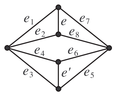
On the other hand, let $G$ be $K_{5}$, $K_{3,3}$ or $D_{4}$, where $D_{4}$ is the graph as illustrated in Fig. 2.2. Let $\omega:\Gamma(G)\to{\mathbb{Z}}$ be a map defined by

if $G=K_{5}$,

if $G=K_{3,3}$ and

if $G=D_{4}$. For a spatial embedding $f$ of $G$, an integer $\alpha_{\omega}(f)$ defined by

is called the $\alpha$-invariant of $f$ [18]. Then the following holds.

First we give a proof of Theorem 1-3. We can see that there exist exactly ten subgraphs $H_{1},H_{2},\ldots,H_{10}$ of $K_{6}$ each of which is isomorphic to $K_{3,3}$, exactly six subgraphs $G_{1},G_{2},\ldots,G_{6}$ of $K_{6}$ each of which is isomorphic to $K_{5}$ and exactly ten pairs of disjoint $3$-cycles $\lambda_{1},\lambda_{2},\ldots,\lambda_{10}$ of $K_{6}$. Then we have the following.

Next we give a proof of Theorem 1-4. In the following we denote a path of length $2$ of $K_{7}$ consisting of two edges $\overline{ij}$ and $\overline{jk}$ by $\overline{ijk}$, and the subgraph of $K_{7}$ obtained from $K_{7}$ by deleting the vertex $i$ and all of the edges incident to $i$ by $K_{6}^{(i)}\ (i=1,2,\ldots,7)$. Actually $K_{6}^{(i)}$ is isomorphic to $K_{6}$ for any $i$.

References

• [1] C. C. Adams, B. M. Brennan, D. L. Greilsheimer and A. K. Woo, Stick numbers and composition of knots and links, J. Knot Theory Ramifications 6 (1997), 149–161.
• [2] D. Bar-Natan, On the Vassiliev knot invariants, Topology 34 (1995), 423–472.
• [3] A. F. Brown, Embeddings of graphs in E3E^{3}, Ph. D. Dissertation, Kent State University, 1977.
• [4] J. H. Conway and C. McA. Gordon, Knots and links in spatial graphs, J. Graph Theory 7 (1983), 445–453.
• [5] T. Fleming and B. Mellor, Counting links in complete graphs, Osaka J. Math. 46 (2009), 173–201.
• [6] Y. Huh and C. Jeon, Knots and links in linear embeddings of K6K_{6}, J. Korean Math. Soc. 44 (2007), 661–671.
• [7] L. H. Kauffman, Formal knot theory, Mathematical Notes, 30. Princeton University Press, Princeton, NJ, 1983.
• [8] A. Mater, Stick numbers of links with two trivial components, Summer 2002 Knot Theory Projects, Department of Mathematics, California State University, San Bernardino.
• [9] T. Motohashi and K. Taniyama, Delta unknotting operation and vertex homotopy of graphs in R3R^{3}, KNOTS ’96 (Tokyo), 185–200, World Sci. Publ., River Edge, NJ, 1997.
• [10] H. Murakami, Vassiliev invariants of type two for a link, Proc. Amer. Math. Soc. 124 (1996), 3889–3896.
• [11] S. Negami, Ramsey theorems for knots, links and spatial graphs, Trans. Amer. Math. Soc. 324 (1991), 527–541.
• [12] R. Nikkuni, The second skew-symmetric cohomology group and spatial embeddings of graphs, J. Knot Theory Ramifications 9 (2000), 387–411.
• [13] R. Nikkuni and K. Taniyama, Symmetries of spatial graphs and Simon invariants, preprint. (arXiv:math.GT/0708.0066)
• [14] Y. Ohyama and K. Taniyama, Vassiliev invariants of knots in a spatial graph, Pacific J. Math. 200 (2001), 191–205.
• [15] J. L. Ramírez Alfonsín, Spatial graphs and oriented matroids: the trefoil, Discrete Comput. Geom. 22 (1999), 149–158.
• [16] R. A. Robertello, An invariant of knot cobordism, Comm. Pure Appl. Math. 18 (1965), 543–555.
• [17] M. Suzuki, Classification of the spatial-graph homology classes of a complete graph (in Japanese), Master Thesis, Tokyo Denki University, 1996.
• [18] K. Taniyama, Link homotopy invariants of graphs in R3R^{3}, Rev. Mat. Univ. Complut. Madrid 7 (1994), 129–144.
• [19] K. Taniyama, Cobordism, homotopy and homology of graphs in R3R^{3}, Topology 33 (1994), 509–523.
• [20] K. Taniyama and A. Yasuhara, Realization of knots and links in a spatial graph, Topology Appl. 112 (2001), 87–109.
• [21] V. A. Vassiliev, Cohomology of knot spaces, Theory of singularities and its applications, 23–69, Adv. Soviet Math., 1, Amer. Math. Soc., Providence, RI, 1990.