An entire transcendental family with a persistent Siegel disc

Rubén Berenguel ^†^†thanks: Email: ruben@maia.ub.es Núria Fagella ^†^†thanks: Email: fagella@maia.ub.es

Abstract

We study the class of entire transcendental maps of finite order with one critical point and one asymptotic value, which has exactly one finite pre-image, and having a persistent Siegel disc. After normalisation this is a one parameter family $f_{a}$ with $a\in\mathbb{C}^{*}$ which includes the semi-standard map $\lambda ze^{z}$ at $a=1$ , approaches the exponential map when $a\to 0$ and a quadratic polynomial when $a\to\infty$ . We investigate the stable components of the parameter plane (capture components and semi-hyperbolic components) and also some topological properties of the Siegel disc in terms of the parameter.

1 Introduction

Given a holomorphic endomorphism $f:S\to S$ on a Riemann surface $S$ we consider the dynamical system generated by the iterates of $f$ , denoted by $f^{n}=f\circ\stackrel{{\scriptstyle n}}{{\cdots}}\circ f$ . The orbit of an initial condition $z_{0}\in S$ is the sequence $\mathcal{O}^{+}(z_{0})=\{f^{n}(z_{0})\}_{n\in\mathbb{N}}$ and we are interested in classifying the initial conditions in the phase space or dynamical plane $S$ , according to the asymptotic behaviour of their orbits when $n$ tends to infinity.

There is a dynamically natural partition of the phase space $S$ into the Fatou set $\curv{F}(f)$ (open) where the iterates of $f$ form a normal family and the Julia set $\curv{J}(f)=S\backslash\curv{F}(f)$ which is its complement (closed).

If $S=\widehat{\mathbb{C}}=\mathbb{C}\cup\infty$ then $f$ is a rational map. If $S=\mathbb{C}$ and $f$ does not extend to the point at infinity, then $f$ is an entire transcendental map, that is, infinity is an essential singularity. Entire transcendental functions present many differences with respect to rational maps.

One of them concerns the singularities of the inverse function. For a rational map, all branches of the inverse function are well defined except at a finite number of points called the critical values, points $w=f(c)$ where $f^{\prime}(c)=0$ . The point $c$ is then called a critical point. If $f$ is an entire transcendental map, there is another possible obstruction for a branch of the inverse to be well defined, namely its asymptotic values. A point $v\in\mathbb{C}$ is called an asymptotic value if there exists a path $\gamma(t)\to\infty$ when $t\to\infty$ , such that $f(\gamma(t))\to v$ as $t\to\infty$ . An example is $v=0$ for $f(z)=e^{z}$ , where $\gamma(t)$ can be chosen to be the negative real axis.

In any case, the set of singularities of the inverse function, also called singular values, plays a very important role in the theory of iteration of holomorphic functions. This statement is motivated by the non-trivial fact that most connected components of the Fatou set (or stable set) are somehow associated to a singular value. Therefore, knowing the behaviour of the singular orbits provides information about the nature of the stable orbits in the phase space.

The dynamics of rational maps are fairly well understood, given the fact that they possess a finite number of critical points and hence of singular values. This motivated the definition and study of special classes of entire transcendental functions like, for example, the class $\mathcal{S}$ of functions of finite type which are those with a finite number of singular values. A larger class is $\mathcal{B}$ the class of functions with a bounded set of singularities. These functions share many properties with rational maps, one of the most important is the fact that every connected component of the Fatou set is eventually periodic (see e.g. [7] or [11]). There is a classification of all possible periodic connected components of the Fatou set for rational maps or for entire transcendental maps in class $\mathcal{S}$ . Such a component can only be part of a cycle of rotation domains (Siegel discs) or part of the basin of attraction of an attracting, super-attracting or parabolic periodic orbit.

We are specially interested in the case of rotation domains. We say that $\Delta$ is an invariant Siegel disc if there exists a conformal isomorphism $\varphi:\Delta\to\mathbb{D}$ which conjugates $f$ to $\mathcal{R}_{\theta}(z)=e^{2\pi i\theta}z$ (and $\varphi$ can not be extended further), with $\theta\in\mathbb{R}\setminus\mathbb{Q}\cap(0,1)$ called the rotation number of $\Delta$ . Therefore a Siegel disc is foliated by invariant closed simple curves, where orbits are dense. The existence of such Fatou components was first settled by Siegel [24] who showed that if $z_{0}$ is a fixed point of multiplier $\rho=f^{\prime}(z_{0})=e^{2\pi i\theta}$ and $\theta$ satisfies a Diophantine condition, then $z_{0}$ is analytically linearisable in a neighbourhood or, equivalently, $z_{0}$ is the centre of a Siegel disc. The Diophantine condition was relaxed later by Brjuno and Rüssman (for an account of these proofs see e.g. [17]), who showed that the same is true if $\theta$ belonged to the set of Brjuno numbers $\mathcal{B}$ . The relation of Siegel discs with singular orbits is as follows. Clearly $\Delta$ cannot contain critical points since the map is univalent in the disc. Instead, the boundary of $\Delta$ must be contained in the post-critical set $\cup_{c\in\mathrm{Sing}(f^{-1})}\overline{\mathcal{O}^{+}(c)}$ i.e., the accumulation set of all singular orbits. In fact something stronger is true, namely that $\partial\Delta$ is contained in the accumulation set of the orbit of at least one singular value (see [15]).

Our goal in this paper is to describe the dynamics of the one parameter family of entire transcendental maps

f_{a}(z)=\lambda a(e^{z/a}(z+1-a)-1+a),

where $a\in\mathbb{C}\setminus\{0\}=\mathbb{C}^{*}$ and $\lambda=e^{2\pi i\theta}$ with $\theta$ being a fixed irrational Brjuno number. Observe that $0$ is a fixed point of multiplier $\lambda$ and therefore, for all values of the parameter $a$ , there is a persistent Siegel disc $\Delta_{a}$ around $z=0$ . The functions $f_{a}$ have two singular values: the image of the only critical point $w=-1$ and an asymptotic value at $v_{a}=\lambda a(a-1)$ which has one and only one finite pre-image at the point $p_{a}=a-1$ .

The motivation for studying this family of maps is manifold. On one hand this is the simplest family of entire transcendental maps having one simple critical point and one asymptotic value with a finite pre-image (see Theorem 3.18 for the actual characterisation of $f_{a}$ ). The persistent Siegel disc makes it into a one-parameter family, since one of the two singular orbits must be accumulating on the boundary of $\Delta_{a}$ . We will see that the situation is very different, depending on which of the two singular values is doing that. Therefore, these maps could be viewed as the transcendental version of cubic polynomials with a persistent invariant Siegel disc, studied by Zakeri in [28]. In our case, many new phenomena are possible with respect to the cubic situation, like unbounded Siegel discs for example; but still the two parameter planes share many features like the existence of capture components or semi-hyperbolic ones.

There is a second motivation for studying the maps $f_{a}$ , namely that this one parameter family includes in some sense three emblematic examples. For $a=1$ we have the function $f_{1}(z)=\lambda ze^{z}$ , for large values of $a$ we will see that $f_{a}$ is polynomial-like of degree 2 in a neighbourhood of the origin (see Theorem 3.19); finally when $a\to 0$ , the dynamics of $f_{a}$ are approaching those of the exponential map $u\mapsto\lambda(e^{u}-1)$ , as it can be seen changing variables to $u=z/a$ . Thus the parameter plane of $f_{a}$ can be thought of as containing the polynomial $\lambda(z+\frac{z^{2}}{2})$ at infinity, its transcendental analogue $f_{1}$ at $a=1$ , and the exponential map at $a=0$ . The maps $z\mapsto\lambda ze^{z}$ have been widely studied (see [10] and [8]), among other reasons, because they share many properties with quadratic polynomials: in particular it is known that when $\theta$ is of constant type, the boundary of the Siegel disc is a quasi-circle that contains the critical point. It is not known however whether there exist values of $\theta$ for which the Siegel disc of $f_{1}$ is unbounded. In the long term we hope that this family $f_{a}$ can throw some light into this and other problems about $f_{1}$ .

For the maps at hand we prove the following.

Theorem A.

a)

There exists $R,M>0$ such that if $\theta$ is of constant type and $|a|>M$ then the boundary of $\Delta_{a}$ is a quasi-circle which contains the critical point. Moreover $\Delta_{a}\subset D(0,R)$ .
b)

If $\theta$ is Diophantine and the orbit of $c=-1$ belongs to a periodic basin or is eventually captured by the Siegel disc, then either the Siegel disc $\Delta_{a}$ is unbounded or its boundary is an indecomposable continuum.
c)

If $\theta$ is Diophantine and $f_{a}^{n}(-1)\stackrel{{\scriptstyle n\to\infty}}{{\longrightarrow}}\infty$ the Siegel disc $\Delta_{a}$ is unbounded, and the boundary contains the asymptotic value.

Part a) follows from Theorem 3.19 (see Corollary 1 below it). The remaining parts (Theorem 3.20) are based on Herman’s proof [12] of the fact that Siegel discs of the exponential map are unbounded, if the rotation number is Diophantine, although in this case there are some extra difficulties given by the free critical point and the finite pre-image of the asymptotic value.

In this paper we are also interested in studying the parameter plane of $f_{a}$ , which is $\mathbb{C}^{*}$ , and in particular the connected components of its stable set, i.e., the parameter values for which the iterates of both singular values form a normal family in some neighbourhood. We denote this set as $\mathcal{S}$ (not to be confused with the class of finite type functions). These connected components are either capture components, where an iterate of the free singular value falls into the Siegel disc; or semi-hyperbolic, when there exists an attracting periodic orbit (which must then attract the free singular value); otherwise they are called queer.

The following theorem summarises the properties of semi-hyperbolic components, and is proved in Section 4 (see Proposition 4, Theorems 4.22, 4.23 and Proposition 5 therein). By a component of a set we mean a connected component.

Theorem B.

Define

	$\displaystyle H^{c}$	$\displaystyle=\{a\in\mathbb{C}\|\mathcal{O}^{+}(-1)\textrm{ is attracted to an attracting periodic orbit}\},$
	$\displaystyle H^{v}$	$\displaystyle=\{a\in\mathbb{C}\|\mathcal{O}^{+}(v_{a})\textrm{ is attracted to an attracting periodic orbit}\}.$

a)

Every component of $H^{v}\cup H^{c}$ is simply connected.
b)

If $W$ is a component of $H^{v}$ then $W$ is unbounded and the multiplier map $\chi:W\to\mathbb{D}^{*}$ is the universal covering map.
c)

There is one component $H_{1}^{v}$ of $H^{v}$ for which $\mathcal{O}^{+}(v_{a})$ tends to an attracting fixed point. $H_{1}^{v}$ contains the segment $[r,\infty)$ for $r$ large enough.
d)

If $W$ is a component of $H^{c}$ , then $W$ is bounded and the multiplier map $\chi:W\to\mathbb{D}$ is a conformal isomorphism.

Indeed, when the critical point is attracted by a cycle, we naturally see copies of the Mandelbrot set in parameter space. Instead, when it is the asymptotic value that acts in a hyperbolic fashion, we find unbounded exponential-like components, which can be parametrised using quasi-conformal surgery.

A dichotomy also occurs with capture components. Numerically we can observe copies of quadratic Siegel discs in parameter space, which correspond to components for which the asymptotic value is being captured. There is in fact a main capture component $C_{0}^{v}$ , the one containing $a=1$ (see Figure 1), which corresponds to parameters for which the asymptotic value $v_{a}$ , belongs itself to the Siegel disc. This is possible because of the existence of a finite pre-image of $v_{a}$ . The centre of $C_{0}^{v}$ is the semi-standard map $f_{1}(z)=\lambda ze^{z}$ , for which zero itself is the asymptotic value.

The properties we show for capture components are summarised in the following theorem (see Section 5: Theorem 5.24 and Proposition 7).

Theorem C.

Let us define

	$\displaystyle C^{c}$	$\displaystyle=\{a\in\mathbb{C}\|f_{a}^{n}(-1)\in\Delta_{a}\textrm{ for some }n\geq 1\},$
	$\displaystyle C^{v}$	$\displaystyle=\{a\in\mathbb{C}\|f_{a}^{n}(v_{a})\in\Delta_{a}\textrm{ for some }n\geq 0\}.$

Then

a)

$C^{c}$ and $C^{v}$ are open sets.
b)

Every component $W$ of $C^{c}\cup C^{v}$ is simply connected.
c)

Every component $W$ of $C^{c}$ is bounded.
d)

There is only one component of $C_{0}^{v}=\{a\in\mathbb{C}|v_{a}\in\Delta_{a}\}$ and it is bounded.

Numerical experiments show that if $\theta$ is of constant type, the boundary of $C_{0}^{v}$ is a Jordan curve, corresponding to those parameter values for which both singular values lie on the boundary of the Siegel disc (see Figure 1). This is true for the slice of cubic polynomials having a Siegel disc of rotation number $\theta$ , as shown by Zakeri in [28], but his techniques do not apply to this transcendental case.

Refer to caption — Figure 1: Left: Simple escape time plot of the parameter plane. Light grey: asymptotic orbit escapes, dark grey critical orbit escapes, white neither escapes. Regions labelled $H_{1}$ and $H_{2}$ correspond to parameters for which the asymptotic value is attracted to an attracting cycle. Right: The same plot, using a different algorithm which emphasises the capture components. Upper left: $(-2,2),$ Lower right: $(4,-4)$ .

As we already mentioned, we are also interested in parameter values for which $f_{a}$ is Julia stable, i.e. where both families of iterates $\{f_{a}^{n}(-1)\}_{n\in\mathbb{N}}$ and $\{f_{a}^{n}(v_{a})\}_{n\in\mathbb{N}}$ are normal in a neighbourhood of $a$ (see Section 6). We first show that any parameter in a capture component or a semi-hyperbolic component is $\mathcal{J}$ -stable.

Proposition 1.

If $a\in H\cup C$ then $f_{a}$ is $\mathcal{J}$ -stable, where $H=H^{c}\cup H^{v}$ and $C=C^{c}\cup C^{v}$ .

By using holomorphic motions and the proposition above, it is enough to have certain properties for one parameter value $a_{0}$ , to be able to “extend” them to all parameters belonging to the same stable component. More precisely we obtain the following corollaries (see Proposition 8 and Corollary 3).

Proposition 2.

a)

If $\theta$ is of constant type and $a\in C_{0}^{v}$ (i.e. the asymptotic value lies inside the Siegel disc) then $\partial\Delta_{a}$ is a quasi-circle that contains the critical point.
b)
Let $W\subset H^{v}\cup C^{v}$ be a component intersecting $\{|z|>M\}$ where $M$ is as in Theorem A. Then,
1. i)
  
  if $\theta$ is of constant type, for all $a\in W$ the boundary $\partial\Delta_{a}$ is a quasi-circle containing the critical point.
2. ii)
  
  There exist values of $\theta\in\mathbb{R}\backslash\mathbb{Q}\cap(0,1)$ such that if a component $W\subset C^{v}\cup H^{v}$ intersects $\{|z|>M\}$ , then for all $a\in W$ , the boundary of $\Delta_{a}$ is a quasi-circle not containing the critical point.

The paper is organised as follows. Section 2 contains statements and references of some of the results used throughout the paper. Section 3 contains the characterisation of the family $f_{a}$ , together with descriptions and images of the possible scenarios in dynamical plane. It also contains the proof of Theorem A. Section 4 deals with semi-hyperbolic components and contains the proof of Theorem B, split in several parts, and not necessarily in order. In the same fashion, capture components and Theorem C are treated in Section 5. Finally Section 6 investigates Julia stability and contains the proofs of Propositions D and E.

2 Preliminary results

In this section we state results and definitions which will be useful in the sections to follow.

2.1 Quasi-conformal mappings and holomorphic motions

First we introduce the concept of quasi-conformal mapping. Quasi-conformal mappings are a very useful tool in complex dynamical systems as they provide a bridge between a geometric construction for a system and its analytic information. They are also a fundamental pillar for the framework of quasi-conformal surgery, the other one being the measurable Riemann mapping theorem. For the groundwork on quasi-conformal mappings see for example [1], and for an exhaustive account on quasi-conformal surgery, see [4].

Definition 1.

Let $\mu:U\subseteq\mathbb{C}\to\mathbb{C}$ be a measurable function. Then it is a $k$ -Beltrami form (or Beltrami coefficient, or complex dilatation) of $U$ if $\|\mu(z)\|_{\infty}\leq k<1$ .

Definition 2.

Let $f:U\subseteq\mathbb{C}\to V\subseteq\mathbb{C}$ be a homeomorphism. We call it $k$ -quasi-conformal if locally it has distributional derivatives in $\mathcal{L}^{2}$ and

\displaystyle\mu_{f}(z)=\frac{\frac{\mathrm{\partial}f}{\mathrm{\partial}\bar{z}}(z)}{\frac{\mathrm{\partial}f}{\mathrm{\partial}z}(z)}

(1)

is a $k$ -Beltrami coefficient. Then $\mu_{f}$ is called the complex dilatation of $f(z)$ (or the Beltrami coefficient of $f(z)$ ).

Given $f(z)$ satisfying all above except being an homeomorphism, we call it $k$ -quasi-regular.

The following technical theorem will be used when we have compositions of quasi-conformal mappings and finite order mappings.

Theorem 2.4 ([9, p. 750]).

A $k$ -quasi-conformal mapping in a domain $U\subset\mathbb{C}$ is uniformly Hölder continuous with exponent $(1-k)/(1+k)$ in every compact subset of $U$ .

Theorem 2.5 ((Measurable Riemann Mapping, MRMT)).

Let $\mu$ be a Beltrami form over $\mathbb{C}$ . Then there exists a quasi-conformal homeomorphism $f$ integrating $\mu$ (i.e. the Beltrami coefficient of $f$ is $\mu$ ), unique up to composition with an affine transformation.

Theorem 2.6 ((MRMT with dependence of parameters)).

Let $\Lambda$ be an open set of $\mathbb{C}$ and let $\{\mu_{\lambda}\}_{\lambda\in\Lambda}$ be a family of Beltrami forms on $\mathbb{\hat{C}}$ . Suppose $\lambda\to\mu_{\lambda}(z)$ is holomorphic for each fixed $z\in\mathbb{C}$ and $\|\mu_{\lambda}\|_{\infty}\leq k<1$ for all $\lambda$ . Let $f_{\lambda}$ be the unique quasi-conformal homeomorphism which integrates $\mu_{\lambda}$ and fixes three given points in $\mathbb{\hat{C}}$ . Then for each $z\in\mathbb{\hat{C}}$ the map $\lambda\to f_{\lambda}(z)$ is holomorphic.

The concept of holomorphic motion was introduced in [14] along with the (first) $\lambda$ -lemma.

Definition 3.

Let $h:\Lambda\times X_{0}\to\mathbb{\hat{C}},$ where $\Lambda$ is a complex manifold and $X_{0}$ an arbitrary subset of $\mathbb{\hat{C}}$ , such that

•

$h(0,z)=z$ ,
•

$h(\lambda,\cdot)$ is an injection from $X_{0}$ to $\mathbb{\hat{C}}$ ,
•

For all $z\in X_{0}$ , $z\mapsto h(\lambda,z)$ is holomorphic.

Then $h_{\lambda}(z)=h(\lambda,z)$ is called a holomorphic motion of $X$ .

The following two fundamental results can be found in [14] and [25] respectively.

Lemma 1 ((First $\lambda$ -lemma)).

A holomorphic motion $h_{\lambda}$ of any set $X\subset\mathbb{\hat{C}}$ extends to a jointly continuous holomorphic motion of $\bar{X}$ .

Lemma 2 ((Second $\lambda$ -lemma)).

Let $U\subset\mathbb{C}$ be a set and $h_{\lambda}$ a holomorphic motion of $U$ . This motion extends to a holomorphic motion of $\mathbb{C}$ .

2.2 Hadamard’s factorisation theorem

We will need the notion of rank and order to be able to state Hadamard’s factorisation theorem, which we will use in the proof of Theorem 3.18. All these results can be found in [5].

Definition 4.

Given $f:\mathbb{C}\to\mathbb{C}$ an entire function we say it is of finite order if there are positive constants $a>0$ , $r_{0}>0$ such that

|f(z)|<e^{|z|^{a}},\quad\text{for }|z|>r_{0}.

Otherwise, we say $f(z)$ is of infinite order. We define

\lambda=\inf\{a||f(z)|<\mathrm{exp}(|z|^{a})\text{ for }|z|\text{ large enough}\}

as the order of $f(z)$ .

Definition 5.

Let $f:\mathbb{C}\to\mathbb{C}$ be an entire function with zeroes $\{a_{1},a_{2},\ldots\}$ counted according to multiplicity. We say $f$ is of finite rank if there is an integer $p$ such that

\displaystyle\sum_{n=1}^{\infty}|a_{n}|^{p+1}<\infty.

(2)

We say it is of rank $p$ if $p$ is the smallest integer verifying (2). If $f$ has a finite number of zeroes then it has rank 0 by definition.

Definition 6.

An entire function $f:\mathbb{C}\to\mathbb{C}$ is said to be of finite genus if it has finite rank $p$ and it factorises as:

\displaystyle f(z)=z^{m}e^{g(z)}\cdot\prod_{n=1}^{\infty}E_{p}(z/a_{n}),

(3)

where $g(z)$ is a polynomial, $a_{n}$ are the zeroes of $f(z)$ as in the previous definition and

E_{p}(z)=(1-z)e^{z+\frac{z^{2}}{2}+\ldots+\frac{z^{p}}{p}}.

We define the genus of $f(z)$ as $\mu=\max\{\mathrm{deg}\,g,\mathrm{rank}\,f\}$

Theorem 2.7.

If $f$ is an entire function of finite genus $\mu$ then $f$ is of finite order $\lambda<\mu+1$ .

The converse of this theorem is also true, as we see below.

Theorem 2.8 ((Hadamard’s factorisation)).

Let $f$ be an entire function of finite order $\lambda$ . Then $f$ is of finite genus $\mu\leq\lambda$ .

Observe that Hadamard’s factorisation theorem implies that every entire function of finite order can be factorised as in (3).

2.3 Siegel discs

The following theorem (which is an extension of the original theorem by C.L. Siegel) gives arithmetic conditions on the rotation number of a fixed point to ensure the existence of a Siegel disc around it. J-C. Yoccoz proved that this condition is sharp in the quadratic family. The proof of this theorem can be found in [17].

Theorem 2.9 ((Brjuno-Rüssmann)).

Let $f(z)=\lambda z+\mathcal{O}(z^{2})$ . If $\frac{p_{n}}{q_{n}}=[a_{1};a_{2},\ldots,a_{n}]$ is the $n$ -th convergent of the continued fraction expansion of $\theta$ , where $\lambda=e^{2\pi i\theta}$ , and

\displaystyle\sum_{n=0}^{\infty}\frac{\log(q_{n+1})}{q_{n}}<\infty,

(4)

then $f$ is locally linearisable.

Irrational numbers with this property are called of Brjuno type.

We define the notion of conformal capacity as a measure of the “size” of Siegel discs.

Definition 7.

Consider the Siegel disc $\Delta$ and the unique linearising map $h:\mathbb{D}(0,r)\stackrel{{\scriptstyle\sim}}{{\to}}\Delta$ , with $h(0)$ and $h^{\prime}(0)=1$ . The radius $r>0$ of the domain of $h$ is called the conformal capacity of $\Delta$ and is denoted by $\kappa(\Delta)$ .

A Siegel disc of capacity $r$ contains a disc of radius $\frac{r}{4}$ by Koebe 1/4 Theorem.

The following theorem (see [26] for a proof) shows that Siegel discs can not shrink indefinitely.

Theorem 2.10.

Let $0<\theta<1$ be an irrational number of Brjuno type, and let $\Phi(\theta)=\sum_{n=1}^{\infty}(\log q_{n+1}/q_{n})<\infty$ be the Brjuno function. Let $S(\theta)$ be the space of all univalent functions $f:\mathbb{D}\to\mathbb{C}$ with $f(0)=0$ and $f^{\prime}(0)=e^{2\pi i\theta}$ . Finally, define $\kappa(\theta)=\inf_{f\in S(\theta)}\kappa(\Delta_{f})$ , where $\kappa(\Delta)$ is the conformal capacity of $\Delta$ . Then, there is a universal constant $C>0$ such that $|\log(\kappa(\theta))+\Phi(\theta)|<C$ .

We will also need a well-known theorem about the regularity of the boundary of Siegel discs of quadratic polynomials. Its proof can be found in [6].

Theorem 2.11 ((Douady-Ghys)).

Let $\theta$ be of bounded type, and $p(z)=e^{2\pi i\theta}z+z^{2}$ . Then the boundary of the Siegel disc around 0 is a quasi-circle containing the critical point.

The following is a theorem by M. Herman concerning critical points on the boundary of Siegel discs. Its proof can be found in [12, p. 601]

Theorem 2.12 ((Herman)).

Let $g(z)$ be an entire function such that $g(0)=0$ and $g^{\prime}(0)=e^{2\pi i\alpha}$ with $\alpha$ Diophantine. Let $\Delta$ be the Siegel disc around $z=0$ . If $\Delta$ has compact closure in $\mathbb{C}$ and $\left.g\right|_{\bar{\Delta}}$ is injective then $g(z)$ has a critical point in $\partial\Delta$ .

In fact, the set of Diophantine numbers could be replaced by the set $\mathcal{H}$ of Herman numbers, where $\mathcal{D}\subsetneq\mathcal{H}\subsetneq\mathcal{B}$ , as shown in [27].

Finally, we state a result which is a combination of Theorems 1 and 2 in [20].

Definition 8.

We define the class $\mathcal{B}$ as the class of entire functions with a bounded set of singular values.

Theorem 2.13 ((Rempe), [19]).

Let $f\in\mathcal{B}$ with $S(f)\subset\curv{J}(f)$ , where $S(f)$ denotes the set of singular values of $f$ . If $\Delta$ is a Siegel disc of $f(z)$ which is unbounded, then $S(f)\cap\partial\Delta\neq\emptyset$ .

2.4 Topological results

To prove Theorem 3.20 we need to extend a result of Rogers in [21] to a larger class of functions, namely functions of finite order with no wandering domains.

The result we need follows some preliminary definitions.

Definition 9.

A continuum is a compact connected non-void metric space.

Definition 10.

A pair $(g,\Delta)$ is a local Siegel disc if $g$ is conformally conjugate to an irrational rotation on $\Delta$ and $g$ extends continuously to $\bar{\Delta}$ .

Definition 11.

We say a bounded local Siegel disc $(\left.f\right|_{\Delta},\Delta)$ is irreducible if the boundary of $\Delta$ separates the centre of the disc from $\infty$ , but no proper closed subset of the boundary of $\Delta$ has this property.

Theorem 2.14.

Suppose $\Delta$ is a Siegel disc of a function $f$ in the class $\mathcal{B}$ , and $\partial\Delta$ is a decomposable continuum. Then $\partial\Delta$ separates $\mathbb{C}$ into exactly two complementary domains.

For the proof of this theorem we will need the following ingredients which will be only used in this proof. The topological results can be found in any standard reference on algebraic topology.

Theorem 2.15.

If $(\Delta,f_{\theta})$ is a bounded irreducible local Siegel disc, then the following are equivalent:

•

$\partial\Delta$ is a decomposable continuum,
•

each pair of impressions is disjoint, and
•

the inverse of the map $\varphi:\mathbb{D}\to\Delta$ extends continuously to a map $\Psi:\partial$ $\Delta\to S^{1}$ such that for each $\eta\in S^{1}$ , the fibre $\Psi^{-1}(\eta)$ is the impression $I(\eta)$ .

Proof.

See [21].

∎

Theorem 2.16 ((Vietoris-Begle)).

Let $X$ and $Y$ be compact metric spaces and $f:X\to Y$ continuous and surjective and suppose that the fibres are acyclic, i.e.

\tilde{H}^{r}(f^{-1}(y))=0,0\leq r\leq n-1,\quad\forall y\in Y,

where $\tilde{H}^{r}$ denotes the $r$ -th reduced co-homology group. Then, the induced homomorphism

f^{*}:\tilde{H}^{r}(Y)\to\tilde{H}^{r}(X)

is an isomorphism for $r\leq n-1$ and is a surjection for $r=n$ .

Theorem 2.17 ((Alexander’s duality)).

Let $X$ be a compact sub-space of the Euclidean space $E$ of dimension $n$ , and $Y$ its complement in $E$ . Then,

\tilde{H}_{q}(X)\cong\tilde{H}^{n-q-1}(Y)

where $\tilde{H}_{*},\,\tilde{H}^{*}$ stands for Čech reduced homology and reduced co-homology respectively.

Remark 1.

The case $E=S^{2}$ , $X=S^{1}$ (or $H^{1}(X)=\mathbb{Z}$ ) is Jordan’s Curve Theorem.

Definition 12.

If $X$ is a compact subset of $\mathbb{C}$ , then the three following conditions are equivalent:

•

$X$ is cellular,
•

$X$ is a continuum that does not separate $\mathbb{C}$ ,
•

$H^{1}(X)=0=\tilde{H}^{0}(X)$ ,

where $\tilde{H}^{r}(X)$ stands for reduced Čech co-homology and $H^{r}(X)$ for Čech co-homology.

Definition 13.

We say a map $f:X\to Y$ is cellular if each fibre $f^{-1}(y)$ is a cellular set.

Remark 2.

Recall that $\tilde{H}^{1}(X)\cong H^{1}(X)$ .

Remark 3.

By definition and in view of the Vietoris-Begle Theorem, cellular maps induce isomorphisms between first reduced co-homology groups.

Proof of Theorem 2.14.

We first show that any Siegel disc $\Delta$ for $f\in\mathcal{B}$ is a bounded irreducible local Siegel disc. Recall that we define the escaping set of a function $f:\mathbb{C}\to\mathbb{C}$ as:

I(f)=\{z|\,f^{n}(z)\to\infty\textrm{ as }n\to\infty\}.

Clearly $(\left.f\right|_{\Delta},\Delta)$ is a local Siegel disc. It is also bounded by assumption. The only thing left to prove is it is irreducible. If $X$ is a proper closed subset of $\partial\Delta$ and if $x$ is a point of $\partial\Delta\backslash X$ , then there is a small disc $B$ containing $x$ and missing $X$ . Since $x\in\partial\Delta$ , the disc $B$ contains a point of $\Delta$ . As $x\in\partial\Delta\subset\curv{J}(f)$ , the disc $B$ contains a point $y\in I(f)$ . Now, Theorem 3.1.1 in [23] states that for $f\in\mathcal{B}$ the set $I(f)\cup\{\infty\}$ is arc-connected, and thus $y$ can be arc-connected to $\infty$ through points in $I(f)$ . It follows that the centre of the Siegel disc and infinity are in the same complementary domain of $\mathbb{C}\backslash X$ .

Clearly $\Psi(\eta)$ for $\eta\in S^{1}$ is a continuum, which is called the impression of $\eta$ and denoted $\mathrm{Imp}(\eta).$ Furthermore, $\mathrm{Imp}(\eta)$ does not separate $\mathbb{C}$ . Indeed, if $U$ is a bounded complementary domain of $\mathrm{Imp}(\eta)$ , then either $f^{n}(U)\cap U=\emptyset$ for all $n$ or there are intersection points. Clearly $f^{n}(U)\cap U=\emptyset$ , as if $f^{n}(U)\cap U\neq\emptyset$ for some $n$ , then $f^{n}(\partial U)\cap\partial U\neq\emptyset$ , but this implies $\mathrm{Imp}(\eta)=F^{n}(\mathrm{Imp}(\eta))=\mathrm{Imp}(\eta+n\theta)$ and as $\partial\Delta$ is a decomposable continuum, each pair of impressions is disjoint by Theorem 2.15 and this intersection must be empty. Hence, $f^{n}(U)\cap U=\emptyset$ for all $n\in\mathbb{N}$ which implies $U$ is a wandering domain, and for functions in $\mathcal{B}$ it is known there are no wandering domains (see [7]).

Therefore $\mathrm{Imp}(\eta)$ is a cellular set and thus $\Psi$ is a cellular map. The Vietoris-Begle theorem implies that the induced homomorphism $\Psi^{*}:\tilde{H}^{1}(S^{1})\to\tilde{H}^{1}(\partial\Delta)$ is an isomorphism (see Remark 3). Then $\tilde{H}^{1}(\partial\Delta)=\mathbb{Z}$ and by Alexander’s duality $\partial\Delta$ separates $\mathbb{C}$ into exactly two complementary domains (see Remark 1).

∎

3 The (entire transcendental) family $f_{a}$

In this section we describe the dynamical plane of the family of entire transcendental maps

f_{a}(z)=\lambda a(e^{z/a}(z+1-a)-1+a),

for different values of $a\in\mathbb{C}^{*}$ , and for $\lambda=e^{2\pi i\theta}$ , with $\theta$ being a fixed irrational Brjuno number (unless otherwise specified). For these values of $\lambda$ , in view of Theorem 2.9 there exists an invariant Siegel disc around $z=0$ , for any value of $a\in\mathbb{C}^{*}$ .

We start by showing that this family contains all possible entire transcendental maps with the properties we require.

Theorem 3.18.

Let $g(z)$ be an entire transcendental function having the following properties

1.

finite order,
2.

one asymptotic value $v$ , with exactly one finite pre-image $p$ of $v$ ,
3.

a fixed point (normalised to be at 0) of multiplier $\lambda\in\mathbb{C}$ ,
4.

a simple critical point (normalised to be at $z=-1$ ) and no other critical points.

Then $g(z)=f_{a}(z)$ for some $a\in\mathbb{C}$ with $v=\lambda a(a-1)$ and $p=a-1$ . Moreover no two members of this family are conformally conjugate.

Proof.

As $g(z)-v=0$ has one solution at $z=p$ , we can write:

g(z)=(z-p)^{m}e^{h(z)}+v,

where, by Hadamard’s factorisation theorem (Theorem 2.8), $h(z)$ must be a polynomial, as $g(z)$ has finite order. The derivative of this function is

g^{\prime}(z)=e^{h(z)}(z-p)^{m-1}(m+(z-p)h^{\prime}(z)),

whose zeroes are the solutions of $z-p=0$ (if $m>1$ ) and the solutions of $m+(z-p)h^{\prime}(z)=0$ . But as the critical point must be simple and unique, $m=1$ and $\deg h^{\prime}(z)=0$ . Therefore

g(z)=(z-p)e^{\alpha z+\beta}+v,

and from the expression for the critical points,

\alpha=\frac{1}{p+1}.

Moreover from the fact that $g(0)=0$ we can deduce that $v=pe^{\beta}$ , and from condition 3, i.e. $g^{\prime}(0)=\lambda$ , we obtain $e^{\beta}=\lambda(1+p)$ . All together yields

g(z)=\lambda(z-p)(1+p)e^{z/(1+p)}+\lambda p(1+p).

Writing $a=p+1$ we arrive to

g(z)=\lambda a(z-a+1)e^{z/a}+\lambda a(a-1)=f_{a}(z),

as we wanted.

Finally, if $f_{a}(z)$ and $f_{a^{\prime}}(z)$ are conformally conjugate, the conjugacy must fix 0,-1 and $\infty$ and therefore is the identity map.

∎

3.1 Dynamical planes

For any parameter value $a\in\mathbb{C}^{*}$ , the Fatou set always contains the Siegel disc $\Delta_{a}$ and all its pre-images. Moreover, one of the singular orbits must be accumulating on the boundary of $\Delta_{a}$ . The other singular orbit may then either eventually fall in $\Delta_{a}$ , or accumulate in $\partial\Delta_{a}$ , or have some independent behaviour. In the first case we say that the singular value is captured by the Siegel disc. More precisely we define the capture parameters as

	$\displaystyle C=\{a\in\mathbb{C}^{*}\|$	$\displaystyle f_{a}^{n}(-1)\in\Delta_{a}\textrm{ for some }n\geq 1\textrm{ or }$
		$\displaystyle f_{a}^{n}(v_{a})\in\Delta_{a}\textrm{ for some }n\geq 0\}$

Naturally $C$ splits into two sets $C=C^{c}\cup C^{v}$ depending on whether the captured orbit is the critical orbit ( $C^{c}$ ) or the orbit of the asymptotic value ( $C^{v}$ ). We will follow this convention, superscript $c$ for critical and superscript $v$ for asymptotic, throughout this paper.

In the second case, that is, when the free singular value has an independent behaviour, it may happen that it is attracted to an attracting periodic orbit. We define the semi-hyperbolic parameters $H$ as

H=\{a\in\mathbb{C}^{*}|f_{a}\textrm{ has an attracting periodic orbit}\}.

Again this set splits into two sets, $H=H^{c}\cup H^{v}$ depending on whether the basin contains the critical point or the asymptotic value.

Notice that these four sets $C^{c},\,C^{v},\,H^{c},\,H^{v}$ are pairwise disjoint, since a singular value must always belong to the Julia set, as its orbit has to accumulate on the boundary of the Siegel disc.

In the following sections we will describe in detail these regions of parameter space, but let us first show some numerical experiments. For all figures we have chosen $\theta=\frac{1+\sqrt{5}}{2}$ , the golden mean number.

Figure 1 (in the Introduction) shows the parameter plane, where the left side is made with a simple escaping algorithm. The component containing $a=1$ is the main capture component for which $v_{a}$ itself belongs to the Siegel disc. On the right side we see the same parameters, drawn with a different algorithm. Also in Figure 1, we can partially see the sets $H^{v}_{1}$ and $H^{v}_{2}$ (and infinitely many others), where the sub-indices denote the period of the attracting orbit.

In Figure 2 (left) we can see the dynamical plane for $a$ chosen in one of the semi-hyperbolic components of Figure 1, where the Siegel disc and the attracting orbit and corresponding basin are shown in different colours.

Figure 2 (right) shows the dynamical plane of $f_{1}(z)=\lambda ze^{z}$ , the semi-standard map. In this case the asymptotic value $v_{1}=0$ is actually the centre of the Siegel disc. It is still an open question whether, for some exotic rotation number, this Siegel disc can be unbounded. For bounded type rotation numbers, as the one in the figure, the boundary is a quasi-circle and contains the critical point [10].

Figure 3, left side, shows a close-up view of the parameter region around $a=0$ , and in the right side, we can see a closer view of a random spot, in particular a region in $H^{c}$ , that is, parameters for which the critical orbit is attracted to a cycle.

One of these dynamical planes is shown in Figure 4. Observe that the orbit of the asymptotic value is now accumulating on $\partial\Delta_{a}$ and we may have unbounded Siegel discs.

Finally Figure 5 shows some components of $C^{v}$ , where the orbit of the asymptotic value is captured by the Siegel disc.

We start by considering large values of $a\in\mathbb{C}^{*}$ . By expanding $f_{a}(z)$ into a power series it is easy to check that as $a\to\infty$ the function approaches the quadratic polynomial $\lambda z(1+z/2)$ . It is therefore not surprising that we have the following theorem, which we shall prove at the end of this section.

Theorem 3.19.

There exists $M>0$ such that the entire transcendental family $f_{a}(z)$ is polynomial-like of degree two for $|a|>M$ . Moreover, the Siegel disc $\Delta_{a}$ (and in fact, the full small filled Julia set) is contained in a disc of radius $R$ where $R$ is a constant independent of $a$ .

Figure 6 shows the dynamical plane for $a=15+15i$ , $\lambda=e^{2\pi(\frac{1+\sqrt{5}}{2})i}$ where we clearly see the Julia set of the quadratic polynomial $\lambda z(1+z/2)$ , shown on the right side.

An immediate consequence of Theorem 3.19 above follows from Theorem 2.11. This is Part a) of Theorem A in the Introduction.

Corollary 1.

For $|a|>M$ , and $\theta$ of constant type the boundary of $\Delta_{a}$ is a quasi-circle that contains the critical point.

In fact we will prove in Section 5 (Proposition 8) that the same occurs in many other situations like, for example, when the asymptotic value lies itself inside the Siegel disc or when it is attracted to an attracting periodic orbit. See Figures 2 (Left) and 6.

In fact we believe that this family provides examples of Siegel discs with an asymptotic value on the boundary, but such that the boundary is a quasi-circle containing also the critical point. A parameter value with this property could be given by $a_{0}\approx 1.544913893+0.32322773i\in\partial C_{0}^{v}$ , $\lambda=e^{2\pi(\frac{1+\sqrt{5}}{2})i}$ (see Figure 7) where the asymptotic value and the critical point coincide.

The opposite case, that is, the Siegel disc being unbounded and its boundary non-locally connected also takes place for certain values of the parameter $a$ , as we show in the following theorem, which covers parts b) and c) of Theorem A (see Figure 8).

Theorem 3.20.

Let $\theta$ be Diophantine¹¹ 1 Diophantine numbers can actually be replaced by the larger class of irrational numbers $\mathcal{H}$ (see [27], [18]), then:

a)

If $f_{a}^{n}(-1)\to\infty$ then $\Delta_{a}$ is unbounded and $v_{a}\in\partial\Delta_{a}$ ,
b)

if $a\in H^{c}\cup C^{c}$ either $\Delta_{a}$ is unbounded or $\partial\Delta_{a}$ is an indecomposable continuum.

Proof.

The proof of the first part is a slight modification of Herman’s proof for the exponential map (see [12]). The difference is given by the fact that the asymptotic value of $f_{a}(z)$ is not an omitted value, and by the existence of a second singular value. For both parts we need the following definitions. Suppose that $\Delta:=\Delta_{a}$ is bounded and let $\Delta_{i}$ denote the bounded components of $\mathbb{C}\backslash\partial\Delta$ . Let $\Delta_{\infty}$ be the unbounded component. Since $\Delta$ and $\Delta_{i}$ are simply connected, then $\hat{\Delta}:=\mathbb{C}\backslash\Delta_{\infty}$ is compact and simply connected. By the Maximum Modulus Principle and Montel’s theorem, $\{\left.f_{a}^{n}\right|_{\Delta_{i}}\}_{n\in\mathbb{N}}$ form a normal family and hence $\Delta_{i}$ is a Fatou component. We also have that $\partial\Delta=\partial\Delta_{\infty}$ , although this does not imply a priori that $\Delta_{i}=\emptyset$ (see Wada lakes and similar examples [22]).

Proof of Part a).

Now suppose the critical orbit is unbounded. Then $c\in\mathcal{J}(f_{a})$ , but $\hat{\Delta}\cap\mathcal{J}(f_{a})$ is bounded and invariant. Hence $c\notin\hat{\Delta}$ .

We claim that there exists $U$ a simply connected neighbourhood of $\hat{\Delta}$ such that $U$ contains no singular values. Indeed, suppose that the asymptotic value $v_{a}$ belongs to $\hat{\Delta}$ . Since $v_{a}\in\mathcal{J}(f)$ , then $v_{a}\in\partial\Delta$ . But $\Delta$ is bounded, and $\left.f\right|_{\partial\Delta}$ is surjective, hence the only finite pre-image of $v_{a}$ , namely $a-1$ , also belongs to $\partial\Delta$ . This means that $v_{a}$ is not acting as an asymptotic value but as a regular point, since $f(z)$ is a local homeomorphism from $a-1$ to $v_{a}$ .

Hence there are no singular values in $U$ . It follows that

\left.f\right|_{f^{-1}(U)}:f^{-1}(U)\to U

is a covering and $f^{-1}:\Delta\to\Delta$ extends to a continuous map $h(z)$ from $\bar{\Delta}$ to $\bar{\Delta}$ . Since $hf=fh=id$ , it follows that $\left.f\right|_{\partial\Delta}$ is injective. As this mapping is always surjective, it is a homeomorphism. We now apply Herman’s main theorem in [12] (see Theorem 2.12) to conclude that $\partial\Delta$ must have a critical point, which contradicts our assumptions. It follows that $\Delta$ is unbounded. Finally Theorem 2.13 implies that $v_{a}\in\partial\Delta_{a}$ .

Proof of part b).

The work was done already when proving Theorem 2.14. Since $f_{a}$ has 2 singular values, it belongs to the Eremenko-Lyubich class $\mathcal{B}$ . Hence, if we assume that $\Delta_{a}$ is bounded, it follows from Theorem 2.14 that $\partial\Delta_{a}$ is either an indecomposable continuum or $\partial\Delta_{a}$ separates $\mathbb{\hat{C}}$ in exactly two complementary domains. This would imply that $\hat{\Delta}=\bar{\Delta}$ and by hypothesis $-1\notin\bar{\Delta}$ . The same arguments as in Part a concludes the proof. ∎

Remark 4.

In part a) it is not strictly necessary that the critical orbit tends to infinity. In fact we only use that the critical point is in $\curv{J}(f_{a})$ and some element of its orbit belongs to $\Delta_{\infty}$ .

3.2 Large values of $|a|$ : Proof of theorem 3.19

Let $D:=\{w\in\mathbb{C}||w|<R\},$ $\gamma=\partial D,$ $g(z)=\lambda z(z/2+1).$ If we are able to find some $R$ and $S$ such that

	$\displaystyle\left\|g(z)-w\right\|_{\begin{subarray}{c}z\in\gamma\\ w\in D\end{subarray}}$	$\displaystyle\geq S,$
	$\displaystyle\left\|f(z)-g(z)\right\|_{z\in\gamma}$	$\displaystyle<S,$		(5)

then we will have proved that $D\subset f(D)$ and $\deg f=\deg g=2$ by Rouché’s theorem. Indeed, given $w\in D$ $f(z)-w=0$ has the same number of solutions as $g(z)-w=0$ , which is exactly 2 counted according with multiplicity.

Clearly,

\displaystyle\left|g(z)-w\right|_{\begin{subarray}{c}z\in\gamma\\ w\in D\end{subarray}}\geq\left|g(z)\right|_{z\in\gamma}-\left|w\right|_{w\in D}\geq(R^{2}/2-R)-R.

Define $S:=R^{2}/2-2\,R$ . Since we want $S>R>0$ , we require that $R>4$ . Now expand $\textrm{exp}(z/a)$ as a power series and let $|a|=b>R$ . Then

	$\displaystyle\left\|f(z)-g(z)\right\|$	$\displaystyle=\left\|\frac{z^{3}}{2a}+\frac{z^{2}}{2a}-a(z+1-a)\sum_{j=3}^{\infty}\frac{z^{j}}{j!a^{j}}\right\|\leq$
		$\displaystyle\leq\frac{R^{3}}{2b}+\frac{R^{2}}{2b}+\frac{R^{3}}{6b^{3}}(3b^{2}e^{R/b})=\frac{R^{2}}{2b}(1+(1+e^{R/b})R).$

This last expression can be bounded by $\frac{R^{2}}{2b}(1+4R)$ as $b>R$ . Now we would like to find some $R$ such that for $b>R$ , $\frac{R^{2}}{2b}(1+4R)<S$ . It follows that

\frac{R+4R^{2}}{R-4}<b,

and this function of $R$ has a local minimum at $R\approx 8.12311$ . We then conclude that given $R=8.12311$ $b$ must be larger than $65.9848$ .

This way the triple $\left(f_{a},D(0,R),f(D(0,R))\right)$ is polynomial-like of degree two for $|a|\geq 66$ .

Remark 5.

Numerical experiments suggest that $|a|>10$ would be enough.

4 Semi-hyperbolic components: Proof of Theorem B

In this section we deal with the set of parameters $a$ such that the free singular value is attracted to a periodic orbit. We denote this set by $H$ and it naturally splits into the pairwise disjoint subsets

	$\displaystyle H_{p}^{v}$	$\displaystyle=\{a\in\mathbb{C}\|\mathcal{O}^{+}(v_{a})\textrm{ is attracted to a periodic orbit of period }p\}$
	$\displaystyle H_{p}^{c}$	$\displaystyle=\{a\in\mathbb{C}\|\mathcal{O}^{+}(-1)\textrm{ is attracted to a periodic orbit of period }p\}.$

where $p\geq 1$ . We will call these sets semi-hyperbolic components.

It is immediate from the definition that semi-hyperbolic components are open. Also connecting with the definition in the previous section we have $H^{c}=\cup_{p\geq 1}H_{p}^{c}$ and $H^{v}=\cup_{p\geq 1}H_{p}^{v}$ .

As a first observation note that, by Theorem 3.19, every connected component of $H_{p}^{c}$ for every $p\geq 1$ is bounded. Indeed, for large values of $a$ the function $f_{a}(z)$ is polynomial-like and hence the critical orbit cannot be converging to any periodic cycle, which partially proves Theorem B, Part d). We shall see that, opposite to this fact, all components of $H_{p}^{v}$ are unbounded. We start by showing that no semi-hyperbolic component in $H_{p}^{c}$ can surround $a=0$ , by showing the existence of continuous curves of parameter values, leading to $a=0$ , for which the critical orbit tends to $\infty$ . These curves can be observed numerically in Figure 3 in the previous section.

Proposition 3.

If $\gamma$ is a closed curve contained in a component $W$ of $H^{c}\cup C^{c}$ , then $\mathrm{ind}(\gamma,0)=0$ .

Proof.

We shall show that there exists a continuous curve $a(t)$ such that $f_{a(t)}^{n}(-1)\stackrel{{\scriptstyle n\to\infty}}{{\longrightarrow}}\infty$ for all $t$ . It then follows that $a(t)$ would intersect any curve $\gamma$ surrounding $a=0$ . But if $\gamma\subset H^{c}\cup C^{c}$ , this is impossible. For $a\neq 0$ we conjugate $f_{a}$ by $u=z/a$ and obtain the family $g_{a}(u)=\lambda(e^{u}(au+1-a)-1+a)$ . Observe that $g_{0}(u)=\lambda(e^{u}-1)$ . The idea of the proof is the following. As $a$ approaches 0, the dynamics of $g_{a}$ converge to those of $g_{0}$ . In particular we find continuous invariant curves $\{\Gamma_{k}^{a}(t),k\in\mathbb{Z}\}_{t\in(0,\infty)}$ (Devaney hairs or dynamic rays) such that $\mathrm{Re}\,\Gamma_{k}^{a}(t)\stackrel{{\scriptstyle t\to\infty}}{{\longrightarrow}}\infty$ and if $z\in\Gamma_{k}^{a}(t)$ then $\mathrm{Re}\,g_{a}^{n}(z)\to\infty$ . These invariant curves move continuously with respect to the parameter $a$ , and they change less and less as a approaches 0, since $g_{a}$ converges uniformly to $g_{0}$ .

On the other hand, the critical point of $g_{a}$ is now located at $c_{a}=-1/a$ . Hence, when $a$ runs along a half circle around 0, say $\eta_{t}=\{te^{i\alpha},\pi/2\leq\alpha\leq 3\pi/2\}$ , $c_{a}$ runs along a half circle with positive real part, of modulus $|c_{a}|=1/t$ .

If $t$ is small enough, this circle must intersect, say, $\Gamma_{0}^{a}$ in at least one point. This means that there exists at least one $a(t)\in\eta_{t}$ such that $g_{a(t)}^{n}(c_{a(t)}\stackrel{{\scriptstyle n\to\infty}}{{\longrightarrow}}\infty)$ . Using standard arguments (see for example [8]) it is easy to see that we can choose $a(t)$ in a continuous way so that $a(t)\stackrel{{\scriptstyle t\to 0}}{{\longrightarrow}}0$ . Undoing the change of variables, the conclusion follows.

∎

We would like to show now that all semi-hyperbolic components are simply connected. We first prove a preliminary lemma.

Lemma 3.

Let $U\subseteq H_{p}^{v}$ with $\bar{U}$ compact. Then there is a constant $C>0$ such that for all $a\in U$ the elements of the attracting hyperbolic orbit, $z_{j}(a)$ , satisfy $|z_{j}(a)|\leq C$ , $j=1,\ldots,p$ .

Proof.

If this is not the case, then for some $1\leq j\leq p,$ $z_{j}(a)\to\infty$ as $a\to a_{0}\in\partial U$ with $a\in U$ . But as long as $a\in U$ , $z_{j}(a)$ is well defined, and its multiplier bounded (by 1). Therefore,

\prod_{j=1}^{p}|f^{\prime}_{a}(z_{j}(a))|=\prod_{j=1}^{p}|\lambda e^{z_{j}(a)/a}||z_{j}(a)+1|<1.

Now, we claim that $z_{j}(a)+1$ does not converge to 0 for any $1\leq j\leq p$ as $a$ goes to $a_{0}$ . Indeed, if this was the case, $z_{j}(a)$ would converge to -1, which has a dense orbit around the Siegel disc, but as the period of the periodic orbit is fixed, this contradicts the assumption. Hence $\prod_{j=1}^{p}|z_{j}(a)+1|\to\infty$ and necessarily $\prod_{j=1}^{p}|e^{z_{j}(a)/a}|\to 0$ as $a$ goes to $a_{0}$ . This implies that at least one of these elements goes to 0, say $|e^{z_{j}(a)/a}|\to 0$ . But this means that $z_{j+1}(a)\to\lambda a_{0}(a_{0}-1)=v_{a_{0}}$ as $a\to a_{0}$ . Now the first $p-1$ iterates of the orbit of $v_{a_{0}}$ by $f_{a_{0}}$ are finite. Since $f_{a}$ is continuous with respect to $a$ in $\bar{U}$ , these elements cannot be the limit of a periodic orbit, with one of its points going to infinity. In particular we would have $f^{p-1}_{a}(z_{j+1}(a))=z_{j}(a)\to f^{p-1}_{a_{0}}(v_{a_{0}})$ which contradicts the assumption.

∎

With these preliminaries, the proof of simple connectedness is standard (see [2] or [3]).

Proposition 4.

(Theorem B, Part a) For all $p\geq 1$ every connected component $W$ of $H_{p}^{v}$ or $H_{p}^{c}$ is simply connected.

Proof.

Let $\gamma\subset W$ a simple curve bounding a domain $D$ . We will show that $D\subset W$ . Let $g_{n}(a)=f^{np}_{a}(v_{a})$ (resp. $f_{a}^{np}(-1)$ ). We claim that $\{g_{n}\}_{n\in\mathbb{N}}$ is a family of entire functions for $a\in D$ . Indeed, $f_{a}(v_{a})$ has no essential singularity at $a=0$ (resp. $f_{a}(-1)$ has no essential singularity as $0\notin D$ ), neither do $f_{a}^{n}(f_{a}(v_{a})),\,n\geq 1$ (resp. $f_{a}^{n}(f_{a}(-1)),\,n\geq 1$ ) as the denominator of the exponential term simplifies.

By definition $W$ is an open set, therefore there is a neighbourhood $\gamma\subset U\subset W$ . By Lemma 3 $|z_{j}(a)|<C,\,j=1,\ldots,p$ and it follows that $\{g_{n}(a)\}_{n\in\mathbb{N}}$ is uniformly bounded in $U$ , since it must converge to one point of the attracting cycle as $n$ goes to $\infty$ . So by Montel’s theorem and the Maximum Modulus Principle, this family is normal, and it has a sub-sequence convergent in $D$ . If we denote by $G(a)$ the limit function, $G(a)$ is analytic and the mapping $H(a)=f_{a}^{p}(G(a))-G(a)$ is also analytic. By definition of $H_{p}$ , $H(a)$ is identically zero in $U$ , and by analytic continuation it is also identically zero in $D$ . Therefore $G(a)=z(a)$ is a periodic point of period $p$ .

Now let $\chi(a)$ be the multiplier of this periodic point of period $p$ . This multiplier is an analytic function which satisfies $|\chi(a)|<1$ in $U$ , and by the Maximum Modulus Principle the same holds in $D$ . Hence $D\subset H_{p}^{v}$ (resp. $D\subset H^{c}_{p}$ ).

∎

The following lemma shows that the asymptotic value itself can not be part of an attracting orbit.

Lemma 4.

There are neither $a$ nor $p$ such that $f^{p}(v_{a})=v_{a}$ and the cycle is attracting.

Proof.

It cannot be a super-attracting cycle since such orbit must contain the critical point and its forward orbit, but the critical orbit is accumulating on the boundary of the Siegel disc and hence its orbit cannot be periodic.

It cannot be attracting either, as the attracting basin must contain a singular value different from the attracting periodic point itself, and this could only be the critical point. But, as before, the critical point cannot be there. The conclusion then follows.

∎

We can now show that all components in $H_{p}^{v}$ are unbounded, which is part of Part b) of Theorem B. The proof is also analogous to the exponential case (see [2] or [3]).

Theorem 4.21.

Every connected component $W$ of $H_{p}^{v}$ is unbounded for $p\geq 1$ .

Proof.

From Lemma 3 above, the attracting periodic orbit $z(a)$ of Proposition 4 above is not only analytic in $W$ but as $\mathrm{lim\,sup}|\chi(a)|\leq 1$ for $a\in W$ , $z(a)$ has only algebraic singularities at $b\in\partial W$ . These singularities are in fact points where $\chi(b)=1$ by the implicit function theorem. This entails that the boundary of $W$ is comprised of arcs of curves such that $|\chi(a)|=1$ .

The multiplier in $W$ is never 0 by Lemma 4, thus if $W$ is bounded, it is a compact simply-connected domain bounded by arcs $|\chi(a)|=1$ . Now $\partial\chi(W)\subset\chi(\partial W)\subset\{\chi||\chi|=1\}$ but by the minimum principle this implies $0\in\chi(W)$ against assumption.

∎

To end this section we show the existence of the largest semi-hyperbolic component, the one containing a segment $[r,\infty)$ for $r$ large, which is Theorem B, Part c).

Theorem 4.22.

The parameter plane of $f_{a}(z)$ has a semi-hyperbolic component $H_{1}^{v}$ of period 1 which is unbounded and contains an infinite segment.

Proof.

The idea of the proof is to show that for $a=r>0$ large enough there is a region $\mathcal{R}$ in dynamical plane such that $\overline{f_{a}(\mathcal{R})}\subset\mathcal{R}$ . By Schwartz’s lemma it follows that $\mathcal{R}$ contains an attracting fixed point. By Theorem 3.19 the orbit of $v_{a}$ must converge to it. Not to break the flow of exposition, the detailed estimates of this proof can be found in the Appendix.

∎

Remark 6.

The proof can be adapted to the case $\lambda=\pm i$ showing that $H_{1}^{v}$ contains an infinite segment in $i\mathbb{R}$ . Observe that this case is not in the assumptions of this paper since $z=0$ would be a parabolic point.

4.1 Parametrisation of $H_{p}^{v}$ : Proof of Theorem B, Part b

In this section we will parametrise connected components $W\subset H_{p}^{v}$ by means of quasi-conformal surgery. In particular we will prove that the multiplier map $\chi:W\to\mathbb{D}^{*}$ is a universal covering map by constructing a local inverse of $\chi$ . The proof is standard.

Theorem 4.23.

Let $W\subset H_{p}^{v}$ be a connected component of $H_{p}^{v}$ and $\mathbb{D}^{*}$ be the punctured disc. Then $\chi:W\to\mathbb{D}^{*}$ is the universal covering map.

Proof.

For simplicity we will consider $W\subset H_{1}^{v}$ in the proof. Take $a_{0}\in W$ , and observe that $f^{n}_{a}(v_{a})$ converges to $z(a)$ as $n$ goes to $\infty$ , where $z(a)$ is an attracting fixed point of multiplier $\rho_{0}<1$ . By Königs theorem there is a holomorphic change of variables

\varphi_{a_{0}}:U_{a_{0}}\to\mathbb{D}

conjugating $f_{a_{0}}(z)$ to $m_{\rho_{0}}(z)=\rho_{0}z$ where $U_{a_{0}}$ is a neighbourhood of $z(a_{0})$ .

Now choose an open, simply connected neighbourhood $\Omega$ of $\rho_{0}$ , such that $\bar{\Omega}\subset\mathbb{D}^{*}$ , and for $\rho\in\Omega$ consider the map

where $A_{r}$ denotes the standard straight annulus $A_{r}=\{z|r<|z|<1\}$ and

\alpha=\frac{\log|\rho|}{\log|\rho_{0}|},\quad\beta=\frac{\arg\rho-\arg\rho_{0}}{\log|\rho_{0}|}.

This mapping verifies $\psi_{\rho}(m_{\rho_{0}}(z))=m_{\rho}(\psi_{\rho}(z))=\rho\psi_{\rho}(z)$ . With this equation we can extend $\psi_{\rho}$ to $m_{\rho}(A_{\rho}),m_{\rho}^{2}(A_{\rho}),\ldots$ and then to the whole disc $\mathbb{D}$ by setting $\psi(0)=0$ . Therefore, the mapping $\psi_{\rho}$ maps the annuli $m_{\rho}^{k}(A_{\rho})$ homeomorphically onto the annuli $\{z||\rho^{k+1}|\leq|z|\leq\rho^{k}\}$ .

This mapping has bounded dilatation, as its Beltrami coefficient is

\mu_{\psi_{\rho}}=\frac{\alpha+i\beta-1}{\alpha+i\beta+1}e^{2i\zeta}.

Now define $\Psi_{\rho}=\psi_{\rho}\varphi_{a_{0}}$ , which is a function conjugating $f_{a_{0}}$ quasi-conformally to $\rho z$ in $\mathbb{D}$ .

Let $\sigma_{\rho}=\Psi_{\rho}^{*}(\sigma_{0})$ be the pull-back by $\Psi_{\rho}$ of the standard complex structure $\sigma_{0}$ in $\mathbb{D}$ . We extend this complex structure over $U_{a_{0}}$ to $f_{a_{0}}^{-n}(U_{a_{0}})$ pulling back by $f_{a_{0}}$ , and prolong it to $\mathbb{C}$ by setting the standard complex structure on those points whose orbit never falls in $U_{a_{0}}$ . This complex structure has bounded dilatation, as it has the same dilatation as $\psi_{\rho}$ . Observe that the resulting complex structure is the standard complex structure around 0, because no pre-image of $U_{a_{0}}$ can intersect the Siegel disc.

Now apply the Measurable Riemann Mapping Theorem (with dependence upon parameters, in particular with respect to $\rho$ ) so we have a quasi-conformal integrating map $h_{\rho}$ (which is conformal where the structure was the standard one) so that $h_{\rho}^{*}\sigma_{0}=\sigma_{\rho}$ . Then the mapping $g_{\rho}=h\circ f\circ h^{-1}$ is holomorphic as shown in the following diagram:

Moreover, the map $\rho\mapsto h_{\rho}(z)$ is holomorphic for any given $z\in\mathbb{C}$ since the almost complex structure $\sigma_{\rho}$ depends holomorphically on $\rho$ . We normalise the solution given by the Measurable Riemann Mapping Theorem requiring that -1, 0 and $\infty$ are mapped to themselves. This guarantees that $g_{\rho}(z)$ satisfies the following properties:

•

$g_{\rho}(z)$ has 0 as a fixed point with rotation number $\lambda$ , so it has a Siegel disc around it,
•

$g_{\rho}(z)$ has only one critical point, at -1 which is a simple critical point,
•

$g_{\rho}(z)$ has an essential singularity at $\infty$ ,
•

$g_{\rho}(z)$ has only one asymptotic value with one finite pre-image.

Moreover $g_{\rho}(z)$ has finite order by Theorem 2.4. Then Theorem 3.18 implies that $g_{\rho}(z)=f_{b}(z)$ for some $b\in\mathbb{C}^{*}$ . Now let’s summarise what we have done.

Given $\rho$ in $\Omega\subset\mathbb{D}^{*}$ we have a $b(\rho)\in W\subset H_{1}^{v}$ such that $f_{b(\rho)}(z)$ has a periodic point with multiplier $\rho$ . We claim that the dependence of $b(\rho)$ with respect to $\rho$ is holomorphic. Indeed, recall that $v_{a}$ has one finite pre-image, $a-1$ . Hence $h_{\rho}(a-1)=b(\rho)-1$ which implies a holomorphic dependence on $\rho$ .

We have then constructed a holomorphic local inverse for the multiplier. As a consequence, $\chi:H\to\mathbb{D}^{*}$ is a covering map and as $W$ is simply connected by Proposition 4 and unbounded by Theorem 4.21, $\chi$ is the universal covering map.

∎

4.2 Parametrisation of $H_{p}^{c}$ : Proof of Theorem B, Part d

Let $W$ be a connected component of $H_{p}^{c}$ which is bounded and simply connected by Theorem 3.19. The proof of the following proposition is analogous to the case of the quadratic family but we sketch it for completeness.

Proposition 5.

The multiplier $\chi:W\to\mathbb{D}$ is a conformal isomorphism.

Proof.

Let $W^{*}=W\backslash\chi^{-1}(0)$ . Using the same surgery construction of the previous section we see that there exists a holomorphic local inverse of $\chi$ around any point $\rho=\chi(z(a))\in\mathbb{D}^{*}$ , $a\in W^{*}$ . It then follows that $\chi$ is a branched covering, ramified at most over one point. This shows that $\chi^{-1}(0)$ consists of at most one point by Hurwitz’s formula.

To show that the degree of $\chi$ is exactly one, we may perform a different surgery construction to obtain a local inverse around $\rho=0$ . This surgery uses an auxiliary family of Blaschke products. For details see [4] or [6]. ∎

5 Capture components: Proof of Theorem C

A different scenario for the dynamical plane is the situation where one of the singular orbits is eventually captured by the Siegel disc. The parameters for which this occurs are called capture parameters and, as it was the case with semi-hyperbolic parameters, they are naturally classified into two disjoint sets depending whether it is the critical or the asymptotic orbit the one which eventually falls in $\Delta_{a}$ . More precisely, for each $p\geq 0$ we define

C=\bigcup_{p\geq 0}C_{p}^{v}\cup\bigcup_{p\geq 0}C_{p}^{c},

where

	$\displaystyle C_{p}^{v}$	$\displaystyle=\{a\in\mathbb{C}\|f_{a}^{p}(v_{a})\in\Delta_{a},\,p\geq 0\textrm{ minimal}\},$
	$\displaystyle C_{p}^{c}$	$\displaystyle=\{a\in\mathbb{C}\|f_{a}^{p}(-1)\in\Delta_{a},\,p\geq 0\textrm{ minimal}\},$

Observe that the asymptotic value may belong itself to $\Delta_{a}$ since it has a finite pre-image, but the critical point cannot. Hence $C_{0}^{c}$ is empty.

We now show that being a capture parameter is an open condition. The argument is standard, but we first need to estimate the minimum size of the Siegel disc in terms of the parameter $a$ . We do so in the following lemma.

Lemma 5.

For all $a_{0}\neq 0$ exists a neighbourhood $V$ of $a_{0}$ such that $f_{a}(z)$ is univalent in $D(0,R)$ .

Proof.

The existence of a Siegel disc around $z=0$ implies that there is a radius $R^{\prime}$ such that $f_{a_{0}}(z)$ is univalent in $D(0,R^{\prime})$ . By continuity of the family $f_{a}(z)$ with respect to the parameter $a$ , there are $R>0,\varepsilon>0$ such that $f_{a}(z)$ is univalent in $D(0,R)$ for all a in the set $\{a|\,|a-a_{0}|<\varepsilon\}$ .

∎

Corollary 2.

For all $a_{0}\neq 0$ exists a neighbourhood $a_{0}\in V$ such that $\Delta_{a}$ contains a disc of radius

\frac{C}{4R}

where $C$ is a constant that only depends on $\theta$ and $R$ only depends on $a_{0}$ .

Proof.

For any value of $a$ the maps $f_{a}(z)$ and $\tilde{f}_{a}(z)=\frac{1}{R}\lambda a(e^{Rz/a}(Rz+1-a)-1+a)$ are affine conjugate through $h(z)=R\cdot z$ . For $|a-a_{0}|<\varepsilon$ , $\tilde{f}_{a}(z)$ is univalent on $\mathbb{D}$ , thus we can apply Theorem 2.10 to deduce that the conformal capacity $\tilde{\kappa}_{a}$ of the Siegel disc $\tilde{\Delta}_{a}$ is bounded from below by a constant $C=C(\theta)$ . Undoing the change of variables we obtain

R\kappa=\tilde{\kappa}_{a}\geq C(\theta)

and therefore, by Koebe’s 1/4 Theorem, $\Delta_{a}$ contains a disc of radius $\frac{C(\theta)}{4R}$ . ∎

Theorem 5.24 ((Theorem C, Part a)).

Let $a\in C_{p}^{v}$ (resp. $a\in C_{p}^{c}$ ) for some $p\geq 0$ (resp. $p\geq 1$ ) which is minimal. Then there exists $\delta>0$ such that $D(a,\delta)\subset C_{p}^{v}$ (resp. $C_{p}^{c}$ )

Proof.

Let $b=f^{p}_{a}(v_{a})\in\Delta_{a}$ (resp. $b=f^{p}_{a}(-1)\in\Delta_{a}$ ). Assume $b\neq 0$ , (the case $b=0$ is easier and will be done afterwards). Define the annulus $A$ as the region comprised between $\overline{\mathcal{O}(b)}$ and $\partial\Delta_{a}$ as shown in Figure 11.

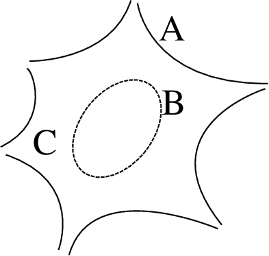
Define $\tilde{\psi}$ as the restriction of the linearising coordinates conjugating $f_{a}(z)$ to the rotation $\mathcal{R}_{\theta}$ in $\Delta_{a}$ , taking $A$ to the straight annulus $A(1,\varepsilon)$ , where $\varepsilon$ is determined by the modulus of $A$ . Also define a quasi-conformal mapping $\tilde{\phi}:A(1,\varepsilon)\to A(1,\varepsilon^{2})$ conjugating the rotation $\mathcal{R}_{\theta}$ to itself. Let $\phi$ be the composition $\tilde{\phi}\circ\tilde{\psi}$ .

Let $\mu$ be the $f_{a}$ invariant Beltrami form defined as the pull-back $\mu=\tilde{\phi}^{*}\mu_{0}$ in $A$ and spread this structure to $\cup_{n}f^{-n}_{a}(A)$ by the dynamics of $f_{a}(z)$ . Finally define $\mu=\mu_{0}$ in $\mathbb{C}\backslash\cup_{n}f^{-n}(A)$ . Observe that $\mu=\mu_{0}$ in a neighbourhood of 0. Also $\phi$ has bounded dilatation, say $k<1$ , which is also the dilatation of $\mu$ .

Now let $\mu_{t}=t\cdot\mu$ be a family of Beltrami forms with $t\in\mathbb{D}(0,1/k)$ . These new Beltrami forms are integrable, since $\|\mu_{t}\|_{\infty}=t\|\mu\|<\frac{1}{k}k=1$ . Thus by the Measurable Riemann Mapping Theorem we get an integrating map $\phi_{t}$ fixing 0,-1 and $\infty$ , such that $\phi_{t}^{*}\mu_{0}=\mu_{t}$ . Let $f^{t}=\phi_{t}\circ f_{a}\circ\phi_{t}^{-1}$ ,

Since $\mu_{t}$ is $f_{a}$ -invariant, it follows that $f^{t}(z)$ preserves the standard complex structure and hence it is holomorphic by Weyl’s lemma.

Notice also that by Theorem 2.4 in Section 2 $f^{t}(z)$ has finite order. Furthermore by the properties of the integrating map and topological considerations, it has an essential singularity at $\infty$ , a fixed point 0 with multiplier $\lambda$ and a simple critical point in -1. Finally, it has one asymptotic value $\phi_{t}(a)$ with one finite pre-image, $\phi_{t}(a-1)$ . Hence by Theorem 3.18 $f^{t}(z)=f_{a(t)}(z)$ for some $a(t)$ . Now we want to prove that $a(t)$ is analytic. First observe that for any fixed $z\in\mathbb{C}$ , the almost complex structure $\mu_{t}$ is analytic with respect to $t$ . Hence, by the MRMT, it follows that $t\mapsto\phi_{t}(z)$ is analytic with respect to $t$ . Now, $a-1$ is the finite pre-image of $v_{a}$ , so $\phi_{t}(a-1)=a(t)-1$ , and this implies $a(t)=1+\phi_{t}(a-1)$ , which implies that $a(t)$ is also analytic.

It follows that $a(t)$ is either open or constant. But $f_{a(0)}=f_{a}$ and $f_{1}$ are different mappings since the annuli $\phi_{0}(A)=A$ and $\phi_{1}(A)$ have different moduli. Then $a(t)$ is open and therefore $\{a(t),\,t\in D(0,1/k)\}$ is an open neighbourhood of $a$ which belongs to $C_{p}^{v}$ (resp. $C_{p}^{c}$ ).

If $f^{p}_{a_{0}}(v_{a_{0}})=0$ (resp. $f^{p}_{a_{0}}(-1)=0$ ), by Lemma 5 and Corollary 2 there exists an $\varepsilon>0$ such that for all $a$ close to $a_{0}$ , $\Delta_{a_{0}}\supset D(0,\varepsilon)$ . Hence a small perturbation of $f_{a_{0}}$ will still capture the orbit of $v_{a_{0}}$ (resp. -1) as we wanted.

∎

The theorem above shows that capture parameters form an open set. We call the connected components of this set, capture components, which may be asymptotic or critical depending on whether it is the asymptotic or the critical orbit which falls into $\Delta_{a}$ .

As in the case of semi-hyperbolic components, capture components are simply connected. Before showing that, we also need to prove that no critical capture component may surround $a=0$ . We just state this fact, since the proof is a reproduction of the proof of Proposition 3 above.

Proposition 6.

Let $\gamma$ be a closed curve in $W\subset C^{v}$ . Then $\mathrm{ind}(\gamma,0)=0$ .

Proposition 7.

(Theorem C, Part b) All connected components $W$ of $C^{v}$ or $C^{c}$ are simply connected.

Proof.

Let $W$ be a connected component of $C^{v}$ or $C^{c}$ and $\gamma\subset W$ a simple closed curve. Let $D$ be the bounded component of $\mathbb{C}\backslash\gamma$ . Let $U$ be a neighbourhood of $\gamma$ such that $U\subset W$ . Then, for all $a\in U$ , $f_{a}^{n}(v_{a})$ (resp. $f_{a}^{n}(-1)$ ) belongs to $\Delta_{a}$ for $n\geq n_{0}$ , and even more it remains on an invariant curve. It follows that $G_{n}^{v}(a)=f_{a}^{n}(v_{a})$ (resp. $G_{n}^{c}(a)=f_{a}^{n}(-1)$ ) is bounded in $U$ for all $n\geq n_{0}$ .

Since $G_{n}^{v}(a)$ is holomorphic in all of $\mathbb{C}$ (resp. in $\mathbb{C}^{*}$ ), we have that $G_{n}^{v}(a)$ (resp. $G_{n}^{c}(a)$ ) is holomorphic and bounded on $D$ , and hence it is a normal family in $D$ . By analytic continuation the partial limit functions must coincide, so there are no bifurcation parameters in $D$ . Hence $D\subset W$ .

∎

As it was the case with semi-hyperbolic components, it follows from Theorem 3.19 that all critical capture components must be bounded, since for $|a|$ large, the critical orbit must accumulate on $\partial\Delta_{a}$ . This proves Part c) if Theorem C. Among all asymptotic capture components, there is one that stands out in all computer drawings, precisely the main component in $C_{0}^{v}$ . That is, the set of parameters for which $v_{a}$ itself belongs to the Siegel disc.

We first observe that this component must also be bounded. Indeed, if $v_{a}\in\Delta_{a}$ then its finite pre-image $a-1$ must also be contained in the Siegel disc. But for $|a|$ large enough, the disc is contained in $D(0,R)$ , with $R$ independent of $a$ (see Theorem 3.19). Clearly $C_{0}^{v}$ has a unique component, since $v_{a}=0$ only for $a=0$ or $a=1$ . This proves Part d) of Theorem C.

The “centre” of $C_{0}^{v}$ is $a=1$ , or the map $f_{a}(z)=\lambda ze^{z}$ , for which the asymptotic value $v_{1}=0$ is the centre of the Siegel disc. This map is quite well-known, as it is, in many aspects, the transcendental analogue of the quadratic family. It is known, for example that if $\theta$ is of constant type then $\partial\Delta_{a}$ is a quasi-circle and contains the critical point. This type of properties can be extended to the whole component $C_{0}^{v}$ as shown by the following proposition.

Proposition 8.

(Proposition E, Part a) If $\theta$ is of constant type then for every $a\in C_{0}^{v}$ the boundary of the Siegel disc is a quasi-circle that contains the critical point.

Proof.

For $a=1$ , $f_{1}(z)=\lambda ze^{z}$ and we know that $\partial\Delta_{a}$ is a quasi-circle that contains the critical point (see [10]). Define $c_{n}=f_{1}^{n}(-1)$ , denote by $\mathcal{O}_{a}(-1)$ the orbit of -1 by $f_{a}(z)$ and

Then this mapping is a holomorphic motion, as it verifies

•

$H(c_{n},1)=c_{n}$ ,
•

it is injective for every $a$ , as if $v_{a}\in C_{0}^{v}$ , then $\mathcal{O}_{a}(-1)$ must accumulate on $\partial\Delta_{a}$ . Hence $f_{a}^{n}(-1)\neq f_{a}^{m}(-1)$ for all $n\neq m$ .
•

It is holomorphic with respect to $a$ for all $c_{n}$ , an obvious assertion as long as $0\notin C_{0}^{v}$ which is always true.

Now by the second $\lambda$ -lemma (Lemma 2 in Section 2), it extends quasi-conformally to the closure of $\{c_{n}\}_{n\in\mathbb{N}}$ , which contains $\partial\Delta_{a}$ . It follows that for all $a\in C_{0}^{v}$ , the boundary of $\Delta_{a}$ satisfies $\partial\Delta_{a}=H_{a}(\partial\Delta_{a})$ with $H_{a}$ quasi-conformal, and hence $\partial\Delta_{a}$ is a quasi-circle. Since $-1\in\partial\Delta_{1}$ , we have that $-1\in\partial\Delta_{a}$ .

∎

We shall see in the next section that this same argument can be generalised to other regions of parameter space.

6 Julia stability

The maps in our family are of finite type, hence $f_{a_{0}}(z)$ is $\mathcal{J}$ -stable if both sequences $\{f_{a}^{n}(-1)\}_{n\in\mathbb{Z}}$ and $\{f_{a}^{n}(v_{a})\}_{n\in\mathbb{Z}}$ are normal for $a$ in a neighbourhood of $a_{0}$ (see [16] or [7]).

We define the critical and asymptotic stable components as

	$\displaystyle\mathcal{S}^{c}$	$\displaystyle=\{a\in\mathbb{C}\|G_{n}^{c}(a)=f^{n}_{a}(-1)\text{ is normal in a neighbourhood of }a\},$
	$\displaystyle\mathcal{S}^{v}$	$\displaystyle=\{a\in\mathbb{C}\|G_{n}^{v}(a)=f^{n}_{a}(v_{a})\text{ is normal in a neighbourhood of }a\},$

respectively. Accordingly we define critical and asymptotic unstable components $\mathcal{U}^{c}$ , $\mathcal{U}^{v}$ as their complements, respectively. These stable components are by definition open, its complements closed. With this notation the set of $\mathcal{J}$ -stable parameters is then $\mathcal{S}=\mathcal{S}^{c}\cap\mathcal{S}^{v}$ .

Capture parameters and semi-hyperbolic parameters clearly belong to $\mathcal{S}^{c}$ or $\mathcal{S}^{v}$ . Next, we show that, because of the persistent Siegel disc, they actually belong to both sets.

Proposition 9.

$H^{c,v},C^{c,v}\subset\mathcal{S}$

Proof.

Suppose, say, that $a_{0}\in H^{v}$ . The orbit of $v_{a_{0}}$ tends to an attracting cycle, and hence $a_{0}\in\mathcal{S}^{v}$ . In fact, since $H^{v}$ is open, we have that $a\in\mathcal{S}^{v}$ for all $a$ in a neighbourhood $U$ of $a_{0}$ . For all these values of $a$ , the critical orbit is forced to accumulate on $\partial\Delta_{a}$ , hence $\{f_{a}^{n}(-1)\}_{n\in\mathbb{N}}$ avoids, for example, all points in $\Delta_{a}$ . It follows that $\{f_{a}^{n}(-1)\}_{n\in\mathbb{N}}$ is also normal on $U$ and therefore $a_{0}\in\mathcal{S}^{c}$ . The three remaining cases are analogous.

∎

Any other component of $\mathcal{S}$ not in $H$ or $C$ will be called a queer component, in analogy to the terminology used for the Mandelbrot set. We denote by $Q$ the set of queer components, so that $\mathcal{S}=H\cup C\cup Q$ .

At this point we want to return to the proof of Proposition 8, where we showed that, for parameters inside $C_{0}^{v}$ , the boundary of the Siegel disc was moving holomorphically with the parameter. In fact, this is a general fact for parameters in any non-queer component of the $\mathcal{J}$ -stable set.

Proposition 10.

Let $W$ be a non-queer component of $\mathcal{S}=\mathcal{S}^{c}\cap\mathcal{S}^{v}$ , and $a_{0}\in W$ . Then there exists a function $H:W\times\partial\Delta_{a_{0}}\to\partial\Delta_{a}$ which is a holomorphic motion of $\partial\Delta_{a_{0}}$ .

Proof.

Since $W$ is not queer, we have that $W\subset H\cup C$ . Let $s_{a}$ denote the singular value whose orbits accumulates on $\partial\Delta_{a}$ for $a\in W$ , so that $s_{a}\in\{-1,v_{a}\}$ . Let $s_{a}^{n}=f_{a}^{n}(s_{a})$ , and denote the orbit of $s_{a}$ by $\mathcal{O}_{a}(s_{a})$ . Then the function

is a holomorphic motion, since $\mathcal{O}_{a}(s_{a})$ must be infinite for all $n$ , and $f_{a}^{n}(s_{a})$ is holomorphic on $a$ , because $0\notin W$ . By the second $\lambda$ -lemma, $H$ extends to the closure of $\mathcal{O}_{a_{0}}(s_{a_{0}})$ which contains $\partial\Delta_{0}$ .

∎

Combined with the fact that $f_{a}(z)$ is a polynomial-like map of degree 2 for $|a|>R$ (see Theorem 3.19) we have the following immediate corollary.

Corollary 3.

(Proposition E, Part b) Let $W\subset H^{v}\cup C^{v}$ be a component intersecting $\{|z|>R\}$ where $R$ is given by Theorem 3.19 (in particular this is satisfied by any component of $H^{v}$ ). Then,

a)

if $\theta$ is of constant type, for all $a\in W$ , the boundary $\partial\Delta_{a}$ is a quasi-circle containing the critical point.
b)

Depending on $\theta\in\mathbb{R}\backslash\mathbb{Q}$ , other possibilities may occur: $\partial\Delta_{a}$ might be a quasi-circle not containing the critical point, or a $\mathscr{C}^{n},\,n\in\mathbb{N}$ Jordan curve not being a quasi-circle containing the critical point, or a $\mathscr{C}^{n},\,n\in\mathbb{N}$ Jordan curve not containing the critical point and not being a quasi-circle. In general, any possibility realised by a quadratic polynomial for some rotation number and which persists under quasi-conformal conjugacy, is realised for some $f_{a}=e^{2\pi\theta i}a(e^{z/a}(z+1-a)+a-1)$ .

Remark 7.

In general, for any $W\subset H^{v}\cup C^{v}$ we only need one parameter $a_{0}\in W$ for which one of such properties is satisfied, to have it for all $a\in W$ .

Proof of Theorem 4.22 and numerical bounds

We may suppose $\lambda\neq\pm i$ since $\theta\neq\pm 1/2$ . Let $\lambda=\lambda_{1}+i\lambda_{2}$ , $\sigma=\mathrm{Sign}\left(\lambda_{1}\right)$ and $\rho=\mathrm{Sign}\left(\lambda_{2}\right)$ . We define:

	$\displaystyle C_{1}:$	$\displaystyle=\{\sigma s+ti\|\|t\|\leq y\}$
	$\displaystyle C_{2}:$	$\displaystyle=\{\sigma t+i\rho y\|t\geq s\}$
	$\displaystyle C_{3}:$	$\displaystyle=\{\sigma t-i\rho y\|t\geq s\}$

with $y>0$ , $s>0$ , see Figure 12 for a sketch of this curves. Let $R$ be the region bounded by $C_{1}$ , $C_{2}$ , $C_{3}$ . Recall that $v_{a}=\lambda(a^{2}-a)$ is the asymptotic value. Note that we will consider $a$ real, furthermore following Figure 12, we will set $a:=-\sigma b$ with $b>0$ , as hinted by numerical experiments. Defined this way, the curves that are closer to $v_{a}$ are $C_{1}$ and $C_{2}$ . We choose $y$ and $s$ in such a way that $d(v_{a},C_{1})=d(v_{a},C_{2})$ , as in Figure 12. More precisely,

d(v_{a},C_{1,2})=|\lambda_{1}|\left(b^{2}+\sigma b\right)-s=|\lambda_{2}|(b^{2}+\sigma b)-y

and hence

y=\left(|\lambda_{1}|+|\lambda_{2}|\right)\left(b^{2}+\sigma b\right)-s.

To ease notation, define $L=\left(|\lambda_{1}|+|\lambda_{2}|\right)$ . We would like some conditions over $s$ assuring that if $b>b^{*}$ , $d(v_{a},f(\partial R))\leq d(v_{a},\partial R)$ , as this would imply $f(R)\subset R$ and thus the existence of an attracting fixed point. We write $f_{a}(z)=v_{a}+g_{a}(z)$ where $g_{a}(z)=a\cdot\lambda e^{z/a}\cdot\left(z+1-a\right)$ . Then

d(v_{a},f(\partial R))=d(0,g_{a}(\partial R))=|g_{a}(\partial R)|.

Therefore we need to find values such that the following three inequalities hold

$\displaystyle\|g_{a}(C_{1})\|$	$\displaystyle<\|\lambda_{1}\|\left(b^{2}+\sigma b\right)-s,$	(6)
$\displaystyle\|g_{a}(C_{2})\|$	$\displaystyle<\|\lambda_{1}\|\left(b^{2}+\sigma b\right)-s,$	(7)
$\displaystyle\|g_{a}(C_{3})\|$	$\displaystyle<\|\lambda_{1}\|\left(b^{2}+\sigma b\right)-s.$	(8)

For (6) to hold the following inequality needs to be satisfied

b\cdot e^{-s/b}\sqrt{\left((\sigma s+\sigma b+1)+t^{2}\right)}\stackrel{{\scriptstyle?}}{{\leq}}|\lambda_{1}|\left(b^{2}+\sigma b\right)-s.

Observe that

	$\displaystyle b\cdot e^{-s/b}\sqrt{(\sigma s+\sigma b+1)^{2}+t^{2}}$	$\displaystyle\leq b\cdot e^{-s/b}\left(\|\sigma(s+b)+1\|+y\right)=$
		$\displaystyle=b\cdot e^{-s/b}\left(s+b+\sigma+y\right)=$
		$\displaystyle=b\cdot e^{-s/b}\left(b+\sigma+L(b^{2}+\sigma b)\right),$

so we define the following function

h(s)=b\cdot e^{-s/b}\left(b+\sigma+L(b^{2}+\sigma b)\right)-|\lambda_{1}|\left(b^{2}+\sigma b\right)+s,

and we will find an argument which makes it negative. We need to find $s$ such that $h(s)<0$ and $0<s<|\lambda_{1}|(b^{2}+\sigma b)|$ . It is easy to check that $h(s)$ has a local minimum at $s^{*}:=b\log\left(b+\sigma+L(b^{2}+\sigma b)\right)$ and furthermore

h(s^{*})=b+b\log\left(b+\sigma+L(b^{2}+\sigma b)\right)-|\lambda_{1}|\left(b^{2}+\sigma b\right),

which is negative for some $b^{*}$ big enough (in Appendix 6 we will give some estimates on how big this $b^{*}$ must be as a function of $\lambda$ ). This $s^{*}$ is again in our target interval, for a big enough $b$ (note that if $h(s^{*})<0$ then $s^{*}<|\lambda_{1}|(b^{2}+\sigma b)|$ ).

From now on, let $s=s^{*}$ , and check if (7) holds, where we will put $s=s^{*}$ at the end of the calculations.

b\cdot e^{-\sigma t/\sigma b}\sqrt{\left((\sigma t+\sigma b+1)+y^{2}\right)}\stackrel{{\scriptstyle?}}{{\leq}}|\lambda_{1}|\left(b^{2}+\sigma b\right)-s.

As we have done before, expand

	$\displaystyle b\cdot e^{-\sigma t/\sigma b}\sqrt{\left((\sigma t+\sigma b+1)+y^{2}\right)}$	$\displaystyle\leq b\cdot e^{-t/b}\cdot\left(\|\sigma t+\sigma b+1\|+y\right)=$
		$\displaystyle=b\cdot e^{-t/b}\cdot\left(t+b+\sigma+y\right)=$
		$\displaystyle=b\cdot e^{-t/b}\cdot\left(t+b+\sigma+L\left(b^{2}+\sigma b\right)-s^{*}\right).$

It is easy to check that $b\cdot e^{-t/b}\cdot(b+\sigma+y)$ is a decreasing function in $t$ , and $b\cdot e^{-t/b}t$ has a local maximum at $t=b$ and is a decreasing function for $t>b$ . Then, we can bound both terms by setting $t=s^{*}$ , as $s^{*}\geq b$ whenever $b+\sigma+L(b^{2}+\sigma b)$ is bigger than $e$ , but this inequality holds if all other conditions are fulfilled. Now we must only check if

	$\displaystyle\|\lambda_{1}\|\left(b^{2}+\sigma b\right)-s^{*}$	$\displaystyle\stackrel{{\scriptstyle?}}{{\geq}}b\cdot e^{-s^{}/b}\cdot\left(s^{}+b+\sigma\|+L\left(b^{2}+\sigma b\right)-s^{*}\right)=$
		$\displaystyle=b\cdot\frac{b+\sigma+L\left(b^{2}+\sigma b\right)}{b+\sigma+L\left(b^{2}+\sigma b\right)}=b,$

which is the same inequality we have for $h(s)$ , thus it is also satisfied. Inequality (8) is equivalent to (6), hence the result follows.

Now we give numerical bounds for how big $b$ must be in Theorem 4.22. We will consider only the general case $\lambda_{1}\neq 0$ , as the other is equivalent.

Consider the inequality

b\log\left(b+\sigma+L(b^{2}+\sigma b\right))\leq-b+|\lambda_{1}|\left(b^{2}+\sigma b\right)

If this inequality holds and $b+\sigma+L(b^{2}+\sigma b)>0$ , we have the required estimates to guarantee that all required inequalities in Theorem 4.22 hold. The second inequality is clearly trivial, as it holds when $b>1$ . Now, we must find a suitable $b$ for the first.

Simplifying a $b$ factor and taking exponentials in both sides, we must check which $b$ verify

\displaystyle b+\sigma+L(b^{2}+\sigma b)\leq e^{-1+|\lambda_{1}|\sigma}e^{|\lambda_{1}|b}.

(9)

We can get a lower bound of $e^{x}$ :

\displaystyle e^{|\lambda_{1}|b}\geq 1+|\lambda_{1}|b+\frac{|\lambda_{1}|^{2}b^{2}}{2}+\frac{|\lambda_{1}|^{3}b^{3}}{6}.

And this way if

b+\sigma+L(b^{2}+\sigma b)\leq e^{-1+|\lambda_{1}|\sigma}\left(1+|\lambda_{1}|b+\frac{|\lambda_{1}|^{2}b^{2}}{2}+\frac{|\lambda_{1}|^{3}b^{3}}{6}\right),

then is also true (9). Now we must check when a degree 3 polynomial with negative dominant term has negative values. This will be true as long as $b>0$ is greater than the root with bigger modulus. It is well-known (see [13]) that a monic polynomial $z^{n}+\sum_{i}^{n-1}a_{i}z^{i}$ has its roots in a disc of radius $\max(1,\sum_{i}^{n-1}|a_{i}|)$ , so every $b>1$ and bigger than

\displaystyle\frac{6}{e^{\sigma|\lambda_{1}|-1}|\lambda_{1}|^{3}}\cdot\left(|L-e^{\sigma|\lambda_{1}|-1}\frac{|\lambda_{1}|^{2}}{2}|+|1-e^{\sigma|\lambda_{1}|-1}|\lambda_{1}|b+L\sigma b|+|b+\sigma-1|\right)

satisfies our claims.

Finer estimates for $b$ depending on $\lambda$ can be obtained with a more careful splitting of $\lambda$ space, for instance

	$\displaystyle\{\lambda\|\lambda\in S^{1}\}$	$\displaystyle=\{\lambda\in[7\pi/4,\pi/4]\}\cup\{\lambda\in[\pi/4,3\pi/4]\}\cup\{\lambda\in[3\pi/4,5\pi/4]\}$
		$\displaystyle\cup\{\lambda\in[5\pi/4,7\pi/4]\}=B_{1}\cup B_{2}\cup B_{3}\cup B_{4}.$

The proof can be adapted with very minor changes to this partition, although the exposition and calculations are more cumbersome.

Acknowledgements

The authors wish to thank Xavier Buff and Lasse Rempe for helpful conversations. Both authors were partially supported by Spanish grant MICINN MTM2006-05849/Consolider and European funds MCRTN-CT-2006-035651. The second author was also partially supported by Spanish grant MICINN MTM2008-01486 and by Catalan grant CIRIT 2005/SGR01028.

References

[1] Lars V. Ahlfors. Lectures on quasiconformal mappings, volume 38 of University Lecture Series. American Mathematical Society, Providence, RI, second edition, 2006. With supplemental chapters by C. J. Earle, I. Kra, M. Shishikura and J. H. Hubbard.
[2] I. N. Baker and P. J. Rippon. Iteration of exponential functions. Annales Academiae Scientiarum Fennicae Series A I Mathematica, 9:49–77, 1984.
[3] Clara Bodelón, Robert L. Devaney, Michael Hayes, Gareth Roberts, Lisa R. Goldberg, and John H. Hubbard. Hairs for the complex exponential family. International Journal of Bifurcation and Chaos in Applied Sciences and Engineering, 9(8):1517–1534, 1999.
[4] Bodil Branner and Núria Fagella. Quasiconformal surgery in holomorphic dynamics. Work in progress.
[5] John B. Conway. Functions of one complex variable, volume 11 of Graduate Texts in Mathematics. Springer-Verlag, New York, second edition, 1978.
[6] Adrien Douady. Disques de Siegel et anneaux de Herman. Astérisque, (152-153):4, 151–172 (1988), 1987. Séminaire Bourbaki, Vol. 1986/87.
[7] A. È. Erëmenko and M. Yu. Lyubich. Dynamical properties of some classes of entire functions. Annales de l’Institut Fourier. Université de Grenoble, 42(4):989–1020, 1992.
[8] Núria Fagella. Limiting dynamics for the complex standard family. International Journal of Bifurcations and Chaos in Applied Sciences and Engineering, 5(3):673–699, 1995.
[9] Núria Fagella, Tere M. Seara, and Jordi Villanueva. Asymptotic size of Herman rings of the complex standard family by quantitative quasiconformal surgery. Ergodic Theory and Dynamical Systems, 24(3):735–766, 2004.
[10] Lukas Geyer. Siegel discs, Herman rings and the Arnold family. Transactions of the American Mathematical Society, 353(9):3661–3683 (electronic), 2001.
[11] Lisa R. Goldberg and Linda Keen. A finiteness theorem for a dynamical class of entire functions. Ergodic Theory and Dynamical Systems, 6(2):183–192, 1986.
[12] Michael-R. Herman. Are there critical points on the boundaries of singular domains? Communications in Mathematical Physics, 99(4):593–612, 1985.
[13] Holly P. Hirst and Wade T. Macey. Bounding the roots of polynomials. The College Mathematics Journal, 28(4):292–295, Sept 1997.
[14] R. Mañé, P. Sad, and D. Sullivan. On the dynamics of rational maps. Annales Scientifiques de l’École Normale Supérieure (4), 16(2):193–217, 1983.
[15] Ricardo Mañé. On a theorem of Fatou. Boletim de Sociedade Brasileira de Matemática (N.S.), 24(1):1–11, 1993.
[16] Curtis T. McMullen. Complex dynamics and renormalization, volume 135 of Annals of Mathematics Studies. Princeton University Press, Princeton, NJ, 1994.
[17] John Milnor. Dynamics in one complex variable, volume 160 of Annals of Mathematics Studies. Princeton University Press, Princeton, NJ, third edition, 2006.
[18] Ricardo Pérez-Marco. Fixed points and circle maps. Acta Mathematica, 179(2):243–294, 1997.
[19] Lasse Rempe. On a question of Herman, Baker and Rippon concerning Siegel disks. Bulletin of the London Mathematical Society, 36(4):516–518, 2004.
[20] Lasse Rempe. Siegel disks and periodic rays of entire functions. Journal für die reine und angewandte Mathematik, 624:81–102, 2008.
[21] James T. Rogers, Jr. Singularities in the boundaries of local Siegel disks. Ergodic Theory and Dynamical Systems, 12(4):803–821, 1992.
[22] James T. Rogers, Jr. Recent results on the boundaries of Siegel disks. In Progress in holomorphic dynamics, volume 387 of Pitman Research Notes in Mathematical Series, pages 41–49. Longman, Harlow, 1998.
[23] Gunther Rottenfusser. Dynamical fine structure of entire transcendental functions. Doctoral Thesis, International University Bremen, 2005.
[24] Carl Ludwig Siegel. Iteration of analytic functions. Annals of Mathematics (2), 43:607–612, 1942.
[25] Zbigniew Slodkowski. Holomorphic motions and polynomial hulls. Proceedings of the American Mathematical Society, 111(2):347–355, 1991.
[26] Jean-Christophe Yoccoz. Petits diviseurs en Dimension 1. Number 231 in Astérisque. Société Mathématique de France, 1995.
[27] Jean-Christophe Yoccoz. Analytic linearization of circle diffeomorphisms. In Dynamical systems and small divisors (Cetraro, 1998), volume 1784 of Lecture Notes in Mathematics, pages 125–173. Springer, Berlin, 2002.
[28] Saeed Zakeri. Dynamics of cubic Siegel polynomials. Communications in Mathematical Physics, 206(1):185–233, 1999.

$\displaystyle\|g_{a}(C_{1})\|$	$\displaystyle<\|\lambda_{1}\|\left(b^{2}+\sigma b\right)-s,$	(6)
$\displaystyle\|g_{a}(C_{2})\|$	$\displaystyle<\|\lambda_{1}\|\left(b^{2}+\sigma b\right)-s,$	(7)
$\displaystyle\|g_{a}(C_{3})\|$	$\displaystyle<\|\lambda_{1}\|\left(b^{2}+\sigma b\right)-s.$	(8)

An entire transcendental family with a persistent Siegel disc

Abstract

1 Introduction

Theorem A.

Theorem B.

Theorem C.

Proposition 1.

Proposition 2.

2 Preliminary results

2.1 Quasi-conformal mappings and holomorphic motions

Definition 1.

Definition 2.

Theorem 2.4 ([9, p. 750]).

Theorem 2.5 ((Measurable Riemann Mapping, MRMT)).

Theorem 2.6 ((MRMT with dependence of parameters)).

Definition 3.

Lemma 1 ((First λ\lambda-lemma)).

Lemma 2 ((Second λ\lambda-lemma)).

2.2 Hadamard’s factorisation theorem

Definition 4.

Definition 5.

Definition 6.

Theorem 2.7.

Theorem 2.8 ((Hadamard’s factorisation)).

2.3 Siegel discs

Theorem 2.9 ((Brjuno-Rüssmann)).

Definition 7.

Theorem 2.10.

Theorem 2.11 ((Douady-Ghys)).

Theorem 2.12 ((Herman)).

Definition 8.

Theorem 2.13 ((Rempe), [19]).

2.4 Topological results

Definition 9.

Definition 10.

Definition 11.

Theorem 2.14.

Theorem 2.15.

Proof.

Theorem 2.16 ((Vietoris-Begle)).

Theorem 2.17 ((Alexander’s duality)).

Remark 1.

Definition 12.

Definition 13.

Remark 2.

Remark 3.

Proof of Theorem 2.14.

3 The (entire transcendental) family faf_{a}

Theorem 3.18.

Proof.

3.1 Dynamical planes

Theorem 3.19.

Corollary 1.

Theorem 3.20.

Proof.

Proof of Part a).

Proof of part b).

Remark 4.

3.2 Large values of |a||a|: Proof of theorem 3.19

Remark 5.

4 Semi-hyperbolic components: Proof of Theorem B

Proposition 3.

Proof.

Lemma 3.

Proof.

Proposition 4.

Proof.

Lemma 4.

Proof.

Theorem 4.21.

Proof.

Theorem 4.22.

Proof.

Remark 6.

4.1 Parametrisation of HpvH_{p}^{v}: Proof of Theorem B, Part b

Theorem 4.23.

Proof.

4.2 Parametrisation of HpcH_{p}^{c}: Proof of Theorem B, Part d

Proposition 5.

Proof.

Lemma 1 ((First $\lambda$ -lemma)).

Lemma 2 ((Second $\lambda$ -lemma)).

3 The (entire transcendental) family $f_{a}$

3.2 Large values of $|a|$ : Proof of theorem 3.19

4.1 Parametrisation of $H_{p}^{v}$ : Proof of Theorem B, Part b

4.2 Parametrisation of $H_{p}^{c}$ : Proof of Theorem B, Part d