The Top Triangle Moose: Combining Higgsless and Topcolor Mechanisms for Mass Generation

Preprint: MSUHEP-090630

R. Sekhar Chivukula Email: sekhar@msu.edu Affiliation: Department of Physics and Astronomy,
Michigan State University,
East Lansing, Michigan 48824, USA Neil D. Christensen Email: neil@pa.msu.edu Affiliation: Department of Physics and Astronomy,
Michigan State University,
East Lansing, Michigan 48824, USA Baradhwaj Coleppa Email: baradhwaj@pa.msu.edu Affiliation: Department of Physics and Astronomy,
Michigan State University,
East Lansing, Michigan 48824, USA Elizabeth H. Simmons Email: esimmons@msu.edu Affiliation: Department of Physics and Astronomy,
Michigan State University,
East Lansing, Michigan 48824, USA

August 24, 2026

Abstract

We present the details of a deconstructed model that incorporates both Higgsless and top-color mechanisms. The model alleviates the tension between obtaining the correct top quark mass and keeping $\Delta\rho$ small that exists in many Higgsless models. It does so by singling out the top quark mass generation as arising from a Yukawa coupling to an effective top-Higgs which develops a small vacuum expectation value, while electroweak symmetry breaking results largely from a Higgsless mechanism. As a result, the heavy partners of the SM fermions can be light enough to be seen at the LHC. After presenting the model, we detail the phenomenology, showing that for a broad range of masses, these heavy fermions are discoverable at the LHC.

I Introduction

Understanding the mechanism of electroweak symmetry breaking (EWSB) is one of the most exciting problems facing particle physics today. The Standard Model (SM), though phenomenologically successful, relies crucially on the existence of a scalar particle, the Higgs boson [1], which has not been discovered in collider experiments. Over the last few years, Higgsless models [2] have emerged as a novel way of understanding the mechanism of EWSB without the presence of a scalar particle in the spectrum. In an extra dimensional context, these can be understood in terms of a $SU(2)\times SU(2)\times U(1)$ gauge theory in the bulk of a finite $AdS$ spacetime [4, 6, 5, 3], with symmetry breaking encoded in the boundary conditions of the gauge fields. These models can be thought of as dual to technicolor models, in the language of the AdS/CFT correspondence [7, 8, 9, 10]. One can understand the low energy properties of such theories in a purely four dimensional picture by invoking the idea of deconstruction [11, 12]. The “bulk” of the extra dimension is then replaced by a chain of gauge groups strung together by non linear sigma model fields. The spectrum typically includes extra sets of charged and neutral vector bosons and heavy fermions. The unitarization of longitudinal $W$ boson scattering is accomplished by diagrams involving the exchange of the heavy gauge bosons [13, 14, 15, 16], instead of a Higgs. A general analysis of Higgsless models [17, 18, 19, 20, 21, 22] suggests that to satisfy the requirements of precision electroweak constraints, the SM fermions have to be ‘delocalized’ into the bulk. The particular kind of delocalization that helps satisfy the precision electroweak constraints, “ideal fermion delocalization’” [23], dictates that the light fermions be delocalized in such a way that they do not couple to the heavy charged gauge bosons. The simplest framework that captures all these ideas, a three site Higgsless model, is presented in [24], where there is just one gauge group in the bulk and correspondingly, only one set of heavy vector bosons. It was shown that the twin constraints of getting the correct value of the top quark mass and having an admissible $\rho$ parameter necessarily push the heavy fermion masses into the TeV regime [24] in that model.

In this paper, we seek to decouple these constraints by combining the Higgsless mechanism with aspects of topcolor [25, 26]. The goal is to separate the bulk of electroweak symmetry breaking from third family mass generation. In this way, one can obtain a massive top quark and heavy fermions in the sub TeV region, without altering tree level electroweak predictions. In an attempt to present a minimal model with these features, we modify the three site model by adding a “top Higgs” field, $\Phi,$ that couples preferentially to the top quark. The resulting model is shown in Moose notation [27] in Figure 1; we will refer to it as the “top triangle moose” to distinguish it from other three-site ring models in the literature in which all of the links are non-linear sigmal models, such as the ring model explored in [28] or BESS [29, 30] and hidden local symmetry [31, 32, 33, 34, 35] theories.

The idea of a top Higgs is motivated by top condensation models, ranging from the top mode standard model [36, 37, 38, 39, 40, 41] to topcolor assisted technicolor[43, 44, 42, 45, 46], to the top quark seesaw [47, 48] to bosonic topcolor [49, 50]. The specific framework constructed here is most closely aligned with topcolor assisted technicolor theories [43, 44, 42, 45, 46] in which EWSB occurs via technicolor interactions while the top mass has a dynamical component arising from topcolor interactions and a small component generated by an extended technicolor mechanism. The dynamical bound state arising from topcolor dynamics can be identified as a composite top Higgs field, and the low-energy spectrum includes a top Higgs boson. The extra link in our triangle moose that corresponds to the top Higgs field results in the presence of uneaten Goldstone bosons, the top pions, which couple preferentially to the third generation. The model can thus be thought of as the deconstructed version of a topcolor assisted technicolor model.

We start by presenting the model in section II, and describing the electroweak sector. The gauge sector is the same as in BESS [29, 30] or hidden local symmetry [31, 32, 33, 34, 35] theories, while the fermion sector is generalized from that of the three site model [24] and the symmetry-breaking sector resembles that of topcolor-assisted technicolor [43, 44, 42, 45, 46]. In section III, we compute the masses and wave functions of the gauge bosons and describe the limits in which we work. We then move on to consider the fermionic sector in section IV. Here, we also explain how the ideal delocalization condition works for the light fermions. In section V, we compute the couplings of the fermions to the charged and neutral gauge bosons. In section VI, the top quark sector is presented. After calculating the mass of the top quark, we describe how the top quark is delocalized in this model by looking at the tree level value of the $Zb\bar{b}$ coupling. In section VII, we carry out the detailed collider phenomenology of the heavy $U,D,C$ and $S$ quarks. After comparing our phenomenological analysis with others in the literature in section VIII, we present our conclusions in section IX.

II The Model

Before we present the details of our model, we recall the essential features of the closely related three site model that [24] pertain to the heavy fermion mass. The three site model is a maximally deconstructed version of a Higgsless extra dimensional model, with only one extra $SU(2)$ gauge group, as compared to the SM. Thus, there are three extra gauge bosons, which contribute to unitarizing the $W_{L}W_{L}$ scattering in place of a Higgs. The LHC phenomenology of these extra vector bosons is discussed in [51, 52]. Also incorporated in the three site model is a heavy Dirac partner for every SM fermion. The presence of these new fermions, in particular, the heavy top and bottom quarks, gives rise to new one-loop contributions to $\Delta\rho$ , where $\rho$ is the ratio of the strengths of the low energy isotriplet neutral and charged current interactions. Precision measurements require $\Delta\rho$ to be $<\mathcal{O}(10^{-3})$ and this constraint, along with the need to obtain the large top quark mass, pushes the heavy quark mass into the multi TeV range, too high to be seen at the LHC. We seek to reduce this tension by separating the top quark mass generation from the rest of electroweak symmetry breaking in this model, an approach motivated by top-color scenarios.

The electroweak gauge structure of our model is $SU(2)_{0}\times SU(2)_{1}\times U(1)_{2}$ . This is shown using Moose notation [27] in Figure 1, in which the $SU(2)$ groups are associated with sites 0 and 1, and the $U(1)$ group is associated with site 2.¹¹ 1 Note that $U(1)_{2}$ is embedded as a gauged $\tau^{3}$ of $SU(2)$ – see Eqn. (13) below. The SM fermions deriving their $SU(2)$ charges mostly from site 0 (which is most closely associated with the SM $SU(2)$ ) and the bulk fermions mostly from site 1. The extended electroweak gauge structure of the theory is the same as that of the BESS models [29, 30], motivated by models of hidden local symmetry (with $a\neq 1$ ) [31, 32, 33, 34, 35].

Refer to caption — Figure 1: The $SU(2)\times SU(2)\times U(1)$ gauge structure of the model in Moose notation [27]. The $SU(2)$ coupling $g$ and $U(1)$ coupling $g^{\prime}$ of sites 0 and 2 are approximately the SM $SU(2)$ and hypercharge gauge couplings, while the $SU(2)$ coupling $\tilde{g}$ represents the ’bulk’ gauge coupling. The left (right) handed light fermions are mostly localized at site 0 (2) while their heavy counterparts are mostly at site 1. The links connecting sites 0 and 1 and sites 1 and 2 are non linear sigma model fields while the one connecting sites 0 and 2 is a linear sigma field.

The non linear sigma field $\Sigma_{01}$ is responsible for breaking the $SU(2)_{0}\times SU(2)_{1}$ gauge symmetry down to $SU(2)$ , and field $\Sigma_{12}$ is responsible for breaking $SU(2)_{1}\times U(1)_{2}$ down to $U(1)$ . The left handed fermions are $SU(2)$ doublets residing at sites 0 ( $\psi_{L0}$ ) and 1 ( $\psi_{L1}$ ), while the right handed fermions are a doublet under $SU(2)_{1}$ ( $\psi_{R1}$ ) and two $SU(2)$ -singlet fermions at site 2 ( $u_{R2}$ and $d_{R2}$ ). The fermions $\psi_{L0}$ , $\psi_{L1}$ , and $\psi_{R1}$ have $U(1)$ charges ( $Y$ ) typical of the left-handed $SU(2)$ doublets in the SM, $+1/6$ for quarks and $-1/2$ for leptons. Similarly, the fermion $u_{R2}$ has a $U(1)$ charge typical for the right-handed up-quarks ( $+2/3$ ) and $d_{R2}$ has the $U(1)$ charge typical for the right-handed down-quarks ( $-1/3$ ); the right-handed leptons would, likewise, have $U(1)$ charges corresponding to their SM hypercharge values. Also, the the third component of isospin, $T_{3}$ , takes values $+1/2$ for “up” type fermions and $-1/2$ for “down” type fermions, just like in the SM. The electric charge assignment follows the relation $Q=T_{3}+Y$ . The fermion charge assignments of the quarks are summarized in Table 1; leptons follow a similar pattern.

	$\psi_{L0}$ ,	$\psi_{L1}$ , $\psi_{R1}$	$u_{R2}$ , $d_{R2}$
$SU(2)_{0}$	2	1	1
$SU(2)_{1}$	1	2	1
$U(1)_{2}$	$\frac{1}{6}$	$\frac{1}{6}$	$\frac{2}{3}$ or $-\frac{1}{3}$

Table 1: Electroweak charge assignments of the quarks. Leptons follow a similar pattern.

We add a ‘top-Higgs’ link to separate the top quark mass generation from the rest of electroweak symmetry breaking. To this end, we let the top quark couple preferentially to the top Higgs link via the Largangian:

\mathcal{L}_{top}=-\lambda_{t}\bar{\psi}_{L0}\,\Phi\,t_{R}+h.c.

(1)

The top Higgs field is described by the Lagrangian:

\mathcal{L}_{\Phi}=\frac{1}{2}D_{\mu}\Phi^{\dagger}D_{\mu}\Phi-V(\Phi),

(2)

where the potential $V(\Phi)$ is minimized at $\left<\Phi\right>=f$ . When the field $\Phi$ develops a non zero vacuum expectation value, Eqn.(1) generates a top quark mass term. Since we want most electroweak symmetry breaking to come from the Higgsless side, we choose the vacuum expectation value associated with the non linear sigmal model fields to be $F=\sqrt{2}\,v$ $\textrm{cos}\,\omega$ (for simplicity, we choose the vev of both the non linear sigma model fields to be the same) and the one associated with the top Higgs sector to be $f=\langle\Phi\rangle=v$ $\textrm{sin\,}\omega$ (where $\omega$ is a small parameter). The top Higgs sector also includes the uneaten Goldstone bosons, the top pions. The interactions of these top pions can be derived from Eqn.(2) by writing the top Higgs field in the form:

\Phi=\left(\begin{array}[]{c}(f+H+i\pi^{0})/\sqrt{2}\\ i\pi^{-}\end{array}\right),

(3)

where $f$ is defined above and $H$ is the top Higgs. The Extended Technicolor [54, 53] induced “plaquette” terms that align the technicolor vacuum with the topcolor vacuum and give mass to the top pions can be written as:

\mathcal{L}_{\pi}=4\pi\kappa v^{3}\textrm{Tr}\left({\cal M}\Sigma_{01}\Sigma_{12}^{\dagger}\right),

(4)

where $\kappa$ is a dimensionless parameter and ${\cal M}=(i\sigma^{2}\Phi^{*}\ \Phi)$ is the Higgs field in $2\times 2$ matrix form. In this paper we restrict our attention to the phenomenology of the fermion and gauge sectors and, therefore, here we assume that the top-pions are sufficiently heavy so as not to affect electroweak phenomenology. The phenomenology of the top pion sector will be considered in a future publication.

The mass terms for the light fermions arise from Yukawa couplings of the fermionic fields with the non linear sigma fields

\displaystyle\mathcal{L}

\displaystyle=

\displaystyle M_{D}\left[\epsilon_{L}\bar{\psi}_{L0}\Sigma_{01}\psi_{R1}+\bar{\psi}_{R1}\psi_{L1}+\bar{\psi}_{L1}\Sigma_{12}\left(\begin{array}[]{cc}\epsilon_{uR}&0\\ 0&\epsilon_{dR}\end{array}\right)\left(\begin{array}[]{c}u_{R2}\\ d_{R2}\end{array}\right)\right].

We have denoted the Dirac mass (that sets the scale of the heavy fermion mass) as $M_{D}$ . Here, $\epsilon_{L}$ is a parameter that describes the degree of delocalization of the left handed fermions and is flavor universal. All the flavor violation for the light fermions is encoded in the last term; the delocalization parameters for the right handed fermions, $\epsilon_{fR}$ , can be adjusted to realize the masses and mixings of the up and down type fermions.²² 2 The model has “next to minimal” flavor violation [55]. For our phenomenological study, we will, for the most part, assume that all the fermions, except the top, are massless and hence will set these $\epsilon_{fR}$ parameters to zero. We will see in Section VI C that even $\epsilon_{tR}$ is small, since the top quark’s mass is dominated by the top Higgs contribution (see Eqn.(1)). Therefore, the top quark mass does not severely constrain $\Delta\rho$ , and correspondingly, there will be none of the tension between the heavy quark mass, $M_{D}$ , and one loop contributions to $\Delta\rho$ , that exists in the three site model. This enables us to have heavy quarks in this model that are light enough to be discovered at the LHC - we will investigate their phenomenology in Section VII.

III Masses and Eigenstates

In addition to the SM $\gamma$ , $Z$ and $W$ bosons, we also have the heavy partners, $W^{\prime}$ and $Z^{\prime}$ because of the extra $SU(2)$ group. The canonically normalized kinetic energy terms of the gauge fields can be written down in the usual way:

\mathcal{L}_{KE}=-\frac{1}{4}F^{a}_{0\mu\nu}F_{0}^{a\mu\nu}-\frac{1}{4}F^{b}_{1\mu\nu}F_{1}^{b\mu\nu}-\frac{1}{4}B_{\mu\nu}B^{\mu\nu}.

(10)

In this section, we review the masses and wave functions of the gauge bosons, which are the same as those in the BESS model [29, 30].

The masses of the gauge bosons come from the usual sigma model Lagrangian:

\mathcal{L}_{gauge}=\frac{F^{2}}{4}\textrm{Tr}[D_{\mu}\Sigma_{01}^{\dagger}D_{\mu}\Sigma_{01}]+\frac{F^{2}}{4}\textrm{Tr}[D_{\mu}\Sigma_{12}^{\dagger}D_{\mu}\Sigma_{12}]+\frac{1}{2}[D_{\mu}\Phi^{\dagger}D_{\mu}\Phi],

(11)

where the covariant derivatives are:

$\displaystyle D_{\mu}\Sigma_{01}$	$\displaystyle=\partial_{\mu}\Sigma_{01}+igW_{0\mu}\Sigma_{01}-i\tilde{g}\Sigma_{01}W_{1\mu}$	(12)
$\displaystyle D_{\mu}\Sigma_{12}$	$\displaystyle=\partial_{\mu}\Sigma_{12}+i\tilde{g}W_{1\mu}\Sigma_{12}-ig^{\prime}\Sigma_{12}\,\tau^{3}\,B_{2\mu},$	(13)
$\displaystyle D_{\mu}\Phi$	$\displaystyle=\partial_{\mu}\Phi+igW_{0\mu}\Phi-\frac{ig^{\prime}}{2}B_{2\mu}\Phi~,$	(14)

$W_{0\mu}\equiv W_{0\mu}^{a}\tau^{a},\,W_{1\mu}\equiv W_{1\mu}^{a}\tau^{a}$ (where $\tau^{a}=\sigma^{a}/2$ are $SU(2)$ generators), and $\Sigma_{01}$ and $\Sigma_{12}$ are 2 $\times$ 2 hermitian matrix fields. We will parametrize the gauge couplings in the following form:

g_{0}=\frac{e}{\textrm{sin}\,\theta\,\textrm{cos\,}\phi}\,\,\,\,\,\tilde{g}=\frac{e}{\textrm{sin}\,\theta\,\textrm{sin\,}\phi}\,\,\,\,\,g^{\prime}=\frac{e}{\textrm{cos}\,\theta}.

(15)

We will find the mass eigenvalues and eigenvectors perturbatively in the small parameter $\sin\phi$ , which we will call $x$ .

From the above Lagrangian, one can get the mass matrix for the gauge bosons by working in the unitary gauge ( $\Sigma_{01}=\Sigma_{12}=1$ ) and collecting the coefficients of the terms quadratic in the gauge fields.

The charged gauge boson mass matrix is thus given by:

M_{W}^{2}=\frac{e^{2}\,v^{2}}{4\,x^{2}\,\textrm{sin}^{2}\,\theta}\,\left(\begin{array}[]{cc}\frac{x^{2}}{1-x^{2}}(1+\textrm{cos}^{2}\,\omega)&-\frac{2x}{\sqrt{1-x^{2}}}\textrm{cos}^{2}\,\omega\\ -\frac{2x}{\sqrt{1-x^{2}}}\textrm{cos}^{2}\,\omega&4\,\textrm{cos}^{2}\omega\end{array}\right).

(16)

This matrix can be diagonalized perturbatively in $x$ . We find the light $W$ has the following mass and eigenvector (note that the above formulae are valid to corrections of $\mathcal{O}(x^{3})$ , as are all the other eigenvalues and couplings in this paper):

M_{W}^{2}=\frac{e^{2}v^{2}}{4\,\textrm{sin}^{2}\,\theta}\left(1+\frac{3x^{2}}{4}\right)

(17)

W^{\mu}=v_{w}^{0}W_{0}^{\mu}+v_{w}^{1}W_{1}^{\mu}=\left(1-\frac{x^{2}}{8}\right)W_{0}^{\mu}+\frac{1}{2}xW_{1}^{\mu}.

(18)

Here, $W_{0}$ and $W_{1}$ are the gauge bosons associated with sites 0 and 1. Since $x$ is small, we note that the light $W$ resides primarily at site 0. The heavy $W$ eigenvector is orthogonal to the above and has a mass:

M_{W^{\prime}}^{2}=\frac{e^{2}\,v^{2}\textrm{cos}^{2}\,\omega}{4\,\textrm{sin}^{2}\,\theta\,x^{2}}\left(4+x^{2}\right).

(19)

To leading order, the relation between the light and heavy charged gauge boson masses is

\frac{M_{W}^{2}}{M_{W^{\prime}}^{2}}=\frac{x^{2}}{4\,\textrm{cos}^{2}\,\omega}.

(20)

The neutral gauge bosons’ mass matrix is given by:

\displaystyle M_{Z}^{2}=\frac{e^{2}\,v^{2}}{4\,x^{2}\,\textrm{sin}^{2}\,\theta}\left(\begin{array}[]{ccc}\frac{x^{2}}{1-x^{2}}(1+\textrm{cos}^{2}\,\omega)&-\frac{2x}{\sqrt{1-x^{2}}}\textrm{cos}^{2}\,\omega&-\frac{x^{2}}{\sqrt{1-x^{2}}}\textrm{sin}^{2}\omega\,\textrm{tan}\,\theta\\ -\frac{2x}{\sqrt{1-x^{2}}}\textrm{cos}^{2}\,\omega&4\,\textrm{cos}^{2}\omega&-2\,x\textrm{\, cos}^{2}\,\omega\textrm{\, tan}\,\theta\\ -\frac{x^{2}}{\sqrt{1-x^{2}}}\textrm{sin}^{2}\omega\,\textrm{tan}\,\theta&-2\,x\,\textrm{cos}^{2}\,\omega\,\textrm{tan}\,\theta&x^{2}(1+\textrm{cos}^{2}\,\omega)\textrm{tan}^{2}\,\theta\end{array}\right).

This mass matrix has a zero eigenvalue (the photon), the eigenvector of which may be written exactly as:

A^{\mu}=\frac{e}{g}W_{0}^{\mu}+\frac{e}{\tilde{g}}W_{1}^{\mu}+\frac{e}{g^{\prime}}B^{\mu}.

(25)

Requring that this state be properly normalized, we get the relation between the couplings implied by Eqn. (15):

\frac{1}{e^{2}}=\frac{1}{g^{2}}+\frac{1}{\tilde{g}^{2}}+\frac{1}{g^{\prime 2}}.

(26)

The light $Z$ boson has the mass

M_{Z}^{2}=\frac{e^{2}\,v^{2}}{4\,\textrm{sin}^{2}\,\theta\,\textrm{ cos}^{2}\,\theta}\left(1+x^{2}\left(1-\frac{\textrm{sec}^{2}\,\theta}{4}\right)\right),

(27)

and the corresponding eigenvector

Z^{\mu}=v_{z}^{0}W_{0}^{\mu}+v_{z}^{1}W_{1}^{\mu}+v_{z}^{2}B^{\mu},

(28)

where

v_{z}^{0}=\frac{1}{8}\,(4(-2+x^{2})\textrm{cos\,}\theta-3\,x^{2}\textrm{sec}\,\theta),\,\,\,\,v_{z}^{1}=\frac{1}{2}\,x(-2\textrm{cos}^{2}\,\theta+1)\textrm{sec}\,\theta,\,\,\,\,\,\,v_{z}^{2}=\textrm{sin}\,\theta-\frac{1}{2}x^{2}\,\textrm{sec}\,\theta\,\textrm{tan}\,\theta.

The heavy neutral vector boson, which we call $Z^{\prime}$ , has a mass and eigenvector

M_{Z^{\prime}}^{2}=\frac{e^{2}\,v^{2}\,\textrm{cos}^{2}\,\omega}{4\,\textrm{sin}^{2}\,\theta\,x^{2}}\left(4+x^{2}\textrm{sec}^{2}\,\theta\right)

(29)

Z^{\prime\mu}=v_{z^{\prime}}^{0}W_{0}^{\mu}+v_{z^{\prime}}^{1}W_{1}^{\mu}+v_{z^{\prime}}^{2}B^{\mu},

(30)

where

v_{z^{\prime}}^{0}=\frac{1}{2}\,x,\,\,\,\,v_{z^{\prime}}^{1}=-1+\frac{1}{8}\,x^{2}\,\textrm{sec}^{2}\,\theta,\,\,\textrm{and}\,\,\,\,v_{z^{\prime}}^{2}=\frac{1}{2}\,x\textrm{\, tan}\,\theta.

For small $x$ , it is seen that the $Z^{\prime}$ is mainly located at site 1, while the $Z$ is concentrated at sites 0 and 2, as one would expect.

IV Fermion wave functions and Ideal delocalization

In this section, we will review the masses and wave functions of the light fermions and their heavy partners. We will then discuss how to “ideally delocalize” the light fermions, which will make the tree level value of the $S$ parameter vanish [23].

IV.1 Masses and wave functions

Working in the unitary gauge ( $\Sigma_{01}=\Sigma_{12}=1),$ the mass matrices of the light quarks and their heavy partners can be derived from Eqn. (II) and take the form:

\displaystyle M_{u,d}=M_{D}\left(\begin{array}[]{cc}\epsilon_{L}&0\\ 1&\epsilon_{uR,dR}\end{array}\right).

The subscripts $u(d)$ denote up (down) quarks and $M_{D}$ is the Dirac mass, introduced in Eqn. (II). Diagonalizing the matrix perturbatively in $\epsilon_{L}$ , we find the light eigenvalue:

m_{f}=\frac{M_{D}\epsilon_{L}\epsilon_{fR}}{\sqrt{1+\epsilon_{fR}^{2}}}\left[1-\frac{\epsilon_{L}^{2}}{2(1+\epsilon_{fR}^{2})}+...\right].

(34)

Note that $m_{f}$ is proportional to the flavor-specific parameter $\epsilon_{fR}$ , where $f$ is any light SM fermion (except the top). The heavy Dirac quark has a mass:

m_{F}=M_{D}\sqrt{1+\epsilon_{fR}^{2}}\left[1+\frac{\epsilon_{L}^{2}}{2(1+\epsilon_{fR}^{2})^{2}}+....\right].

(35)

The left and right handed eigenvectors of the light up quarks are

\displaystyle u_{L}

\displaystyle=

\displaystyle u_{L}^{0}\psi_{L0}+u_{L}^{1}\psi_{L1}=\left(-1+\frac{\epsilon_{L}^{2}}{2(1+\epsilon_{uR}^{2})^{2}}\right)\psi_{L0}+\left(\frac{\epsilon_{L}}{1+\epsilon_{uR}^{2}}\right)\psi_{L1}

(36)

\displaystyle u_{R}

\displaystyle=

\displaystyle u_{R}^{1}\psi_{R1}+u_{R}^{2}u_{R2}=\left(-\frac{\epsilon_{uR}}{\sqrt{1+\epsilon_{uR}^{2}}}+\frac{\epsilon_{L}^{2}\epsilon_{uR}}{(1+\epsilon_{uR}^{2})^{5/2}}\right)\psi_{R1}+\left(\frac{1}{\sqrt{1+\epsilon_{uR}^{2}}}+\frac{\epsilon_{L}^{2}\epsilon_{uR}^{2}}{(1+\epsilon_{uR}^{2})^{5/2}}\right)u_{R2}.

(37)

The left and right handed eigenvectors of the heavy partners (denoted by $U_{L,R}$ ) are orthogonal to Eqn.(36) and Eqn.(37):

\displaystyle U_{L}

\displaystyle=

\displaystyle U_{L}^{0}\psi_{L0}+U_{L}^{1}\psi_{L1}=\left(-\frac{\epsilon_{L}}{1+\epsilon_{uR}^{2}}\right)\psi_{L0}+\left(-1+\frac{\epsilon_{L}^{2}}{2(1+\epsilon_{uR}^{2})^{2}}\right)\psi_{L1}

(38)

\displaystyle U_{R}

\displaystyle=

\displaystyle U_{R}^{1}\psi_{R1}+U_{R}^{2}u_{R2}=\left(-\frac{1}{\sqrt{1+\epsilon_{uR}^{2}}}-\frac{\epsilon_{L}^{2}\epsilon_{uR}^{2}}{(1+\epsilon_{uR}^{2})^{5/2}}\right)\psi_{R1}+\left(-\frac{\epsilon_{uR}}{\sqrt{1+\epsilon_{uR}^{2}}}+\frac{\epsilon_{L}^{2}\epsilon_{uR}}{(1+\epsilon_{uR}^{2})^{5/2}}\right)u_{R2}.

(39)

The eigenvectors of other fermions can be obtained by the replacement $\epsilon_{uR}\rightarrow\epsilon_{fR}$ .

IV.2 Ideal fermion delocalization

The tree level contributions to precision measurements in Higgsless models come from the coupling of standard model fermions to the heavy gauge bosons and deviations in SM couplings. It was shown in [23] that it is possible to delocalize the light fermions in such a way that they do not couple to these heavy bosons and thus minimize the deviations in precision electroweak parameters. The coupling of the heavy $W^{\prime}$ to SM fermions is of the form $\sum_{i}g_{i}(f^{i})^{2}v_{W^{\prime}}^{i}$ . Thus choosing the light fermion profile such that $g_{i}(f^{i})^{2}$ is proportional to $v_{W}^{i}$ will make this coupling vanish because the $W^{\prime}$ and $W$ fields are orthogonal to one another. This procedure (called ideal fermion delocalization [23]) makes the coupling of the $W$ to two light fermions equal the SM value to corrections $\mathcal{O}(x^{4})$ and keeps deviations from the standard model of all electroweak quantitites at a phenomenologically acceptable level. Thus, an equivalent way to impose ideal fermion delocalization (IFD) is to demand that the tree level $g_{We\nu}$ coupling equal the SM value.

We will use the latter procedure to implement IFD. The deviation of the $g_{We\nu}$ coupling from the SM value can be parametrized in terms of the $S,$ $T$ and $U$ parameters as [20]:

g_{We\nu}=\frac{e}{s}\left[1+\frac{\alpha S}{4s^{2}}-\frac{c^{2}\alpha T}{2s^{2}}-\frac{(c^{2}-s^{2})\alpha U}{8s^{2}}\right].

(40)

where $c=\textrm{cos}\,\theta_{w}=M_{W}/M_{Z}$ and $s=\textrm{sin}\,\theta_{w}=\sqrt{1-c^{2}}$ are related to the “mass defined” weak mixing angle. It was shown in [17] that at tree level, in models of this kind, $T,U=\mathcal{O}(x^{4})$ , and so we can impose ideal fermion delocalization by requiring $S$ to vanish at tree level, which would make $g_{We\nu}$ in this model equal to the SM value, from Eqn. (40).

In computing the couplings, we will use the mass defined angles; we will indicate this by a suffix $w$ in all the couplings. From Eqns.(17) and (27), we can see that $\textrm{sin}\,\theta_{w}$ is related to $\textrm{sin}\,\theta$ defined implicitly in the couplings in Eqn. (15) by:

\textrm{sin}\,\theta_{w}=\left(1-\frac{x^{2}}{8}\right)\textrm{sin}\,\theta.

(41)

Using the $W$ and the fermion wave functions, we can calculate the coupling $g_{We\nu}$ as

g_{We\nu}=\frac{e}{\textrm{sin}\,\theta_{w}}\left(1+\frac{x^{2}}{4}-\frac{\epsilon_{L}^{2}}{8}\right).

(42)

Thus, we determine the ideal fermion delocalization condition in this model to be:

\epsilon_{L}^{2}=\frac{x^{2}}{2},

(43)

which is the same as in the three-site model, to this order.

V Light Fermion couplings to the gauge bosons

V.1 Charged Currents

Now that we have the wave functions of the vector bosons and the fermions, we can compute the couplings between these states. Since all the light fermions are approximately massless, we set $\epsilon_{fR}$ for all the light fermions to zero in this section. We will calculate all couplings to $\mathcal{O}(x^{2})$ . We begin with the left handed $Wud$ coupling.

g_{L}^{Wud}=g_{0}v_{w}^{0}u_{L}^{0}d_{L}^{0}+\tilde{g}v_{w}^{1}u_{L}^{1}d_{L}^{1}=\frac{e}{\textrm{sin}\,\theta_{w}}.

(44)

This result follows from the fact that we have implemented ideal fermion delocalization in the model. All other charged current couplings (both left- and right-handed) can be similarly computed and we present the results in Table II.

Coupling	computed as	Strength
$g_{L}^{Wud}$	$g_{0}v_{w}^{0}u_{L}^{0}d_{L}^{0}+\tilde{g}v_{w}^{1}u_{L}^{1}d_{L}^{1}$	$\frac{e}{\textrm{sin}\,\theta_{w}}$
$g_{L}^{WUd}(=g_{L}^{WuD})$	$g_{0}v_{w}^{0}U_{L}^{0}d_{L}^{0}+\tilde{g}v_{w}^{1}U_{L}^{1}d_{L}^{1}$	$\frac{e\,x}{2\,\sqrt{2}\,\textrm{sin}\,\theta_{w}}$
$g_{L}^{WUD}$	$g_{0}v_{w}^{0}U_{L}^{0}D_{L}^{0}+\tilde{g}v_{w}^{1}U_{L}^{1}D_{L}^{1}$	$\frac{e}{2\textrm{\, sin}\,\theta_{w}}\left(1+\frac{3}{8}x^{2}\right)$
$g_{R}^{Wud}$	$\tilde{g}v_{w}^{1}u_{R}^{1}D_{R}^{1}$	$0$
$g_{R}^{WUd}(=g_{R}^{WuD})$	$\tilde{g}v_{w}^{1}U_{R}^{1}D_{R}^{1}$	$0$
$g_{R}^{WUD}$	$\tilde{g}v_{w}^{1}U_{R}^{1}D_{R}^{1}$	$\frac{e}{2\,\textrm{sin}\,\theta_{w}}\left(1-\frac{1}{8}x^{2}\right)$
$g_{L}^{W^{\prime}ud}$	$g_{0}v_{w^{\prime}}^{0}u_{L}^{0}d_{L}^{0}+\tilde{g}v_{w^{\prime}}^{1}u_{L}^{1}d_{L}^{1}$	$0$
$g_{L}^{W^{\prime}Ud}(=g_{L}^{W^{\prime}uD})$	$g_{0}v_{w^{\prime}}^{0}U_{L}^{0}d_{L}^{0}+\tilde{g}v_{w^{\prime}}^{1}U_{L}^{1}d_{L}^{1}$	$-\frac{e}{\sqrt{2}\textrm{\, sin}\,\theta_{w}}$
$g_{L}^{W^{\prime}UD}$	$g_{0}v_{w^{\prime}}^{0}U_{L}^{0}D_{L}^{0}+\tilde{g}v_{w^{\prime}}^{1}U_{L}^{1}D_{L}^{1}$	$\frac{e}{x\,\textrm{sin}\,\theta_{w}}\left(1-\frac{3}{4}x^{2}\right)$
$g_{R}^{W^{\prime}ud}$	$\tilde{g}v_{w^{\prime}}^{1}u_{R}^{1}d_{R}^{1}$	$0$
$g_{R}^{W^{\prime}Ud}(=g_{R}^{W^{\prime}uD})$	$\tilde{g}v_{w^{\prime}}^{1}U_{R}^{1}d_{R}^{1}$	$0$
$g_{R}^{W^{\prime}UD}$	$\tilde{g}v_{w^{\prime}}^{1}U_{R}^{1}D_{R}^{1}$	$\frac{e}{x\,\textrm{sin}\,\theta}_{w}\left(1-\frac{1}{4}x^{2}\right)$

Table 2: The couplings of the light and heavy quarks with the charged gauge bosons. Ideal fermion delocalization renders the

g^{Wud}

coupling the same as the SM value. The coupling of the heavy gauge boson to two heavy quarks is seen to be proportional to

1/x

, which makes

\Gamma_{W^{\prime}}/M_{W^{\prime}}>1

, for very small

x

Two comments are in order. The right handed couplings of the $W$ and $W^{\prime}$ gauge bosons to two light quarks or to one light and one heavy quark are zero in the limit $\epsilon_{fR}=0$ , because in this limit the right handed light quarks are localized at site 2, and the charged gauge bosons live only at sites 0 and 1. The non-zero right handed coupling of $W$ with two heavy fields arises, in this limit, solely from site 1. The left and right-handed $W^{\prime}$ coupling to two heavy fermions is enhanced by a factor $1/x$ relative to $g_{L,R}^{WUD}$ , with $x$ being the small expansion parameter. Thus, if $W^{\prime}$ is massive enough to decay to two heavy fermions, the width to mass ratio of the $W^{\prime}$ becomes greater than one ( $\Gamma(W^{\prime})/M_{W^{\prime}}>1$ ), signifying the breakdown of perturbation theory. We will exclude this region of the $M_{D}-M_{W^{\prime}}$ parameter space from our phenomenological study of heavy quark production in Section VII.

V.2 Neutral Currents

We can now calculate the coupling of the fermions to the neutral bosons. All the charged fermions couple to the photon with their standard electric charges. For example,

g_{L}^{\gamma uu}=g_{R}^{\gamma uu}=g(e/g)\left(\frac{2}{3}\right)(u_{L}^{0})^{2}+\tilde{g}(e/\tilde{g})\left(\frac{2}{3}\right)(u_{L}^{1})^{2}=\left(\frac{2}{3}\right)e.

(45)

We will be calculating the couplings in the “ $T_{3}-Q$ ” basis. To do this we use the standard relation between the three quantum numbers: $Q=T_{3}+Y$ . Since the fermions derive their $SU(2)$ charge from more than one site, we will calculate, for example, the $T_{3}$ coupling of two light fields to the $Z$ as $\sum_{i}g_{i}(f_{i})^{2}v^{i}_{Z}$ . The left handed $Z$ coupling to SM fermions is calculated to be:

	$\displaystyle g_{L}^{Zuu}$	$\displaystyle=$	$\displaystyle\left(g_{0}v_{Z}^{0}(u_{L}^{0})^{2}+\tilde{g}v_{Z}^{1}(u_{L}^{1})^{2}\right)T_{3}+g^{\prime}v_{Z}^{2}\left((u_{L}^{0})^{2}+(u_{L}^{1})^{2}\right)(Q-T_{3})$		(46)
		$\displaystyle=$	$\displaystyle-\frac{e}{\textrm{sin}\,\theta_{w}\,\textrm{cos}\,\theta_{w}}\left(T_{3}-Q\,\textrm{sin}^{2}\,\theta_{w}\right).$		(46)

All the other couplings can be similarly computed and we present the results in Table III.

Coupling	computed as	Strength
$g_{L}^{Zuu}$	$\left(g_{0}v_{Z}^{0}(u_{L}^{0})^{2}+\tilde{g}v_{Z}^{1}(u_{L}^{1})^{2}\right)T_{3}+g^{\prime}v_{Z}^{2}\left((u_{L}^{0})^{2}+(u_{L}^{1})^{2}\right)(Q-T_{3})$	$-\frac{e}{\textrm{sin}\,\theta_{w}\,\textrm{cos}\,\theta_{w}}\left(T_{3}-Q\,\textrm{sin}^{2}\,\theta_{w}\right)$
$g_{L}^{ZuU}$	$\left(g_{0}v_{Z}^{0}u_{L}^{0}U_{L}^{0}+\tilde{g}v_{Z}^{1}u_{L}^{0}U_{L}^{1}\right)T_{3}+g^{\prime}v_{Z}^{2}\left(u_{L}^{0}U_{L}^{0}+u_{L}^{1}U_{L}^{1}\right)(Q-T_{3})$	$-\frac{e\,x}{2\,\sqrt{2}\,\textrm{sin}\,\theta_{w}\,\textrm{cos}\,\theta_{w}}T_{3}$
$g_{L}^{ZUU}$	$\left(g_{0}v_{Z}^{0}(U_{L}^{0})^{2}+\tilde{g}v_{Z}^{1}(U_{L}^{1})^{2}\right)T_{3}+g^{\prime}v_{Z}^{2}\left((U_{L}^{0})^{2}+(U_{L}^{1})^{2}\right)(Q-T_{3})$	$-\frac{e}{\textrm{sin}\,\theta_{w}\,\textrm{cos}\,\theta_{w}}\left(\frac{1}{2}\left(1+\frac{x^{2}}{8}(4-\textrm{sec}^{2}\,\theta_{w})\right)T_{3}-Q\,\textrm{sin}^{2}\,\theta_{w}\right)$
$g_{R}^{Zuu}$	$\tilde{g}v_{Z}^{1}(u_{R}^{1})^{2}T_{3}+g^{\prime}v_{Z}^{2}\left((u_{R}^{1})^{2}+(u_{R}^{2})^{2}\right)(Q-T_{3})$	$e(Q-T_{3})\textrm{tan}\theta_{w}$
$g_{R}^{ZuU}$	$\tilde{g}v_{Z}^{1}(u_{R}^{1})(U_{R}^{1})T_{3}+g^{\prime}v_{Z}^{2}\left((u_{R}^{1})(U_{R}^{1})+(u_{R}^{2})(U_{R}^{2})\right)(Q-T_{3})$	$0$
$g_{R}^{ZUU}$	$\tilde{g}v_{Z}^{1}(U_{R}^{1})^{2}T_{3}+g^{\prime}v_{Z}^{2}\left((U_{R}^{1})^{2}+(U_{R}^{2})^{2}\right)(Q-T_{3})$	$-\frac{e}{\textrm{sin}\,\theta_{w}\,\textrm{cos}\,\theta_{w}}\left(\frac{1}{2}(1-\frac{x^{2}}{8})\,T_{3}-Q\,\textrm{sin}^{2}\,\theta_{w}\right)$
$g_{L}^{Z^{\prime}uu}$	$\left(g_{0}v_{Z^{\prime}}^{0}(u_{L}^{0})^{2}+\tilde{g}v_{Z^{\prime}}^{1}(u_{L}^{1})^{2}\right)T_{3}+g^{\prime}v_{Z^{\prime}}^{2}\left((u_{L}^{0})^{2}+(u_{L}^{1})^{2}\right)(Q-T_{3})$	$-\frac{1}{2}\,x\,\textrm{sec}\,\theta_{w}\,\textrm{tan}\,\theta_{w}\,(T_{3}-Q)$
$g_{L}^{Z^{\prime}uU}$	$\left(g_{0}v_{Z^{\prime}}^{0}U_{L}^{0}u_{L}^{0}+\tilde{g}v_{Z^{\prime}}^{1}U_{L}^{0}u_{L}^{1}\right)T_{3}$	$\frac{e}{\sqrt{2}\,\textrm{sin}\,\theta_{w}}\left(1-\frac{x^{2}}{8}\textrm{tan}^{2}\,\theta_{w}\right)T_{3}$
$g_{L}^{Z^{\prime}UU}$	$\left(g_{0}v_{Z^{\prime}}^{0}(U_{L}^{0})^{2}+\tilde{g}v_{Z^{\prime}}^{1}(U_{L}^{1})^{2}\right)T_{3}+g^{\prime}v_{Z^{\prime}}^{2}\left((U_{L}^{0})^{2}+(U_{L}^{1})^{2}\right)(Q-T_{3})$	$-\frac{e}{x\,\textrm{sin}\,\theta_{w}}\left[1-\frac{3x^{2}}{8}(2\,\textrm{sec}^{2}\,\theta_{w}-3\,\textrm{tan}^{2}\,\theta_{w})\right]T_{3}+\frac{1}{2}\,e\,x\,\frac{\textrm{sin}^{2}\,\theta_{w}}{\textrm{cos}\,\theta_{w}}\,Q$
$g_{R}^{Z^{\prime}uu}$	$\tilde{g}v_{Z^{\prime}}^{1}(u_{R}^{1})^{2}T_{3}+g^{\prime}v_{Z}^{2}\left((u_{R}^{1})^{2}+(u_{R}^{2})^{2}\right)(Q-T_{3})$	$\frac{ex}{2}\textrm{sec}\theta_{w}\textrm{tan}\theta_{w}(Q-T_{3})$
$g_{R}^{Z^{\prime}uU}$	$\tilde{g}v_{Z^{\prime}}^{1}(u_{R}^{1})(U_{R}^{1})T_{3}+g^{\prime}v_{Z^{\prime}}^{2}\left((u_{R}^{1})(U_{R}^{1})+(u_{R}^{2})(U_{R}^{2})\right)(Q-T_{3})$	$0$
$g_{R}^{Z^{\prime}UU}$	$\tilde{g}v_{Z^{\prime}}^{1}(U_{R}^{1})^{2}T_{3}+g^{\prime}v_{Z^{\prime}}^{2}\left((U_{R}^{1})^{2}+(U_{R}^{2})^{2}\right)(Q-T_{3})$	$-\frac{e}{x\,\textrm{sin}\,\theta_{w}}\left[1-\frac{x^{2}}{8}(2\,\textrm{sec}^{2}\,\theta_{w}-5\,\textrm{tan}^{2}\,\theta_{w})\right]T_{3}+\frac{1}{2}\,e\,x\,\frac{\textrm{sin}^{2}\,\theta_{w}}{\textrm{cos}\,\theta_{w}}\,Q$

Table 3: The couplings of the light and heavy quarks with the neutral gauge bosons. Ideal fermion delocalization renders the

T_{3}

portion of

g^{Z^{\prime}uu}

zero while there is a small hypercharge coupling. The coupling of the heavy gauge boson to two heavy quarks, as in the charged current coupling, is seen to be proportional to

1/x

While ideal fermion delocalization makes $g_{L}^{W^{\prime}ud}$ zero, and likewise makes the $T_{3}$ portion of $g_{L}^{Z^{\prime}uu}$ vanish, there is still a small non-zero hypercharge contribution to $g_{L}^{Z^{\prime}uu}$ . Also, $g_{L}^{ZuU}$ and $g_{L}^{Z^{\prime}uU}$ are seen to have only a $T_{3}$ coupling because the term multiplying $Q-T_{3}$ (hypercharge), $\left(u_{L}^{0}U_{L}^{0}+u_{L}^{1}U_{L}^{1}\right)$ , vanishes due to the orthogonality of the fermion wave functions. In the limit $\cos\theta_{w}\rightarrow 1$ , $g_{L}^{ZuU}$ is seen to correspond exactly to the off diagonal coupling of the $W$ , $g_{L}^{WuD}$ . As in the case of charged currents, the coupling of two heavy quarks to the $Z^{\prime}$ is enhanced by a factor $1/x$ . This makes $\Gamma(Z^{\prime})/M_{Z^{\prime}}>>1$ for small values of $x$ .

VI The Top quark

The top quark in the model has different properties than the light quarks since most of its mass is generated by the top Higgs. This section reviews the masses and eigenstates of the top quark and proceeds to analyze the delocalization pattern of the top and bottom quarks.

VI.1 Masses and wave functions

The top quark mass matrix may be read from Eqns. (1) and (II) and is given by:

\left(\begin{array}[]{cc}M_{D}\epsilon_{tL}&\lambda_{t}v\textrm{sin}\omega\\ M_{D}&M_{D}\epsilon_{tR}\end{array}\right).

(47)

Let us define the parameter

a=\frac{\lambda_{t}\,v\,\textrm{sin}\omega}{M_{D}},

(48)

in terms of which the above matrix can be written as:

\displaystyle M_{t}=M_{D}\left(\begin{array}[]{cc}\epsilon_{tL}&a\\ 1&\epsilon_{tR}\end{array}\right).

Note that we have introduced a left handed delocalization parameter $\epsilon_{tL}$ , that is distinct from the one for the light fermions. We will see in the next subsection that $\epsilon_{tL}=\epsilon_{L}$ is the preferred value, i.e., the top quark is delocalized in exactly the same way as the light quarks.

Diagonalizing the top quark mass matrix perturbatively in $\epsilon_{tL}$ and $\epsilon_{tR}$ , we can find the light and heavy eigenvalues. The mass of the top quark is:

m_{t}=\lambda_{t}v\,\textrm{sin}\,\omega\left[1+\frac{\epsilon_{tL}^{2}+\epsilon_{tR}^{2}+\frac{2}{a}\epsilon_{tL}\epsilon_{tR}}{2(-1+a^{2})}\right].

(52)

Thus, we see that $m_{t}$ depends mainly on $v$ and only slightly on $\epsilon_{tR}$ , in contrast to the light fermion mass, Eqn. (34), where the dominant term is $\epsilon_{fR}$ dependent. The mass of the heavy partner of the top is given by:

m_{T}=M_{D}\left[1-\frac{\epsilon_{tL}^{2}+\epsilon_{tR}^{2}+2a\epsilon_{tL}\epsilon_{tR}}{2(-1+a^{2})}\right].

(53)

The wave functions of the left and right handed top quark are:

	$\displaystyle t_{L}$	$\displaystyle=$	$\displaystyle t_{L}^{0}\psi_{L0}^{t}+t_{L}^{1}\psi_{L1}^{t}$		(54)
		$\displaystyle=$	$\displaystyle\left(1-\frac{\epsilon_{tL}^{2}+a^{2}\epsilon_{tR}^{2}+2a\epsilon_{tL}\epsilon_{tR}}{2(-1+a^{2})^{2}}\right)\psi_{L0}^{t}+\left(\frac{\epsilon_{tL}+a\epsilon_{tR}}{-1+a^{2}}\right)\psi_{L1}^{t}$		(54)

	$\displaystyle t_{R}$	$\displaystyle=$	$\displaystyle t_{R}^{1}\psi_{R1}^{t}+t_{R}^{2}t_{R2}$		(55)
		$\displaystyle=$	$\displaystyle\left(1-\frac{a^{2}\epsilon_{tL}^{2}+\epsilon_{tR}^{2}+2a\epsilon_{tL}\epsilon_{tR}}{2(-1+a^{2})^{2}}\right)\psi_{R1}^{t}+\left(\frac{a\epsilon_{tL}+\epsilon_{tR}}{-1+a^{2}}\right)t_{R2}.$		(55)

The left and right handed heavy top wave functions are the orthogonal combinations:

	$\displaystyle T_{L}$	$\displaystyle=$	$\displaystyle T_{L}^{0}\psi_{L0}^{t}+T_{L}^{1}\psi_{L1}^{t}$		(56)
		$\displaystyle=$	$\displaystyle\left(\frac{\epsilon_{tL}+a\epsilon_{tR}}{-1+a^{2}}\right)\psi_{L0}^{t}+\left(-1+\frac{\epsilon_{tL}^{2}+a^{2}\epsilon_{tR}^{2}+2a\epsilon_{tL}\epsilon_{tR}}{2(-1+a^{2})^{2}}\right)\psi_{L1}^{t}$		(56)

	$\displaystyle T_{R}$	$\displaystyle=$	$\displaystyle T_{R}^{1}\psi_{R1}^{T}+T_{R}^{2}t_{R2}$		(57)
		$\displaystyle=$	$\displaystyle\left(\frac{a\epsilon_{tL}+\epsilon_{tR}}{-1+a^{2}}\right)\psi_{R1}^{t}+\left(-1+\frac{a^{2}\epsilon_{tL}^{2}+\epsilon_{tR}^{2}+2a\epsilon_{tL}\epsilon_{tR}}{2(-1+a^{2})^{2}}\right)t_{R2}.$		(57)

VI.2 $Zb\bar{b}$ and choice of $\epsilon_{tL}$

Since the $b_{L}$ is the $SU(2)$ partner of the $t_{L}$ , its delocalization is (to the extent that $\epsilon_{bR}\simeq 0$ ) also determined by $\epsilon_{tL}$ . Thus, we can compute the tree level value of the $Zb\bar{{}_{L}b_{L}}$ coupling and use it to constrain $\epsilon_{tL}$ . This coupling is given by:

	$\displaystyle g_{L}^{Zbb}$	$\displaystyle=$	$\displaystyle\left(g_{0}v_{Z}^{0}(b{}_{L}^{0})^{2}+g_{1}v_{Z}^{1}(b_{L}^{1})^{2}\right)T_{3}+\tilde{g}v_{Z}^{2}\left((b_{L}^{0})^{2}+(b_{L}^{1})^{2}\right)(Q-T_{3})$		(58)
		$\displaystyle=$	$\displaystyle-\frac{e}{\textrm{sin}\,\theta_{w}\,\textrm{cos}\,\theta_{w}}\left((1+\frac{x^{2}}{4}-\frac{\epsilon_{tL}^{2}}{2})T_{3}-Q\,\textrm{sin}^{2}\,\theta_{w}\right).$		(58)

This exactly corresponds to the tree-level SM value provided that $\epsilon_{tL}$ satisfies

\epsilon_{tL}=\frac{x}{\sqrt{2}}.

(59)

We see that this matches the delocalization condition for the light quarks, Eqn. (43). Thus, we see that the left-handed top quark is to be delocalized in exactly the same way as the light fermions if we are to avoid significant tree-level corrections to the SM $Zb_{L}\bar{b}_{L}$ value. Henceforth, we shall be choosing this value for $\epsilon_{tL}$ .

VI.3 $\Delta\rho$ and $M_{D}$

The contribution of the heavy top-bottom doublet to $\Delta\rho$ can be evaluated in this model and is given by the same expression as in [24]. It is:

\Delta\rho=\frac{M_{D}^{2}\,\epsilon_{tR}^{4}}{16\,\pi^{2}\,v^{2}}.

(60)

The important difference now is that, since the top quark mass is dominated by the vev of the top Higgs instead of $M_{D}$ (see Eqn. (52)), $\epsilon_{tR}$ can be as small as the $\epsilon_{R}$ of any light fermion. Thus, there is no conflict between the twin goals of getting a large top quark mass and having an experimentally admissible value of $\Delta\rho$ . This enables us to have heavy fermions in this model that are light enough to be seen at the LHC. We explore this in detail in the next section.

VII Heavy fermion phenomenology at hadron colliders

We are now prepared to investigate the collider phenomenology of this model. As we have just seen, there is no tension between getting the correct values of the top quark mass and the $\rho$ parameter in this model. Thus, the mass of the heavy quarks do not necessarily lie in the TeV range as in [24]. The current CDF lower bounds on heavy up-type quarks (decaying via charged currents) and down-type quarks (decaying via neutral currents) are 284 GeV and 270 GeV, respectively, at 95% C.L. [56]. Thus, in our phenomenological analysis, we will be concentrating on new quarks whose masses are between 300 GeV and 1 TeV, corresponding to $M_{D}$ in a similar range.

An important point to note is that the diagonal coupling of the heavy $W^{\prime}$ or $Z^{\prime}$ to two heavy fermions is enhanced by a factor $1/x$ , where $x$ is our small expansion parameter. Thus, if the masses are such that the heavy gauge bosons can decay to two heavy fermions, then we are in a situation where $\Gamma_{W^{\prime}}/M_{W^{\prime}},\Gamma_{Z^{\prime}}/M_{Z^{\prime}}>1$ , rendering perturbative analysis invalid. In our analysis of the phenomenology, we will always choose $M_{W^{\prime},Z^{\prime}}<{2}M_{D}$ . We will study both pair and single production channels.

VII.1 Heavy fermion decay

The heavy fermions in the model decay to a vector boson and a light fermion. If the heavy fermion is massive enough, the vector boson could be the $W^{\prime}$ or $Z^{\prime}$ in the theory as well as the $W$ or $Z$ (Figure 2).³³ 3 The situation changes slightly for the heavy top quark, for which decay into top pions is allowed. The study of the top sector of this model is deferred to a future publication.

In the limit where the mass of the light fermion is zero, the rate of decay to charged gauge bosons (denoted by $V$ ) is given by:

\displaystyle\Gamma=\frac{g_{VFf}^{2}}{32\pi}\frac{M_{D}^{3}}{m_{V}^{2}}\left(1-\frac{m_{V}^{2}}{M_{D}^{2}}\right)^{2}\left(1+2\frac{m_{V}^{2}}{M_{D}^{2}}\right).

(61)

In the limit that the Dirac mass is much higher than the $W$ and $W^{\prime}$ boson masses, the terms in the parantheses can be approximated by $1.$ Thus, we see that the decays into $W$ and $W^{\prime}$ become equally important because $g_{WQq}^{2}/m_{W}^{2}\approx g_{W^{\prime}Qq}^{2}/m_{W^{\prime}}^{2}$ . This is further illustrated in Figure 3, where we can also see that decays to $Z^{\prime}$ are generally just slightly less likely than those to $W^{\prime}$ , for any value of $M_{D}$ .

VII.2 Heavy quarks at the LHC

Our goal in this section is to analyze the possible discovery modes of the heavy quarks at the LHC. We will show that it is possible to discover them at 5 $\sigma$ level for a large range in the $M_{W^{\prime}}-M_{D}$ parameter space. We will consider both the (QCD dominated) pair production and the (electroweak) single production of the heavy quarks. Each produced quark immediately decays to either a SM gauge boson plus a light quark or a heavy gauge boson plus a light quark (for $M_{D}>M_{W^{\prime}},M_{Z^{\prime}}$ ). We will consider the first possiblity in the pair production scenario (Section VII.2.1) and the second in the single production analysis (Section VII.2.2) and show that these cover much of the $M_{D}-M_{W^{\prime}}$ parameter space. For our phenomenological analysis, we used the CalcHEP package [57].

VII.2.1 Pair production: $pp\rightarrow Q\bar{Q}\rightarrow WZqq\rightarrow lll\nu jj$

We first consider the process $pp\rightarrow Q\bar{Q}$ at the LHC. Pair production of heavy quarks occurs via gluon fusion and quark annihilation processes, shown in Figure 4a. In Figure 4b, we present the production cross section as a function of Dirac mass for a single flavor. We see that the cross-section for the gluon fusion process is higher than that for quark annihilation at low values of $M_{D}$ . However, as $M_{D}$ increases, the $q\bar{q}$ channel begins to dominate. This is because the parton distribution function of the gluon falls rapidly with increasing parton momentum fraction.

Each heavy quark decays to a vector boson and a light fermion. For $M_{D}<M_{W^{\prime},Z^{\prime}}$ , the decay is purely to the standard model gauge bosons. The decay to heavy gauge bosons opens up for $M_{D}>M_{W^{\prime},Z^{\prime}}$ , and we will analyze this channel while discussing single production of heavy fermions in the next subsection. Here, we look at the signal in the case where one of the heavy quarks decays to a $Z$ and the other decays to a $W$ , with the gauge bosons subsequently decaying leptonically. Thus, the final state is $lll\nu jj$ .

To enhance the signal to background ratio, we have imposed a variety of cuts. We note that the the two jets in the signal should have a high $p_{T}\,$ ( $\sim M_{D}/2)$ , since they each come from the 2-body decay of a heavy fermion. Thus, imposing strong $p_{T}$ cuts on the outgoing jets can eliminate much of the SM background without affecting the signal too much. We also expect the $\eta$ distribution of the jets to be largely central (see Figure 5), which suggests an $\eta$ cut: $|\eta|\leq 2.5$ . We impose standard separation cuts between the two jets and between jets and leptons to ensure that they are observed as distinct final state particles. We also impose basic identification cuts on the leptons and missing transverse energy; the full set of cuts is listed in Table IV.

We study $Q\bar{Q}$ events in which one heavy fermion decays to $W+j$ and the other decays to $Z+j$ , and we further assume that the $W$ and $Z$ decay leptonically. Since the leptonic decay of $W$ involves neutrinos, it is more convenient to use the $Z+j$ combination as the basis for reconstructing the heavy fermion mass (to avoid the two fold ambiguity in determing momenta when one uses neutrinos). We identify the leptons that came from the $Z$ by imposing the invariant mass cut $(M_{Z}-2\,\textrm{GeV})<M_{ll}<(M_{Z}+2\,\textrm{GeV})$ . We then combine this lepton pair with a leading- $p_{T}$ light jet to reconstruct the heavy fermion mass. Because one cannot, a priori, tell which light jet came from the $Q$ and which from the $\bar{Q}$ , we actually combine the lepton pair first with the light jet of largest $p_{T}$ and then, separately, with the light jet of next-largest $p_{T}$ , and include both reconstructed versions of each event in our analysis.

Kinematic variable	Cut
$p_{Tj}$	$>$ 100 GeV
$p_{Tl}$	$>$ 15 GeV
Missing $E_{T}$	$>$ 15 GeV
$\|\eta_{j}\|$	$<$ 2.5
$\|\eta_{l}\|$	$<$ 2.5
$\Delta R_{jj}$	$>$ 0.4
$\Delta R_{jl}$	$>$ 0.4
$M_{ll}$	89 GeV $<M_{ll}<93$ GeV

Table 4: The complete set of cuts employed to enhance the signal to background ratio in the process

pp\rightarrow Q\bar{Q}\rightarrow WZqq\rightarrow lll\nu jj

\Delta R_{jj}=\sqrt{\Delta\eta_{jj}+\Delta\phi_{jj}}

refers to the separation (in

\eta

\phi

space) between the two jets and, similarly,

\Delta R_{jl}

refers to the angular separation between a lepton and a jet.

When generating the signal events, we included the four flavors⁴⁴ 4 We do not consider the heavy top and bottom in this analysis. Including them would further enhance the signal, but since the top quark couples to the uneaten top pions, the branching ratios to gauge bosons would be different from that of the heavy partners of the first two generations. We will present the phenomenology of the third generation in a future work). of heavy quarks, $U,D,C,S$ , that should have similar phenomenology. In Figure 6, we present the invariant mass distribution ( $M_{jet+dilepton}$ ) for events generated assuming $M_{W^{\prime}}$ = 500 GeV and with all the cuts in Table IV imposed; the left-hand (right-hand) panel shows events with $M_{D}=300$ GeV ( $700$ GeV). As mentioned earlier, each event appears twice in the plots because one cannot tell which jet came from the $Q$ and which from the $\bar{Q}$ decay. This enhances the number of signal events, but also creates the small number of off-peak events in the distributions (Figure 6). We verified that for the $M_{D}$ values of interest, these off-peak events are never numerous enough to compete with the signal; in fact, this can be directly seen from Figure 6.

In each of the plots in Figure 6, the signal distribution is clearly seen to peak at the value of $M_{D}$ . We estimate the size of the peak by counting the signal events in the invariant mass window:

(M_{D}-10\,\textrm{GeV})<M_{jll}<(M_{D}+10\,\textrm{GeV}).

(62)

To analyze the SM background, we fully calculated the irreducible $pp\rightarrow ZWjj$ process and subsequently decayed the $W$ and $Z$ leptonically. Once we imposed all the cuts discussed above on the final state $lll\nu jj$ , we find that the cuts entirely eliminate the background for the range of $M_{D}$ values of interest to us. The most effective cut for reducing the SM background is the strong $p_{T}$ cut imposed on both the jets.

We find there is an appreciable number of signal events in the region of parameter space where $Q\rightarrow Vq$ decays are allowed but $Q\rightarrow V^{\prime}q$ decays are kinematically forbidden. The precise number is controlled by the branching ratio of the heavy fermion into the standard model vector bosons. In Figure 7, we present a contour plot of the number of expected events in the $M_{D}-M_{W^{\prime}}$ plane for a fixed luminosity of 100 $fb^{-1}.$

Since the SM background is negligible, if we assume the signal events are Poisson-distributed, then we can take 10 events to represent a 5 $\sigma$ signal at 95% c.l. (i.e., the minimum number of events required to report discovery). Given that we expect at least 10 signal events over most of the area of the plot, we see that the pair-production process we have studied spans almost the entire parameter space. However, as may be seen from Figure 7, in the region where $M_{D}\geq\textrm{900 GeV}$ and $M_{W^{\prime}}\leq M_{D}$ there will not be enough signal events for the discovery of the heavy quark since the decay channel $Q\to W^{\prime}q$ becomes significant. In order to explore this region, we will now investigate the single production channel where the heavy quark decays to a heavy gauge boson.

VII.2.2 Single production: $pp\rightarrow Qq\rightarrow W^{\prime}qq^{\prime}\rightarrow WZqq^{\prime}$

The single production channel of heavy fermions is electroweak in nature, in contrast to the pair production process considered above. But the smaller cross sections can be compensated if we exploit the fact that the $u$ and $d$ are valence quarks, and hence their parton distribution functions do not fall as sharply as the gluon’s for large parton momentum fraction. Also, there is less phase space suppression in the single production channel than in the pair production case. Thus, we analyze the processes $\left[u,u\rightarrow u,U\right]$ , $\left[d,d\rightarrow d,D\right]$ and $\left[u,d\rightarrow u,D\ {\rm or}\ U,d\right]$ . These occur through a $t$ channel exchange of a $Z$ and $Z^{\prime}$ (Figure 8a). In Figure 8b, we show the cross section of the single production of one flavor of the heavy quark as a function of the Dirac mass. Since we want to look at the region of parameter space where $M_{W^{\prime}}$ is smaller than $M_{D},$ we let the heavy quark decay to a $W^{\prime}$ . The $W^{\prime}$ decays 100% of the time to a $W$ and $Z$ , because its coupling to two SM fermions is zero in the limit of ideal fermion delocalization (see Eqn.(43)). We constrain both the $Z$ and $W$ to decay leptonically so the final state is $lll\nu jj$ .

In principle, one could also consider the case in which the heavy quark decay involves a $Z^{\prime}$ rather than a $W^{\prime}$ . The only (small) difference would be that the $Z^{\prime}$ does not decay to a pair of $W$ ’s 100% of the time. The ideal fermion delocalization condition only makes the $T_{3}$ coupling of the $Z$ to SM fermions zero, while there is a small non zero hypercharge coupling proportional to $x$ . For the present, we restrict ourselves to $W^{\prime}$ decays of the heavy quark.

As in the case of pair production, we expect the jet from the decay of the heavy quark to have a large $p_{T}$ , and hence we will impose a strong $p_{T}$ cut on this “hard jet”. As before, this jet is going to be largely in the central direction and hence one can impose the same $\eta$ cut on the hard jet. On the other hand, we expect the $\eta$ distribution of the “soft jet” arising from the light quark in the production process to be in the forward region, $2<|\eta|<4$ . We impose the same $\Delta R$ jet separation and jet-lepton separation cuts as before. We impose basic identification cuts on the leptons and missing transverse energy. The complete set of cuts is shown in Table V.

Kinematic variable	Cut
$p_{Tj\ \mbox{hard}}$	$>$ 200 GeV
$p_{Tj\ \mbox{soft}}$	$>$ 15 GeV
$p_{Tl}$	$>$ 15 GeV
Missing $E_{T}$	$>$ 15 GeV
$\|\eta_{j\ \mbox{hard}}\|$	$<$ 2.5
$\|\eta_{j\ \mbox{soft}}\|$	2 $<\|\eta\|<4$
$\|\eta_{l}\|$	$<$ 2.5
$\Delta R_{jj}$	$>$ 0.4
$\Delta R_{jl}$	$>$ 0.4

Table 5: The complete set of cuts employed to enhance the signal to background ratio in the process

pp\rightarrow Qq\rightarrow W^{\prime}q^{\prime}q\rightarrow WZq^{\prime}q\rightarrow lll\nu jj

. “hard” refers to the jet with greater transverse momentum (

p_{T}

) while “soft” refers to the jet with smaller transverse momentum (

p_{T}

\Delta R_{jj}

refers to the separation (in

\eta

\phi

space) between the two jets and, similarly,

\Delta R_{jl}

refers to the angular separation between a lepton and a jet.

The leptonic $W$ decay introduces the usual two fold ambiguity in determining the neutrino momentum and hence, we have performed a transverse mass analysis of the process, defining the transverse mass variable [58] of interest as:

M_{T}^{2}=\left(\sqrt{M^{2}(lllj)+p_{T}^{2}(lllj)}+\left|p_{T}(missing)\right|\right)^{2}-\left|\overrightarrow{p_{T}}(lllj)+\overrightarrow{p_{T}}(missing)\right|^{2}

(63)

We expect the distribution to fall sharply at $M_{D}$ in the narrow width approximation, and indeed we find that there are typically few or no events beyond $M_{D}+20$ GeV in the distributions (see Figure 9). Thus, we take the signal events to be those in the transverse mass window:

(M_{D}-200\,\textrm{GeV})<M_{T}<(M_{D}+20\,\textrm{GeV}).

(64)

We show a contour plot of the number of signal events for an intergrated luminosity of 100 $fb^{-1}$ in Figure (10). It is seen that there are no events in the $M_{D}<M_{W^{\prime}}$ region because we require the heavy quarks to decay to $W^{\prime}$ . Also, in the region of interest, one can see that there is an appreciable number of events.

The SM background for this process, $pp\rightarrow WZjj\rightarrow jjl\nu ll$ , was calculated summing over the $u,$ $d,$ $c$ , $s$ and gluon jets and the first two families of leptons. Since we apply a strong $p_{T}$ cut on only one of the jets (unlike in the pair production case), there is a non zero SM background. We show the SM transverse mass distribution in Figure 11.

The luminosity necessary for a $5\sigma$ discovery at 95% c.l. can be calculated by requiring $(N_{signal}/\sqrt{N_{bkrnd}})\geq 5$ , as per a Gaussian distribution. It is instructive to look at the results of this analysis by combining it with the previous pair production case, as the two cover the $M_{W^{\prime}}<M_{D}$ and $M_{W^{\prime}}>M_{D}$ regions of the $M_{W^{\prime}}-M_{D}$ parameter space respectively. Thus, we present a combined plot of the required luminosity for a $5\sigma$ discovery of these heavy vector quarks (at 95% c.l.) at the LHC in Figure (12).

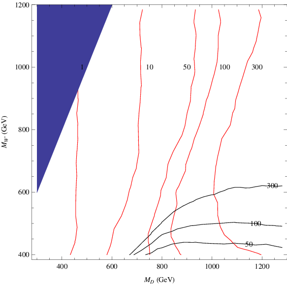
One can see that almost the entire parameter space is covered, with the pair and single production channels nicely complementing each other. Before we conclude, however, we would like to comment briefly on how our analysis compares with other models with vector quarks.

VIII Related Vector Quark Models

There are many other theories that feature heavy quarks with vector like couplings, as in the present model. In this section, we would like to briefly explain how our phenomenological analysis compares with these. One important feature of deconstructed Higgsless models of the kind discussed in this paper is ideal fermion delocalization, which does not allow the heavy charged gauge bosons in the theory to couple to two standard model fermions. This constrains the $W^{\prime}$ to decay only to $W$ and $Z$ , thus providing a tool to distinguish this class of models from others. There are, however, certain features of this model that are generic, like the vector nature of the heavy quark couplings.

In the context of Little Higgs Models [59], there have been studies of the LHC phenomenology of the T-odd heavy quarks [60]. The cross sections for the production of heavy T-quark pairs are comparable to the ones in our study. However, in those models, the heavy T-quark necessarily decays to a heavy photon (due to constraints of conserving T parity). Also, in [61], the authors study the pair production of heavy partners of the 1st and 2nd generation quarks in the context of the Littlest Higgs Models [62, 63, 64, 65]. They consider decays exclusively to the heavy gauge bosons in the theory, which then decay to the standard model gauge bosons plus a heavy photon. Thus, the final state, though still $llljjE\!\!\!\!/\ _{T}$ , is kinematically different. In particular, strong cuts on the missing energy are now an important part of the analysis, because part of $E\!\!\!\!/\ _{T}$ is due to the heavy photons. Ref.[66] presents a comprehensive study of the production and decay of heavy quarks by separating out the partners of the 3rd generation from the others and analysing them separately. The authors let the heavy quark decay to a SM $W$ boson and a light quark, but in their analysis, they neglect the mass of the $W$ boson compared to its momentum (since it is highly boosted). Thus, when the $W$ decays to a $l\nu$ pair, the direction of the neutrino momentum can be approximated to be parallel to that of the charged lepton, which enables them to recontruct the full neutrino momentum and create an invariant mass peak for the heavy quark (as opposed to a transverse mass analysis). Clearly, the final states and/or kinematics in all of these analyses differ significantly from those considered in our analysis.

In the context of the three site model, the authors of [67] consider the single production of the heavy top quark. As mentioned before, the heavy top in this model is necessarily around a few TeV’s and the paper concludes that the most viable channel for detection at the LHC is the subprocess $qb\rightarrow q^{\prime}T\rightarrow q^{\prime}Wb$ with the $W$ decaying leptonically. We have not yet studied heavy top or top-pion phenomenology in our model.

Ref. [68] presents a model independent analysis of the discovery prospects of heavy quarks at the Tevatron. The authors write down generic charged and neutral current interactions mixing the heavy and the light fermions and proceed to analyze both the pair and single production of these heavy quarks, with decays to the SM gauge bosons. Understandably, the Tevatron reach is much lower than that of the LHC.

IX Discussions & Conclusions

Higgsless models have emerged as an alternative to the Standard Model in explaining the mechanism of electroweak symmetry breaking. These theories use boundary conditions to break gauge symmetries and can be understood in terms of four dimensional gauge theories via the process of deconstruction. A minimal model along these lines was recently presented [24], which employed just three sites. A natural feature of this model was the presence of partners to the SM fermions whose masses were of the order of a few TeV or more, because of the twin constraints of getting the top quark mass right and having the $\rho$ parameter under experimental bounds.

In this paper, we presented a minimal extension of the three site model that incorporates both Higgsless and top-color mechanisms. The model singles out top quark mass generation as arising from a Yukawa coupling to an effective Top-Higgs, which develops a small vacuum expectation value, while electroweak symmetry breaking results largely from a Higgsless mechanism. An interesting consequence is that there is no longer a conflict between the need to obtain a realistically large value for the top quark mass and the need to keep $\Delta\rho$ small enough to conform to experiment. As a result, in this model it is possible to have additional vector-like quarks in the model that are light enough to be discovered at the LHC, without affecting the tree level couplings of the three site model too much.

We encoded the model in CalcHEP and analyzed the phenomenology of the heavy quarks. We first considered pair production ( $pp\rightarrow Q\bar{Q}\rightarrow WZjj\rightarrow lll\nu jj$ ) of these heavy fermions. We found that the 5 $\sigma$ reach of the pair production channel was $\approx$ 1 TeV, with the maximum reach in the region where $M_{W^{\prime}}>M_{Q}$ where the heavy quark must decay to a $W$ or $Z$ . The single production channel ( $pp\rightarrow Qj\rightarrow W^{\prime}jj\rightarrow WZjj\rightarrow lll\nu jj$ ) complements this nicely because we can study the decay of the heavy quark to a $W^{\prime}$ , and hence are necessarily in the region $M_{W^{\prime}}<M_{D}$ . By combining both these analyses, we were able to cover most of the $M_{D}-M_{W^{\prime}}$ parameter space. We conclude that the reach at the LHC for a 5 $\sigma$ discovery at 95% c.l. of the vector quarks in this theory can be as high as 1.2 TeV for an appropriate choice of $M_{W^{\prime}}$ .

Other components of the theory with potentially interesting phenomenology are the heavy partners of the $B$ and $T$ quarks and the uneaten top pions that arise from the extra link in the Moose diagram (Figure 1) and couple preferentially to the third generation. The phenomenology of these states is currently under investigation.

Acknowledgements.

This work was supported in part by the US National Science Foundation under grant PHY-0354226. BC acknowledges Chuan-Ren Chen for useful discussions during the initial stages of this project. NDC would like to thank James Linnemann and James Kraus for helpful discussions during the final stages of this project. RSC and EHS gratefully acknowledge the hospitality and support of the Aspen Center for Physics where some of this work was completed. All the Feynman diagrams in this paper were generated using JaxoDraw [69, 70].

References

[1] P. W. Higgs, Phys. Lett. 12 (1964) 132-133.
[2] C. Csaki, C. Grojean, H. Murayama, L. Pilo and J. Terning, Phys. Rev. D 69, 055006 (2004) [arXiv: hep-ph/0305237].
[3] K. Agashe, A. Delgado, M. J. May and R. Sundrum, JHEP 0308, 050 (2003) [arXiv:hep-ph/0308036].
[4] C. Csaki, C. Grojean, L. Pilo and J. Terning, Phys. Rev. Lett. 92 (2004) 101802 [arXiv: hep-ph/0308038].
[5] G. Burdman and Y. Nomura, Phys. Rev. D 69, 115013 (2004) [arXiv: hep-ph/0312247].
[6] G. Cacciapaglia, C. Csaki, C. Grojean and J. Terning, Phys. Rev. D 70, (2004) 075014 [arXiv: hep-ph/0401660].
[7] J. M. Maldacena, Adv. Theor. Math. Phys. 2 (1998) 231-252 [arXiv: hep-th/9711200].
[8] S. S. Guber, I. R. Klebanov and A. M. Polyakov, Phys. Lett. B 428 (1998) 105-114 [arXiv: hep-th/9802109].
[9] E. Witten, Adv. Theor. Math. Phys. 2 (1998) 253-291 [arXiv: hep-th/9802150].
[10] O. Aharony, S. S. Guber, J. M. Maldacena, H. Ooguri and Y. Oz, Phys. Rept. 323 (2000) 183-386 [arXiv: hep-th/9903394].
[11] N. Arkani-Hamed, A. G. Cohen and . Georgi, Phys. Rev. Lett. 86 (2001) 4757-4761 [arXiv:hep-th/0104005].
[12] C. T. Hill, S. Pokorski and J. Wang, Phys. Rev. D 64 (2001) 105005 [arXiv: hep-th/0104035].
[13] R.S. Chivukula, D. A. Dicus and H.-J. He, Phys. Lett. B525 (2002) 175-182 [arXiv: hep-ph/0111016].
[14] R.S. Chivukula and H.-J. He, Phys. Lett. B532 (2002) 121-128 [arXiv: hep-ph/0201164].
[15] R.S. Chivukula, D. A. Dicus H.-J. He and S. Nandi, Phys. Lett. B562 (2003) 109-117 [arXiv: hep-ph/0302263].
[16] H.-J.He, arXiv: hep-ph/0412113.
[17] R. S.Chivukula, E. H. Simmons, H.-J. He, M. Kurachi and M. Tanabashi, Phys. Rev. D 71 (2005) 035007 [arXiv: hep-ph/0410154].
[18] G. Cacciapaglia, C. Csaki, C. Grojean and J. Terning, Phys. Rev. D 71, (2005) 035015 [arXiv: hep-ph/0409126].
[19] G. Cacciapaglia, C. Csaki, C. Grojean, M. Reece and J. Terning, Phys. Rev. D 72, (2005) 095018 [arXiv: hep-ph/0505001].
[20] R. Foadi, S. Gopalakrishna and C. Schmidt, Phys. Lett. B 606 (2005) 157 [arXiv: hep-ph/0409266].
[21] R. Casalbuoni, S. De Curtis, D. Dolce and D. Dominici, Phys. Rev. D 71, 075015 (2005) [arXiv:hep-ph/0502209].
[22] R. Foadi, and C. Schmidt, An Effective Higgsless Theory: Phys. Rev. D 73 (2006) 075011 [arXiv: hep-ph/0509071].
[23] R. S. Chivukula, E. H. Simmons, H.-J. He, M. Kurachi and M. Tanabashi, Phys. Rev. D 72 (2005) 015008 [arXiv: hep-ph/0504114].
[24] R. S. Chivukula, B. Coleppa, S. Di Chiara, E. H. Simmons, H.-J. He, M. Kurachi and M. Tanabashi, Phys. Rev. D 74 (2006) 075011 [arXiv: hep-ph/0607124].
[25] C. T. Hill, Phys. Lett. B 266 , 419-424 (1991)
[26] C. T. Hill and S. Parke, Phys. Rev. D49, 4454 (1994).
[27] H. Georgi, Nucl. Phys. B266 (1986) 274.
[28] A.S. Belyaev, R.S. Chivukula, N.D. Christensen, H.-J. He, M. Kurachi, E.H. Simmons, and M. Tanabashi, $W_{L}W_{L}$ Scattering in Higgsless Models: Identifying Better Effective Theories, In preparation. June 2009.
[29] R. Casalbuoni, S. De Curtis, D. Dominici, and R. Gatto, stron higgs sector, Phys. Lett. B155 (1985) 95.
[30] R. Casalbuoni et. al., of a low energy strong electroweak sector, Phys. Rev. D53 (1996) 5201-5221 [hep-ph/9510431].
[31] M. Bando, T. Kugo, S. Uehara, K. Yamawaki, and T. Yanagida, Is rho meson a dynamical gauge boson of hidden local symmetry?, Phys. Rev. Lett. 54 (1985) 1215.
[32] M. Bando, T. Kugo, and K. Yamawaki, Nucl. Phys. B259 (1985) 493.
[33] M. Bando, T. Kugo, and K. Yamawaki, Phys. Rept. 164 (1988) 217-314.
[34] M. Bando, T. Fujiwara, and K. Yamawaki, Prog. Theor. Phys. 79 (1988) 1140.
[35] M. Harada and K. Yamawaki, Phys. Rept. 381 (2003) 1-233 [hep-ph/0302103].
[36] Y. Nambu, Proc. 1988 Int. Workshop on New Trends in Strong Coupling Gauge theories, Nagoya, Japan, Aug 24-27, 2988.
[37] V. A. Miransky, M. Tanabashi and K. Yamawaki, Phys. Lett. B 221, 177 (1989).
[38] V. A. Miransky, M. Tanabashi and K. Yamawaki, Mod. Phys. Lett. A 4, 1043 (1989).
[39] W. J. Marciano, Phys. Rev. D 41, 219 (1990).
[40] W. A. Bardeen, C. T. Hill and M. Lindner, Phys. Rev. D 41, 1647 (1990).
[41] W. J. Marciano, Phys. Rev. Lett. 62, 2793 (1989).
[42] C. T. Hill and E. H. Simmons, Phys. Rept. 381: 235-402 (2003), Erratum-ibid. 390: 553-554 (2004) [arXiv: hep-ph:0203079].
[43] C. T. Hill, B 345: 483-489 (1995) [hep-ph/9411426].
[44] K. Lane and E. Eichten, Phys. Lett. B 352: 382-387 (1995).
[45] M. B. Popovic and E. H. Simmons, Phys. Rev. D 58, 095007 (1998) [arXiv:hep-ph/9806287].
[46] F. Braam, M. Flossdorf, R. S. Chivukula, S. Di Chiara and E. H. Simmons, Phys. Rev. 77, 055005 (2008) [arXiv:0711.1127 [hep-ph]].
[47] B. A. Dobrescu and C. T. Hill, Phys. Rev. Lett. 81, 2634 (1998) [arXiv:hep-ph/9712319].
[48] R. S. Chivukula, B. A. Dobrescu, H. Georgi, and C. T. Hill, Phys. Rev. D 59: 075003 (1999) [hep-ph/9809470].
[49] A. Aranda and C. D. Carone, Int. J. Mod. Phys. A16S1C, 899-901 (2001) [hep-ph/0010279].
[50] A. Aranda and C. D. Carone, Phys. Lett. B488: 351-358 (2000).
[51] Hong-Jian He, Yu-Ping Kuang, Yong-Hui Qi, Bin Zhang, Alexander Belyaev, R.Sekhar Chivukula, Neil D. Christensen, Alexander Pukhov and Elizabeth H. Simmons, Phys. Rev. D78, 031701 (2007) [arXiv: 0708.2588 [hep-ph]].
[52] T. Ohl and C. Speckner, Phys. Rev. D 78, 095008 (2008) [arXiv:0809.0023 [hep-ph]].
[53] E. Eichten and K. D. Lane, Phys. Lett. B 90, 125 (1980).
[54] S. Dimopoulos and L. Susskind, Nucl. Phys. B 155, 237 (1979).
[55] K. Agashe, M. Papucci, G. Perez and D. Pirjol, arXiv:hep-ph/0509117.
[56] “Search for Heavy Top t’ $\rightarrow$ Wq in Lepton Plus Jets Events”, CDF-note-9234; T. Aaltonen et al. [CDF Collaboration], Phys. Rev. D 76, 072006 (2007).
[57] A. Pukhov, arXiv: hep-ph/0412191.
[58] J. Bagger, et al., Phys. Rev. D 52, 3878 (1995).
[59] N. Arkani-Hamed, A. G. Cohen, and H. Georgi, Phys. Lett. B 513, 232 (2001); For reviews, see, for example, M. Schmaltz and D. Tucker Smith, Ann. Rev. Nucl. Part. Sci. 55, 229 (2005); M. Perelstein, Prog. Part. Nucl. Phys. 58, 247 (2007) and references within.
[60] M. S. Carena, J. Hubisz, M. Perelstein, and P. Verdier, Phys. Rev. D79: 091701 (2007) [hep-ph/0610156].
[61] D. Choudhury, and D. K. Ghosh, JHEP 0708: 084 (2007) [hep-ph/0612299].
[62] I. Low, JHEP 0410, 067 (2004).
[63] J. Hubisz, and P. Meade, Phys. Rev. D 71: 035016 (2005) [hep-ph/0411264].
[64] J. Hubisz, P. Meade, A. Noble, and M. Perelstein, JHEP 0601: 135 (2006) [hep-ph/0506042].
[65] H. C. Cheng, and I. Low, JHEP 0309: 051 (2003); JHEP 0408: 061 (2004).
[66] Tao Han, Heather E. Logan, and Lian-Tao Wang, JHEP 0601: 099 (2006), [hep-ph/0506313].
[67] Chong-Xing Yue, Li-Hong Wang, and Jia Wen, Chin. Phys. Lett, 25: 1613-1616 (2008) [arXiv: 0708.1225].
[68] Anupama Atre, Marcela Carena, Tao Han, and Jose Santiago, Heavy Quarks Above the Top at the Tevatron, arXiv:0806.3966 [hep-ph].
[69] D. Binosi and L. Theussl, JaxoDraw: A graphical user interface for drawing Feynman diagrams, Comput. Phys. Commun. 161: 76-86 (2004) [hep-ph/0309015].
[70] D. Binosi, J. Collins, C. Kaufhold, and L. Theussl, JaxoDraw: A graphical user interface for drawing Feynman diagrams, Version 2.0 release notes [arXiv: 0811.4113].