The Hierarchy of Incompressible Fractional Quantum Hall States

Solid state theory has developed from the realization [117] that simple metals could be described in terms of free electrons that obeyed the Pauli exclusion principle [86]. Very early work on the effect of the periodic potential of the solid on the single electron eigenstates [8] led to the concept of energy bands and bandgaps [126], and to understanding of why some solids were metals while others were insulators, semiconductors or semimetals [131]. The early decades of solid state physics were dominated by this “single particle” description of electronic states.

In the middle of the last century scientists began to worry about why this single particle picture worked so well, since the interaction between particles was not so small. Landau [53, 54] proposed the Fermi liquid theory to describe the effect of short range many body interaction in liquid $\rm{He}^{3}$. The concept of quasiparticles (QPs), elementary excitations that satisfied Fermi-Dirac statistics and included a “self-energy” (due to interaction with the ground-state) and a weak interaction with one another, became a critical new concept in solid state theory. Silin [110] made use of Landau’s idea to study the properties of a ”metallic” electron liquid with long range Coulomb interactions. In microscopic studies of the electron liquid many-electrons interactions were treated via diagrammatic perturbation theory. The starting point, however, was still the single electron eigenstates and the Fermi distribution function.

The BCS theory of superconductivity [5] demonstrates that perturbation theory was not always adequate, even when interactions were weak. However, even in BCS theory the noninteracting electron states served as the starting point for introduction of novel correlation effects via a generalized mean field approximation.

During the past two decades novel systems have been discovered in which many-body interaction appears to dominate over single particle energies. Transition metal oxides displaying a metal-insulator transition, magnetic phase transitions and high temperature superconductivity are one technologically important class of such “strongly interacting systems”. When interactions dominate, the standard technique of treating them as a perturbation on the single particle spectrum is usually not adequate.

The paradigm for such systems is the fractional quantum Hall (FQH) system. At very high values of the applied magnetic field the massively degenerate single particle Landau levels (LLs) disappear from the problem. The low energy spectrum is determined by a single energy scale $e^{2}/\lambda$, where $\lambda=(\hbar c/eB)^{1/2}$ is the magnetic length. The incompressible quantum liquid (IQL) states discovered by Tsui et al. [124] result from the interaction alone.

In this paper we present a review of the families of FQH states observed experimentally and of how we understand them. Although a lot of theoretical methods have been developed, we would limit ourselves to those that are critical to our explanations, leaving out for example some work rooted in field theories [4, 28, 64, 65, 66, 67] and Hamiltonian method [80, 109, 78, 79]. Laughlin’s remarkable insight [56] into the nature of correlations giving rise to an IQL state and the fractionally charged excitations: quasielectrons (QEs) and quasiholes (QHs) are discussed. We consider Haldane’s idea [37] that a hierarchy of IQL daughter states can be attributed to the fact that putting fractionally charge QPs into a QP Landau level is essentially the same problem as that of putting the original electrons in an electron Landau level. We review Jain’s remarkable composite Fermion (CF) picture [46]. It predicts not only the filling factor $\nu$ at which the most prominent IQL states are observed, but structure of the lowest band of energy states for any value of the applied magnetic field $B$. We emphasize the conditions under which the CF picture is valid and discuss why it’s valid. We give examples in which the CF picture is not valid. We suggest that a useful approach to many Fermion systems dominated by the interaction between pairs is to study the antisymmetric eigenstates of a single pair and to use them to construct an appropriate product over all pairs. For the simplest case, this is exactly the Laughlin wavefunction, a better starting point for a many Fermion system than a Slater determinant of single particle wavefunctions. We propose novel correlations, different from Laughlin’s, when the pair interactions are different from the Coulomb interaction in the lowest Landau level (LL0).

Our objective is to give a deeper intuitive understanding of all FQH states in the hope that it may suggest novel ways to treat correlations in other strongly interacting systems.

The integral quantum Hall (IQH) effect was discovered by von Klitzing et al. [51] who investigated the magnetotransport properties of a quasi two dimensional (2D) electron gas in a silicon surface inversion layer.

The Hamiltonian describing the motion of a single electron confined to the $x-y$ plane in the presence of a dc magnetic field $\vec{B}=B\hat{z}$ is simply $H=(2\mu)^{-1}[\vec{p}+(e/c)\vec{A}(\vec{r})]^{2}$. The vector potential $\vec{A}(\vec{r})$ in the symmetric gauge is given by $\vec{A}(\vec{r})=(1/2)B(-y\hat{x}+x\hat{y})$. We use $\hat{x},~\hat{y}~,$ and $\hat{z}$ as unit vectors along the Cartesian axes. The Schrödinger equation $(H-E)\Psi(\vec{r})=0$ [55] has eigenstates:

The radial wavefunction $u_{nm}(r)$ can be written as

where $x^{2}=1/2(r/\lambda)^{2}$, and $L_{n}^{|m|}$ is an associated Laguerre polynomial. $L_{0}^{|m|}$ is independent of $x$, and $L_{1}^{|m|}$ is proportional to $(|m|+1-x^{2})$. From Eq. 2 it is apparent that the spectrum of single-particle energies consists of highly degenerate levels; the lowest LL has $n=0$ and $m=0,-1,-2,\ldots$, and its wavefunction can be written $\Psi_{0m}=z^{|m|}\exp[-|z|^{2}/4/\lambda^{2}]$, where $z$ stands for $re^{-i\phi}$. For a finite-size sample of area $\mathcal{A}$, the number of single-particle states in the lowest LL is given by $N_{\phi}=B\mathcal{A}/\phi_{0}$, where $\phi_{0}=hc/e$ is the quantum of flux. The filling factor $\nu$ is defined as $N/N_{\phi}$, so that $\nu^{-1}$ is simply equal to the number of flux quanta of the magnetic field per electron.

When $\nu$ is equal to an integer, there is an energy gap (equal to $\hbar\omega_{c}$) between the filled states and the empty states. This makes the noninteracting electron system incompressible, because an infinitesimal decrease in the area $\mathcal{A}$ can be accomplished only at the expense of promoting an electron across the energy gap and into the first unoccupied LL. This incompressibility is responsible for the integral quantum Hall effect [50].

In Fig. 1 we display typical results for $V_{X}$, the voltage along the channel, and $V_{H}$, the Hall voltage. The former contains zeros at the integral values of the filling factor $\nu$ caused by the energy gap between the filled and empty LLs. Both localized and extended states occur in the LLs. When the chemical potential $\zeta$ resides in the localized states $\sigma_{xx}$ vanishes (at T=0), and since localized states make no contribution, the Hall conductivity $\sigma_{xy}$ remains constant as $\zeta$ moves through the localized states. The integral value of $\sigma_{xy}$ in units of $e^{2}/h$ is expected when $\nu$ is precisely equal to an integer. The Hall plateaus depend on the spectrum of the localized states which is related to the mobility of the sample.

The observation of an incompressible quantum Hall liquid state in a fractionally filled 2D Landau level by Tsui et al. [124] was quite unexpected. The behavior of $\rho_{xx}$ and $\rho_{xy}$ as a function of filling factor $\nu$ is displayed for a typical early measurement in Fig. 2. There are clear zeroes of $\rho_{xx}$ at $\nu=1/3$ and $2/3$ and corresponding plateaus in $\rho_{xy}$. At other fractions there are observable minima in $\rho_{xx}$ and changes in slope in $\rho_{xy}$. The trace looks like a continuation of Fig. 1 to higher magnetic field or lower filling factor. Later, with significant improvement of the quality of the sample, other filling fractions have been observed in both lowest Landau level [81], and higher LL [130, 82, 161, 18]. Unlike the IQH effect, the FQH effect cannot be understood in terms of the single particle spectrum. Coulomb correlations among electrons in the partially filled LL of degenerate single particle states must be responsible for the incompressibility (and the energy gap associated with it). Clearly, this is a novel many-body state.

Laughlin [56] correctly surmised that the FQH states observed at filling factors $\nu=m^{-1}$, with $m$ being an odd integer, resulted when the electrons were able to avoid pair states with relative angular momentum smaller than $m$. These avoided pair states have the smallest pair separation and the largest Coulomb repulsion. Laughlin proposed a many-body wavefunction for the IQL state at filling factor $\nu=m^{-1}$ given by

Here $z_{i}=r_{i}e^{-i\phi_{i}}$ is a complex coordinate for the position of the $i^{\rm{th}}$ electron, $\lambda$ is the magnetic length and $z_{ij}=z_{i}-z_{j}$. Clearly, in going from the filled $\nu=1$ state to the $\nu=1/3$ state, the Laughlin wavefunction has introduced two additional zeroes as a function of pair separation $|z_{ij}|$. The relative pair angular momentum is simply $m$, the $z$-component of the relative angular momentum of particles $i$ and $j$. Laughlin also showed that the elementary excitations of the IQL state could be described as fractionally charged QEs and QHs. Both localized and extended states of the quasiparticles were required to understand the observed behavior of $\rho_{xx}$ and $\rho_{xy}$.

The first explanation of FQH states at values of $\nu=n(1+2p)^{-1}$ with $n>1$ was given by Haldane [37]. He assumed that the dominant interaction between quasiparticles was the short range repulsive part of the pair interaction. Based on this assumption Haldane suggested that the problem of filling the degenerate states of the QP LL with $N_{\rm{QP}}$ Laughlin quasiparticles was similar to that of filling the original $N_{\phi}$ states of the electron LL with $N$ electrons. Because the number of QP states could not exceed $N$, Haldane suggested the $N$ took place of $N_{\phi}$ and $N_{\rm{QP}}$ the place of $N$ in the Laughlin’s condition $N_{\phi}=(2p+1)N$ for an IQL state. He proposed $N=2pN_{\rm{QP}}$ as the condition for new IQL states of the QPs. The even integer $2p$ was chosen because, according to Haldane, the QPs were Bosons. This “Haldane hierarchy” of IQL states contained all odd denominator fractions. Slightly different versions of Haldane’s hierarchy were independently suggested by Laughlin [57] and by Halperin [41, 40]. The different versions differ in the definition of the relative angular momentum of QPs, resulting in different assignment of QP statistics. All of the versions depended on the residual interactions between QPs (which were not well-known) being sufficiently similar to the Coulomb interactions between electrons in LL0.

Confirmation of Laughlin’s explanation of the correlations giving rise to FQH states at $\nu=1/3,1/5,\ldots$ can be found through numerical diagonalization of the Coulomb interaction within the subspace of the lowest LL. Higher LLs play almost no role in the low energy spectrum if the cyclotron energy $\hbar\omega_{c}$ is much larger than the Coulomb energy $e^{2}/\lambda$. Exact numerical diagonalization is limited to small systems, but it must give qualitatively correct results as long as the correlation length is much smaller than the radius of the system. Restricting the area of the sample can be done in different ways, but probably the most useful is to make the 2D surface on which the electrons reside a sphere of radius $R$ [37, 39]. In this geometry a magnetic monopole of strength $2Q\phi_{0}$ (where $2Q$ is an integer) at the center of sphere gives a radial magnetic field $B=2Q\phi_{0}/4\pi R^{2}$. Boundary conditions are avoided and the rotational invariance replaces the translational invariance of an infinite plane.

The single particle eigenstates (called monopole harmonics [158, 159]) are denoted by $|Q,\ell,m>$, where the angular momentum $l$ and its $z$-component $m$ must satisfy $|m|\leq l$. The single particle eigenvalues are given by $E_{l}=(\hbar\omega_{c}/2Q)[\ell(\ell+1)-Q^{2}]$. Since $E_{l}$ cannot be negative, the minimum allowed value of $\ell$ must be $Q$. We can write $\ell=Q+n$, with $n=0,1,\ldots$ playing the role of LL index. For $\nu<1$ only the lowest LL (with $\ell=Q$) is relevant at high magnetic fields. We can write $N$ electron basis states as: $|m_{1},m_{2},\ldots,m_{N}>=c_{m_{N}}^{{\dagger}}\ldots c_{m_{2}}^{{\dagger}}c_{m_{1}}^{{\dagger}}|vac>$, where $|vac>$ is the vacuum state and $c_{m}^{{\dagger}}$ creates an electron in state $|Q,\ell,m>$ with $\ell=Q$. Of course the allowed values of $m$ must satisfy $|m|\leq\ell$. Although the two body matrix elements of the Coulomb interaction $<m_{1},m_{2}|V|m_{3},m_{4}>$ have a simple form in the lowest Landau level [26], the number of $N$ electron states $[N_{\phi}!/N!(N_{\phi}-N)!]$ grows rapidly with the system size. In the lowest LL where $\ell=Q$ the $N$-electron states can be written $|L,L_{z},\alpha>$ with $L$ and $L_{z}$ being the total angular momentum and its $z$ component, and $\alpha$ is an index that distinguishes different multiplets with the same value of $L$. Because the Coulomb interaction Hamiltonian $H=\sum_{i<j}V(|\vec{r}_{i}-\vec{r}_{j}|)$ is spherically symmetric, the Wigner-Eckart theorem tells us that $<L^{\prime},L^{\prime}_{z},\alpha^{\prime}|H|L,L_{z},\alpha>=\delta(L^{\prime},L)\delta(L^{\prime}_{z},L_{z})V_{\alpha\alpha^{\prime}}(L)$, and the reduced matrix element $V_{\alpha\alpha^{\prime}}$ is independent of $L_{z}$. This fact can be used to reduce the size of matrices to be diagonalized [137, 98].

It is probably worth noting that on a plane [137] the allowed values of $m$, the $z$-component of the single particle angular momentum, are $0,1,\ldots,N_{\phi}-1$. $M=\sum_{i}m_{i}$ is the total $z$-component of the angular momentum (the sum is over occupied states). It can be divided into $M_{\rm{CM}}+M_{\rm{R}}$, the center of mass and relative contributions. The connection between the planar and spherical geometries is $M=N\ell+L_{z}$, $M_{R}=N\ell-L$, and $M_{\rm{CM}}=L+L_{z}$. The interactions depend only on $M_{\rm{R}}$ so $|M_{\rm{R}},M_{\rm{CM}}>$ acts just like $|L,L_{z}>$. The absence of boundary conditions and the complete rotational symmetry make the spherical geometry attractive to theorists. Many experimentalists prefer using the $|M_{\rm{R}},M_{\rm{CM}}>$ states of the planar geometry.

Some exact diagonalization results ($E$ vs. $L$) for the ten electron system are shown in Fig. 3. The Laughlin $L=0$ incompressible ground state occurs at $2Q=3(N-1)$ for the $\nu=1/3$ state. States with larger values of $Q$ contain one or two QHs ($2Q=28,29$), and states with smaller values of $Q$ contain QEs in the ground states [91, 98, 92].

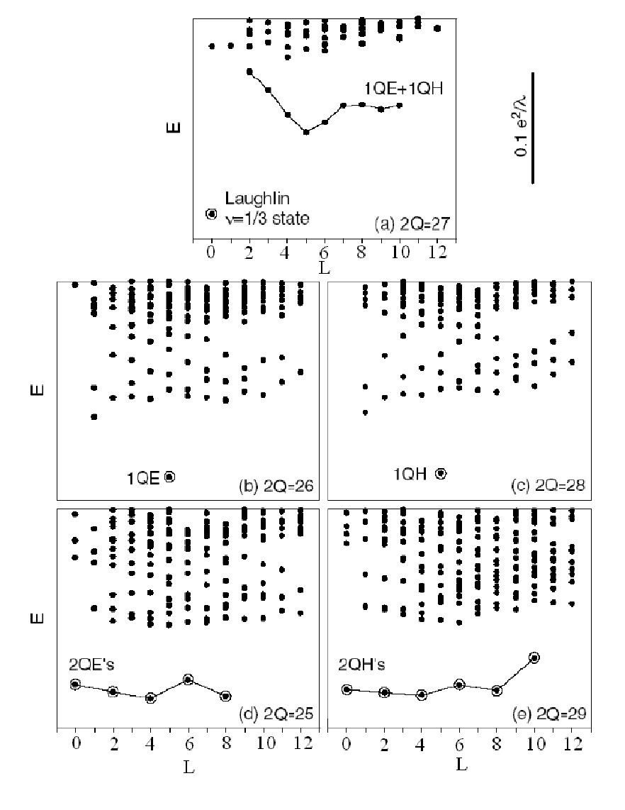
The energy of the multiplet $|L\alpha>$ can be expressed as

where $P_{L\alpha}(L^{\prime})$ is the probability that $|L\alpha>$ contains pairs with pair angular momentum $L^{\prime}$, and $V(L^{\prime})$ is the energy of interaction of a pair with angular momentum $L^{\prime}=2\ell-\mathcal{R}$. Here $R=1,3,5,\ldots$ is referred to as the relative pair angular momentum. We will sometimes use the notation $V(\mathcal{R})$ understanding this to mean $V(2\ell-\mathcal{R})$ i.e. the function $V(L^{\prime})$ with $L^{\prime}$ expressed as $2\ell-\mathcal{R}$.

It is straightforward to evaluate the pseudopotential $V(\mathcal{R})$ describing the interaction of a pair of electrons in a shell of angular momentum $l$ in the Haldane spherical geometry [26]. It depends on the radius of the sphere $R=(Q)^{1/2}\lambda$ and on the Landau level index $n=\ell-Q=0,1,2,\ldots$. Simple results for $V^{(n)}(\mathcal{R})$ are given in Fig. 4.

Jain [46] made the remarkable observation that the most prominent IQL states observed experimentally could be understood in terms of a simple composite Fermion (CF) picture. This picture made use of a Chern–Simons (CS) transformation [127, 128] and a CS gauge field familiar to field theorists. The CS transformation can be described as attaching to the $j^{\rm{th}}$ electron $(1\leq j\leq N)$ a flux tube carrying a magnetic field $\vec{b}=\alpha\phi_{0}\delta(\vec{r}-\vec{r}_{j})\hat{z}$. Here $\phi_{0}=(hc)/e$ is the quantum of flux, $\alpha$ is a constant, and $\hat{z}$ a unit vector normal to the 2D layer. It is well-known that when this CS flux is added via a gauge transformation, no change in the classical equations of motion results. Only the phase of the quantum mechanical wavefunction is changed. However, the CS transformation results in a much more complicated many-body Hamiltonian that includes a CS vector potential $\vec{a}(\vec{r})$ given by

in addition to the vector potential $\vec{A}(\vec{r})$ of the dc magnetic field. Simplification results only when the mean field (MF) approximation is made. This is accomplished by replacing the density operator $\psi^{\dagger}(\vec{r})\psi(\vec{r})$ in the CS vector potential and in the Coulomb interaction by its MF value $n_{s}$, the uniform electron density. The resulting Hamiltonian is the sum of single particle Hamiltonians in which an “effective” magnetic field $B^{\ast}=B-\nu\phi_{0}n_{s}$ appears.

Jain introduced the idea of a CF to represent an electron with an attached flux tube which carried an even number $\alpha(=2p)$ of flux quanta [47]. In the MF approximation the CF filling factor $\nu^{\ast}$ is given by $\nu^{\ast-1}=\nu^{-1}-\alpha$, i.e. the number of flux quanta per electron of the dc field less the CS flux per electron. When $\nu^{\ast}$ is equal to an integer $n=\pm 1,\pm 2,\ldots$ , then $\nu=n(1+\alpha n)^{-1}$ generates (for $\alpha$=2) quantum Hall states at $\nu=1/3,2/5,3/7,\ldots$, and $\nu=1,2/3,3/5,\ldots$. These are the most pronounced FQH states observed.

In the spherical geometry one can introduce an effective monopole strength seen by one CF [16]. It is given by $2Q^{\ast}=2Q-\alpha(N-1)$ since the $\alpha$ flux quanta attached to every other CF must be subtracted from the original monopole strength 2$Q$. Then $|Q^{\ast}|=\ell_{0}^{\ast}$ plays the role of the angular momentum of the lowest CF shell just as $Q=\ell_{0}$ is the angular momentum of the lowest electron shell. When $2Q$ is equal to an odd integer $(1+\alpha)$ times $(N-1)$, the CF shell $\ell_{0}^{\ast}$ is completely filled, and an $L=0$ incompressible Laughlin state at filling factor $\nu=(1+\alpha)^{-1}$ results. When $2|Q^{\ast}|+1$ is smaller (larger) than $N$, QEs (QHs) appear in the shell $\ell_{\rm{QE}}=\ell^{\ast}_{0}+1~(\ell_{\rm{QH}}=\ell_{0}^{\ast})$. The low energy sector of the energy spectrum consists of the states with the minimum number of QP excitations required by the value of 2$Q^{\ast}$ and $N$. The first excited band of states will contain one additional QE-QH pair. The total angular momentum of these states in the lowest energy sector can be predicted by addition of the angular momenta ($\ell_{\rm{QH}}$ or $\ell_{\rm{QE}}$) of the $n_{\rm{QH}}$ or $n_{\rm{QE}}$ quasiparticles treated as identical Fermions. In Table 1 we demonstrated how these allowed $L$ values are found for a ten electron system with $2Q$ in the range $29\geq 2Q\geq 25$. By comparing with numerical results presented in Fig. 3, we readily observe that the total angular momentum multiplets appearing in the lowest energy sector are always correctly predicted by this simple MF CS picture [91, 98, 92].

For example, the Laughlin $L=0$ ground state at $\nu=1/3$ occurs when $2\ell_{0}^{\ast}=N-1$, so that the $N$ composite Fermions fill the lowest shell (with angular momentum $\ell_{0}^{\ast}$). The CFQE and CFQH states occur at $2\ell_{0}^{\ast}=N-1\mp 1$ and have one too many (for QE) or one too few (for QH) particles to give integral filling. The single QPs have angular momentum $N/2$. The 2QE and 2QH states occur at $2\ell_{0}^{\ast}=N-1\mp 2$. They have $\ell_{\rm{QE}}=(N-1)/2$ and $\ell_{\rm{QH}}=(N+1)/2$. We expect, for example, $\ell_{\rm{QE}}=4.5$ and $\ell_{\rm{QH}}=5.5$ for a ten electron system, leading to low energy bands with $L=0\oplus 2\oplus 4\oplus 6\oplus 8$ for 2 QEs and to $L=0\oplus 2\oplus 4\oplus 6\oplus 8\oplus 10$ for 2 QHs. In the MF picture, which neglects QP-QP interactions, these bands are degenerate. Of course, numerical results in Fig. 3 show that two QP states with different $L$ have different energy. From this numerical data we obtain, up to an overall constant, $V_{\rm{QP}}$ the residual interaction of a QP pair as a function of the pair angular momentum $L^{\prime}$ [91, 98, 92, 143].

In addition to the lowest energy band of multiplets, first excited bands which contain one additional QE-QH pair can be observed in Fig. 3. The “magnetoroton” band lying between the $L$=0 Laughlin IQL ground state and a continuum of higher energy states can be observed in Fig. 3(a). This band contains one QH with $\ell_{\rm{QH}}=9/2$ and one QE with $\ell_{\rm{QE}}=11/2$. By adding the angular momenta of these distinguishable particles, a band with $1=\ell_{\rm{QE}}-\ell_{\rm{QH}}\leq L\leq\ell_{\rm{QE}}+\ell_{\rm{QH}}=10$ would be predicted. The state with $L=1$ does not appear in Fig.3 (a) suggesting that QE-QH pairs with $L=1$ are forbidden (or at least pushed into the higher energy continuum by interactions). Furthermore, the states in the band are not degenerate indicating residual interactions that depend on the angular momentum of the pair. Other bands that are not quite so clearly defined can be observed in other frames. For example, in frame (b) between the single QE state at $L=5$ and the higher energy continuum, there is a 2QE-1QH band. The allowed $L$ values can be estimated by taking $\ell_{\rm{QE}}=5$ and $\ell_{\rm{QH}}=4$ and adding angular momenta (treating the QEs as identical Fermions). Interactions cause the predicted multiplets to overlap the bottom of the continuum for $3\leq L\leq 6$ but outside this range they are separate from it [91, 98, 92].

Despite the satisfactory description of the allowed angular momentum multiplets, the magnitude of the MFCF energies is completely wrong. The magnetoroton energy does not occur at the effective cyclotron frequency $\hbar\omega_{C}^{\ast}=eB^{\star}/mc$. . This MF energy is irrelevant at large values of $B$ (if we keep $m_{\rm{CF}}=m_{e}$), so it is a puzzle why the CF picture does so well at predicting the structure of the energy spectrum. It is interesting to compare the energy spectrum of $N$ noninteracting electrons with that of $N$ noninteracting CFs as done in Fig. 5.

For large values of $B$ the MF energy $\hbar\omega_{C}^{\ast}$ is much larger than the Coulomb scale $e^{2}/\lambda$. Therefore the low lying multiplets of interacting electrons will be contained in a band of width $e^{2}$/$\lambda$ about the lowest electron LL. The noninteracting CF spectrum contains a number of bands separated by $\hbar\omega_{C}^{\ast}$. Interactions (Coulomb and CS gauge interactions) among fluctuations beyond the MF essentially have to restore the original noninteracting electron spectrum when $B\rightarrow\infty$. Halperin et al.[42] and Lopez and Fradkin [64, 65, 66] have used conventional manybody perturbation theory to treat fluctuations. However, there is no small parameter to guarantee convergence or to justify simple approximations like the random phase approximation (RPA). The standard many-body perturbation theory gives reasonable results probably because it can be thought of as a Silin-Landau theory [53, 110] of an electron liquid. Long range correlations are handled by RPA; short range correlations by adding Landau Fermi liquid interactions [112]. What is clear is that the success of the CF picture does not result from a cancelation between CS gauge interactions and Coulomb interactions beyond MF.

Jain proposed a trial wavefunction which included a Jastrow factor $\prod_{i<j}z_{ij}^{2}$, and he projected it onto the lowest Landau level. He then diagonalized the Coulomb interaction using the projected trial function [47]. Though the technique seems to give reasonably good results, it is not obvious why it works.

The CS magnetic field $\vec{b}(\vec{r})=\alpha\phi_{0}\sum_{j}\delta(\vec{r}-\vec{r}_{j})\hat{z}$ is usually introduced via a gauge transformation. Then, it is a Bohm-Aharonov [1] type field, having no effect on the classical equation of motion. The Lorentz force on the $i^{\rm{th}}$ electron is given by $(-e/c)\vec{v}_{i}\times\vec{b}(\vec{r})$ with $\vec{r}=\vec{r}_{i}$. No electron senses its own CS flux, and since $\vec{r}_{i}$ and $\vec{r}_{j}$ cannot have the same value for a pair of Fermions, there is no effect from $\vec{b}(\vec{r})$ on the classical motion of the electrons. However, the CS flux does introduce a phase factor into the quantum mechanical wavefunction.

Let’s define $\psi_{m}(\vec{r})=\exp(im\phi)u_{m}(r)$ as the wavefunction for the relative coordinate $\vec{r}=\vec{r}_{i}-\vec{r}_{j}$ of pair electrons in the lowest LL. For Fermions $m$, the $z$-component of the relative angular momentum, must be odd so that under exchange $(\phi\rightarrow\phi+\pi)$ the phase factor changes sign. If a CS flux $\phi=\alpha\phi_{0}$ is introduced on each electron via a gauge transformation, then $\phi_{m}\rightarrow\exp[i(m-\alpha)\phi]u_{m}(r)$. The phase factor is changed by $\exp(-i\alpha\pi)\phi_{m}$ under exchange. If $\alpha$ is not an even integer this leads to the famous transmutation of statistics, since $\phi_{m}\rightarrow\exp(-i\alpha\pi)\phi_{m}$ under exchange [62, 129].

A gauge transformation is not the only way by which CS flux can be introduced. We can start with some initial state of the relative coordinates of pair, e.g. one with $\alpha=0$, and adiabatically increase the CS flux attached to each particle up to its final value. In this case $\phi_{m}$ evolves adiabatically into $\exp(im\phi)u_{m+\alpha}(r)$. There is no change in phase (and therefore no change in statistics for any value of $\alpha$). However, in the semiclassical orbit (described by maximum in the density $\rho(r)=|\phi_{m}|^{2}$) $u_{m}(r)$ is replaced by $u_{m+\alpha}(r)$. The orbit size changes in such a way that the total flux (due to both the applied field $B$ and the CS flux) is conserved. The change in orbit size results from the Faraday emf acting on the relative motion in the presence of perpendicular magnetic field $B$. If the pair was initially in the smallest allowed pair orbit (with $m=-1$) and two CS flux quanta opposite to $\vec{B}$ were added ($\alpha=-2$), then the resulting new orbit will have $m=-3$. This is exactly what we mean by Laughlin correlations. The adiabatic addition of CS flux has altered the orbit to avoid the most repulsive pair state with $m=-1$. However, in the absence of Coulomb interactions all negative values of $m$ belong to the lowest LL. No change in energy occurs without Coulomb repulsion. No MF approximation or MF energy scale is needed [90].

If we write the pair wavefunction as a product of center of mass (CM) and relative motion we find $\psi(\vec{r}_{i},\vec{r}_{j})=\exp(im\phi_{ij})u_{m}(r_{ij})u_{0}(R_{ij})$ can be written as $z_{ij}^{|m|}\exp[-(r_{i}^{2}+r_{j}^{2})/(4\lambda^{2})]$. Here $z_{i}=r_{i}\exp(-i\phi_{i})$ is the complex coordinate of the $i^{th}$ particle, and $\lambda^{2}=\hbar c/eB=2\lambda_{CM}^{2}=\lambda_{r}^{2}/2$. For an $N$ electron system the straightforward generalization of this pair function is the Laughlin wavefunction $\Phi_{m}(1,2,\ldots,N)=\prod_{i<j}z_{ij}^{|m|}\exp[-\sum_{k}r_{k}^{2}/(4\lambda^{2})]$ where $|m|$ is an odd integer. Small values of $|m|$ correspond to small pair orbits, with $|m|=1$ having the largest Coulomb repulsion. Adiabatic addition of CS flux to every electron forces each pair to be Laughlin correlated by avoiding pair orbits with $|m|=1$. This is accomplished without the necessity of a MF approximation or the introduction of a MF energy scale.

From our previous discussion we know that we can form total angular momentum multiplets $|\ell^{N};L\alpha>$ by addition of the angular momenta $\hat{\ell}_{i}=\hat{\ell}$ ($i=1,2,\ldots,N$) of $N$ Fermions. In the absence of Coulomb repulsion, $E_{\alpha}(L)$ is the same for every value of $L$ formed from $N$ electrons, each with angular momentum $\ell$ in the lowest LL (with $\ell=Q$, the monopole strength in the Haldane spherical geometry). Let’s define $G_{N\ell}(L)$ as the number of multiplets of total angular momentum $L$. If we adiabatically add two CS flux quanta to each electron, the $N$ particle multiplets that can be formed belong to a subset $G_{N\ell}(L)$ with $\ell$ replaced by $\ell^{\ast}=\ell-(N-1)$. The multiplets belonging to $G_{N\ell^{\ast}}(L)$ all avoid, to the maximum extend possibly, pair states with $\mathcal{R}=1$. This result is obviously true for a pair of Laughlin correlated electrons. The smallest allowed pair angular momentum would be $L^{\prime}=2\ell^{\ast}-1=2\ell-3$, completely avoiding $\mathcal{R}=1$. In addition our numerical results, (Fig. 3) show that the allowed values of $\ell_{\rm{QE}}$ and $\ell_{\rm{QH}}$ [frames (b) and (c)] are $\ell_{\rm{QE}}=\ell^{\ast}+1=5$ and $\ell_{\rm{QH}}=\ell^{\ast}=5$. This was easily understood in terms of “effective monopole strength”, but the result does not depend on the MF approximation. From frame (e) it is clear that $L_{2\rm{QH}}=2\ell^{\ast}-j$ where $j$ is an odd integer [and from (d) that $L_{2\rm{QE}}=2(\ell^{*}+1)-j$]. Thus, the adiabatic addition of CS flux introduces Laughlin correlations (avoiding $\mathcal{R}=1$) and selects [6, 94] from $G_{N\ell}(L)$ the subset $G_{N\ell^{*}}(L)$ that avoids the smallest (and most repulsive) pair orbit with $\mathcal{R}=1$. The proof that $G_{N\ell^{*}}(L)$ is a subset of $G_{N\ell}(L)$ has been given in Benjamin et al. [6].

When $N>2\ell^{\ast}+1$, there are more particles than can be accommodated in the lowest CF LL. An integral number of filled CF levels occurs when $N=n(2\ell^{*}+n)$, where $n=1,2,\ldots$. Then, the only state belonging to $G_{N\ell^{*}}(L)$ is the $L=0$ incompressible Jain state with filling factor $\nu=n(2n\pm 1)^{-1}$. This completely explains the Jain sequences $1/3,2/5,3/7,\ldots$ and $1,2/3,3/5,\ldots$ (though for simplicity we have considered $p=1$ instead of addition of $2p$ CS flux quanta). The gap between the lowest band of states (containing the minimum number of QPs required by the values of $2Q$ and $N$) and the first excited band is proportional to $V(\mathcal{R})$, the pseudopotential describing the interaction of a pair as a function of the relative pair angular momentum $\mathcal{R}$, for the value of $\mathcal{R}$ avoided in the Laughlin correlated state. Note that the only energy scale is the Coulomb scale, and even though no extraneous MF energy has been introduced, the occurrence of Jain states, the form of the low energy spectrum, and the size of gaps has been determined qualitatively.

Fig. 6 is a simple illustration of this for a system of four electrons. If we start at $2\ell=23$ [frame (d)] we find four bands. The highest band contains pairs with the largest values of $L^{\prime}$ (i.e. the largest pair repulsion). When we consider $2\ell^{*}=2\ell-2(N-1)=17$ [frame (c)] we eliminate the largest $L^{\prime}$ and there are only three bands. Ultimately at $2\ell^{*}=2\ell-6(N-1)=5$ [frame (a)] there is only a single band (with low $L$ values and low pair repulsion). If we had chosen $2\ell=21$ instead of 23, we would have had a Laughlin $L=0$ IQL state for frame (a) since $2\ell^{\ast}=21-6\times 3=3$ and the level is filled by four electrons.

Haldane [37] introduced the idea of a hierarchy of condensed states in which Laughlin QPs of a condensed electron state could form daughter states. The new daughter states have their excitations (a second generation of QPs) which, in turn, could form new IQL daughter states with their own QPs, ad infinitum. Haldane assumed the problem of partial filling of a Landau level of QPs (or a QP angular momentum shell) was essentially the same as the original problem of putting $N$ electrons into $N_{\Phi}$ single particle states of the lowest LL. Because the maximum allowed value of the number of QP states, was equal to $N$, the number of electrons in the Laughlin condensed state, he replaced the electron LL degeneracy $N_{\Phi}$ by $N$, and replaced the number of electrons by $N_{\rm{QP}}$ in the Laughlin condition $N_{\Phi}=(2p+1)N$ for an IQL state. Because he treated the excitations as Bosons, Haldane’s condition for a daughter state was taken as $N=2pN_{\rm{QP}}$, with the even integer $2p$ replacing Laughlin’s odd integer $2p+1$ appropriate to Fermions. This hierarchy picture implicitly assumed that residual interactions between QPs would give rise to Laughlin correlations among them.

Slightly different versions of the hierarchy were later independently proposed by Halperin [41] and by Laughlin [58, 57]. They differed primarily in the statistics (anyon, Fermion, Boson) satisfied by the QPs. These hierarchy schemes suggested that all odd denominator filling fractions should be IQL states.

Sitko et al. [115, 114] introduced a very simple CF hierarchy picture in an attempt to understand the connection between Haldane’s hierarchy of Laughlin correlated QP daughter states and Jain’s sequence of IQL states with integrally filled CF Landau levels. Jain’s CF picture neglected interactions between QPs. The gaps causing incompressibility were energy separations between the single particle CFLLs. Not all odd denominator fractions occurred in Jain’s sequence $\nu=n(2pn\pm 1)^{-1}$ where $n$ and $p$ are integers. The missing IQL states, which occurred for partially filled QP shells (or CFQP Landau levels), had to depend on “residual interactions” between QPs, neglected in Jain’s mean field CF picture.

In the CF hierarchy picture [115, 114, 165, 164, 143] an initial electron filling factor $\nu_{0}$ was related to an effective CF filling factor $\nu_{0}^{\ast}$ by the relation

This says that the total number of flux quanta (of both the dc magnetic filed and CS gauge field) seen by one CF was equal to the dc flux per electron minus the CS flux per electron subtracted in the CF transformation. If $\nu_{0}^{\ast}$ were an integer $n$, then the IQL state of the CFs would occur at $\nu_{0}=n(2p_{0}n\pm 1)^{-1}$. This is the Jain sequence of integrally filled CF LLs.

What happens if $\nu_{0}^{\ast}$ is not equal to an integer? Sitko et al. [115, 114] suggested that one writes $\nu_{0}^{\ast}$ as $\nu_{0}^{\ast}=n_{1}+\nu_{1}$, where $n_{1}$ was an integer and $\nu_{1}$ represented the filling factor of the partially filled CFQP level. If, as Haldane [37] suggested, the residual interactions between QPs were sufficiently similar to the Coulomb interaction between electrons in the lowest LL, one could assume Laughlin correlations among QPs. By reapplying the CF transformation to them and writing ${\nu_{1}^{\ast}}^{-1}=\nu_{1}^{-1}-2p_{1}$, $\nu_{1}^{\ast}$ could be an integer $n_{2}$ resulting in $\nu_{1}=n_{2}(2p_{1}n_{2}\pm 1)^{-1}$ and an IQL daughter state at

This is a new odd denominator fraction not belonging to the Jain sequence. If $\nu_{1}^{\ast}$ is not an integer, simply set $\nu_{1}^{\ast}=n_{2}+\nu_{2}$ and reapply the CF transformation to the new QPs in the shell of filling factor $\nu_{2}$. In general one finds

at the $l^{\rm{th}}$ level of the hierarchy. When $\nu_{l+1}=0$, there is a filled shell of CFs at the $l^{\rm{th}}$ level of the hierarchy. The procedure generates Haldane’s continued fraction leading to IQL states at all odd denominator fractions. It gives the Jain sequence as a special case in which integral CF filling $\nu_{0}^{\ast}=n$ of the CFQP shell is found at the first level of the CF hierarchy. No residual interactions are needed to obtain the Laughlin-Jain sequence of IQL states; it arises from the gap between the last filled CF level and the empty ones. Haldane’s result assumes QP interactions are responsible for the incompressibility gap, and that the interactions cause Laughlin correlations among the QPs.

It is not difficult to show by numerical diagonalization that hierarchy picture can’t be correct in general. The reason, as suggested by Sitko et al. [115] has to do with the residual QP interactions. Consider, for example, the electron system with $(N,2\ell)$ given by $(8,18)$. Applying the CF transformation with $2p_{0}=2$ gives $2\ell_{1}^{\ast}=18-2(8-1)=4$. Thus, the lowest CF shell has $\ell_{1}^{\ast}=2$; it can accommodate five CFs. The remaining three CFs must go into the first excited CF shell with $\ell_{\rm{QE}}=3$. The five CFs in the lowest shell would give an IQL state if three CFQEs were not present. Only the CFs in the partially filled CF shell are considered to be QPs. Three Fermions each with $\ell_{\rm{QE}}=3$ give the multiplets $L=0\oplus 2\oplus 3\oplus 4\oplus 6$. If the CF hierarchy were correct, applying a second CF transformation with $2p_{1}=2$ to the three CF QEs would give $2\ell_{\rm{QE}}^{\ast}=2\ell_{\rm{QE}}-2(N_{\rm{QE}}-1)=2$. The new level of second generation CFs would exactly accommodate three QEs and give an $L=0$ IQL ground state. Numerical diagonalization of the $(N,2\ell)=(8,18)$ system gives the spectrum shown in Fig. 7.

The low lying multiplets are exactly as predicted at the first CF level, giving three QEs each with $\ell_{\rm{QE}}=3$. However, the $L=0$ multiplet is clearly not the ground state as predicted by reapplying the CF transformation. It should be emphasized that the numerical results are obtained for a spin polarized system (with total spin $S=N/2=4$). The reason of this failure [the “subharmonic” behavior of the CFQE pseudopotential [143]] will be explained later (see Sections IX, XV).

The QEs and QHs have residual interactions that are more complicated than simple Coulomb interactions. They are difficult to calculate analytically, but if we look at an $N$ electron system at a value of $2\ell=3(N-1)\pm 2$, we know that the lowest band of states in the spectrum will correspond to 2 QEs or 2 QHs for the minus and plus signs respectively. Fig. 3 gives the spectrum for $N=10$ electrons at $2\ell=25$ (2 QE case) and $2\ell=29$ (2 QH case). It is clear that the low energy bands are not degenerate, but that the energy $E$ depends on $L$, which (as we have seen) can be understood as the total angular momentum of the QP pair. For QEs, $E(L)$ has a maximum at $L=2\ell_{\rm{QE}}-3$ and a minima at $L=2\ell_{\rm{QE}}-1$ and $2\ell_{\rm{QE}}-5$. For QHs, $E(L)$ has a maximum at $L=2\ell_{\rm{QH}}-1$ and $L=2\ell_{\rm{QH}}-5$, and a minimum at $L=2\ell_{\rm{QH}}-3$. This is quite different from the pseudopotentials for electrons (i.e. the energy of interaction as a function of total pair angular momentum), and it is undoubtedly the reason why the CF picture fails when it is reapplied to QEs.

More careful estimates of $V_{\rm{QE}}(\mathcal{R})$ and $V_{\rm{QH}}(\mathcal{R})$ (where $\mathcal{R}=2\ell-L^{\prime}$ and $L^{\prime}$ is the pair angular momentum) are shown for QPs of the Laughlin $\nu=1/3$ and $\nu=1/5$ IQL states in Fig. 8. The values of $V_{\rm{QP}}(\mathcal{R})$ are determined (up to an overall constant) by diagonalization of $N$ electron systems with $6\leq N\leq 11$.

In Fig. 9 we display the pseudopotentials for electrons in LL0 and LL1 with that for QEs of the Laughlin $\nu=1/3$ IQL state in CF LL1. The electron pseudopotentials are the same ones presented in Fig. 4 but are presented here as a function of $\mathcal{R}=2\ell-L^{\prime}$, the relative angular momentum of a pair, for large systems.

We define a pseudopotential to be harmonic if it increases with $L^{\prime}$ as $V_{H}(L^{\prime})=A+BL^{\prime}(L^{\prime}+1)$, where $A$ and $B$ are constants. The superharmonic behavior of $V^{(0)}(\mathcal{R})$ (i.e. it increases faster than $V_{H}(L^{\prime})$ everywhere) is clear from the increasing slope with decreasing $\mathcal{R}$. For $V^{(1)}(\mathcal{R})$, only at $\mathcal{R}=1$ is the pseudopotential harmonic (the slope for $1<\mathcal{R}<3$ is the same as that for $3<\mathcal{R}<5$). The QE pseudopotentials in frame (c) were taken from the calculations of Lee et al. [60, 61] and from the diagonalization of small electron systems done by Wójs et al. [155, 152], and are known up to a constant. The magnitude of interaction of CFQEs is much smaller, and has a sharp maximum at $\mathcal{R}=3$ and minima at $\mathcal{R}=1$ and $5$.

These pseudopotentials have been obtained for 2D electron layers of zero width. It is well known [150, 87, 44] that the finite extent of the subband wavefunction in the direction perpendicular to the layer introduces a correction to the electron pseudopotentials. The QP pseudopotentials are also sensitive to the layer width since they are obtained from the energy of the two QP band obtained by exact diagonalization of the appropriate electron system and the specific form of the (lowest) subband wave function.

We can define the total angular momentum operator $L=\sum_{i}\hat{\ell}_{i}$ for an $N$ electron system in a shell of angular momentum $\ell$, and $\hat{L}_{ij}=\hat{\ell}_{i}+\hat{\ell}_{j}$, the angular momentum operator for the pair $<i,j>$. The operator identity

where the summation is over all pairs $<i,j>$, can be obtained simply [139] by writing out $\hat{L}^{2}$ and $\sum_{<i,j>}L^{2}_{ij}$, and eliminating $\hat{\ell}_{i}\cdot\hat{\ell}_{j}$. We consider the $N$ electron multiplet $|\ell^{N};L\alpha>$ of total angular momentum $L$. The index $\alpha$ is used to distinguish independent multiplets with the same total angular momentum $L$. Taking the expectation value of Eq. 10 for the state $|\ell^{N};L\alpha>$ we obtain

This relates the expectation value of the sum over all pairs of the squared pair angular momenta to $L$ and $\ell$.

The antisymmetric angular momentum multiplet $|\ell^{N};L\alpha>$ can be written

Here $|\ell^{2},L_{12};\ell^{N-2},L^{\prime}\alpha^{\prime};L>$ is an $N$ electron multiplet of total angular momentum $L$ formed from an $N-2$ electron multiplet $|\ell^{N-2};L^{\prime}\alpha^{\prime}>$ and a pair wavefunction $|\ell^{2};L_{12}>$. It is antisymmetric with respect to the exchange of indices $i,j$ when both $i$ and $j$ belong to the set $(1,2)$ or when both belong to the set $(3,4,\ldots N)$. It is not antisymmetric if $i$ belongs to one set and $j$ to the other. However, the coefficient $G_{L\alpha L^{\prime}\alpha^{\prime}}$, called the coefficient of fractional parentage, can be chosen so that $|\ell^{N};L\alpha>$ is totally antisymmetric. Fractional parentage has been widely used in atomic and nuclear physics [108], but all that we need to know is that

This says that the probability $P_{L\alpha}(L_{12})$ that the multiplet $|\ell^{N},L\alpha>$ has pairs with pair angular momentum $L_{12}$ is equal to the sum over all $N-2$ particle multiplets $|\ell^{N-2};L^{\prime}\alpha^{\prime}>$ of the square of the magnitude of $G_{L\alpha,L^{\prime}\alpha^{\prime}}(L_{12})$. Since $|\ell^{N};L\alpha>$ is totally antisymmetric, we can select a single pair $<i,j>=<1,2>$ and multiply by the number of pairs. The right hand side of Eq. 12 is a linear combination of $\hat{L}_{12}^{2}$ whose coefficients are $G_{L\alpha,L^{\prime}\alpha^{\prime}}(L_{12})$. The net result is that

The summation on the right hand side is over all the allowed values of the pair angular momentum $L_{12}$, and $P_{L\alpha}(L_{12})$ was given in Eq. 13. This leads to two useful sum rules:

It is interesting to note that the expectation value of $\sum_{<i,j>}\hat{L}_{ij}^{2}$ in the multiplet $|L,\alpha>$ is independent of $\alpha$ since the right hand side of Eq. 16 is independent of $\alpha$.

The two sum rules allow us to make use of the concept of a harmonic pseudopotential. In Fig. 4 we plotted the pseudopotential for the Coulomb interaction of electrons in the LL0 and LL1 as a function of the eigenvalues of the square of the pair angular momentum $L^{\prime}$. For LL0 $V^{(0)}(L^{\prime})$ increases with increasing $L^{\prime}$ faster than $L^{\prime}(L^{\prime}+1)$; for LL1 this is true only for $L^{\prime}>2\ell-5$. Between $L^{\prime}=2\ell-5$ and $L^{\prime}=2\ell-1$, $V^{(1)}(L^{\prime})$ increases approximately as a linear function of $L^{\prime}(L^{\prime}+1)$. Let’s define

as a harmonic pseudopotential, with $A$ and $B$ being constants. From Eqs. 5 and 16, we can write, for a harmonic pseudopotential, the energy of the multiplet $|\ell^{N};N\alpha>$ as

We note that for a harmonic pseudopotential $E_{\alpha}(L)$ is totally independent of the multiplet index $\alpha$. Every multiplet with the same angular momentum $L$ has the same energy. As long as the constant $B$ is positive, the energy increases with $L$ as $BL(L+1)$, but the degeneracy of the myriad multiplets of a given value of $L$ is not removed, implying the absence of correlations for the harmonic potential.

We define $\Delta V(L^{\prime})=V(L^{\prime})-V_{H}(L^{\prime})$ as the anharmonic part of the pseudopotential. $\Delta V(L^{\prime})$ is responsible for lifting the degeneracy of different multiplets having the same value of the total angular momentum $L$. We suggest that the simplest anharmonic contribution to the pseudopotential be taken as

If $k>0$, it is apparent that the lowest energy multiplet for each value of $L$ will be the one with the smallest value of $P_{L\alpha}(L^{\prime}=2\ell-1)$ [or $P_{L\alpha}(\mathcal{R}=1)$]. This is exactly what is meant by Laughlin correlations. Complete avoidance of $\mathcal{R}=1$ pairs (or $m=1$ pairs in the planar geometry) cannot occur unless $2\ell\geq 3(N-1)$. In the limit of large systems this corresponds to a filling factor $\nu\geq 1/3$.

If $k<0$ in Eq.19, then the lowest energy state for each $L$ will have the largest value of $P_{L\alpha}(\mathcal{R}=1)$. This suggests a tendency to form $\mathcal{R}=1$ pairs rather than Laughlin correlations.

It is important to emphasize that Laughlin correlations (e.g. maximum avoidance of pairs with $\mathcal{R}=2\ell-L^{\prime}$ equal to unity) occur only when $V(\mathcal{R})$ is “superharmonic” at $\mathcal{R}=1$. From Fig. 9, we can see that electrons in LL0 (a) satisfy this condition, while QEs of the Laughlin $\nu=1/3$ state (c) do not. This means that at $\nu_{\rm{QE}}=1/3$, the quasielectrons in CF LL1 will not be Laughlin correlated. This is in agreement with the numerical results of Sitko et al. [115]. Now, however, we understand why the CF hierarchy picture fails for a spin polarized system. The QE pseudopotential is subharmonic at $\mathcal{R}=1$ and does not support Laughlin correlations. There have been a number of papers suggesting that the IQL states observed by Pan et al. [81], like the $\nu=4/11$ IQL, can be understood as a second generation of CFs [116, 31, 32, 68]. This suggestion cannot be correct. As previously shown in Sec. VIII, the idea is not new [115, 114], and it had already been shown numerically to fail. The theorem on pair angular momentum and the harmonic potential make it clear [143, 157, 98, 94, 93, 97, 91] why the second generation of CFs can’t be correct for fully spin polarized states like $\nu=4/11$: $V_{\rm{QE}}(\mathcal{R})$ will not support Laughlin correlations at $\nu_{\rm{QE}}=1/3$.

References

- [1] Aharonov, Y., and D. Bohm, 1959, Phys. Rev. 115(3), 485.
- [2] Apalkov, V. M., and E. I. Rashba, 1992, Phys. Rev. B 46(3), 1628.
- [3] Apalkov, V. M., and E. I. Rashba, 1993, Phys. Rev. B 48(24), 18312.
- [4] Balatsky, A., and E. Fradkin, 1991, Phys. Rev. B 43(13), 10622.
- [5] Bardeen, J., L. N. Cooper, and J. R. Schrieffer, 1957, Phys. Rev. 108(5), 1175.
- [6] Benjamin, A. T., J. J. Quinn, J. J. Quinn, and A. Wójs, 2001, Journal of Combinatorial Theory, Series A 95(2), 390.
- [7] Béran, P., and R. Morf, 1991, Phys. Rev. B 43(15), 12654.
- [8] Bloch, F., 1928, Z. Phys. 52, 555.
- [9] Byszewski, M., B. Chwalisz, D. K. Maude, M. L. Sadowski, M. Potemski, T. Saku, Y. Hirayama, S. Studenikin, D. G. Austing, A. S. Sachrajda, and P. Hawrylak, 2006, Nature (London) 2.
- [10] Cage, M. E., 1987, Experimental Aspects and Metrological Applications of the Integer Quantum Hall Effect, chapter 2, pp. 37–68, in “The Quantum Hall Effect”, edited by R. E. Prange and S. M. Girvin (Graduate texts in contemporary physics), Springer-Verlag, New York.
- [11] Cage, M. E., R. F. Dziuba, and B. F. Field, June 1985, IEEE Trans. on Instrumentation and Measurement 34(2), 301, ISSN 0018-9456.
- [12] Chakraborty, T., P. Pietiläinen, and F. C. Zhang, 1986, Phys. Rev. Lett. 57(1), 130.
- [13] Chang, A. M., P. Berglund, D. C. Tsui, H. L. Stormer, and J. C. M. Hwang, 1984, Phys. Rev. Lett. 53(10), 997.
- [14] Chang, C.-C., and J. K. Jain, 2004, Phys. Rev. Lett. 92(19), 196806.
- [15] Chen, X. M., and J. J. Quinn, 1993, Phys. Rev. B 47(7), 3999.
- [16] Chen, X. M., and J. J. Quinn, 1994a, Solid State Commun. 92(11), 865.
- [17] Chen, X. M., and J. J. Quinn, 1994b, Phys. Rev. B 50(4), 2354.
- [18] Choi, H. C., W. Kang, S. Das Sarma, L. N. Pfeiffer, and K. W. West, 2008, Phys. Rev. B 77(8), 081301(R).
- [19] Cole, B. E., J. M. Chamberlain, M. Henini, T. Cheng, W. Batty, A. Wittlin, J. A. A. J. Perenboom, A. Ardavan, A. Polisski, and J. Singleton, 1997, Phys. Rev. B 55(4), 2503.
- [20] Du, R. R., H. L. Stormer, D. C. Tsui, L. N. Pfeiffer, and K. W. West, 1993, Phys. Rev. Lett. 70(19), 2944.
- [21] Dzyubenko, A. B., and Y. E. Lozovik, 1983, Soviet Physics - Solid State 25(5), 874.
- [22] Dzyubenko, A. B., A. Mandray, S. Huant, A. Y. Sivachenko, and B. Etienne, 1994, Phys. Rev. B 50(7), 4687.
- [23] Dzyubenko, A. B., and A. Y. Sivachenko, 1993, Phys. Rev. B 48(19), 14690.
- [24] Dzyubenko, A. B., and A. Y. Sivachenko, 2000, Phys. Rev. Lett. 84(19), 4429.
- [25] Eisenstein, J. P., K. B. Cooper, L. N. Pfeiffer, and K. W. West, 2002, Phys. Rev. Lett. 88(7), 076801.
- [26] Fano, G., F. Ortolani, and E. Colombo, 1986, Phys. Rev. B 34(4), 2670.
- [27] Fertig, H. A., L. Brey, R. Côté, and A. H. MacDonald, 1996, Phys. Rev. Lett. 77(8), 1572.
- [28] Fradkin, E., and F. A. Schaposnik, 1991, Phys. Rev. Lett. 66(3), 276.
- [29] Gallais, Y., T. H. Kirschenmann, I. Dujovne, C. F. Hirjibehedin, A. Pinczuk, B. S. Dennis, L. N. Pfeiffer, and K. W. West, 2006, Phys. Rev. Lett. 97(3), 036804.
- [30] Giuliani, G. F., and J. J. Quinn, 1985, Phys. Rev. B 31(6), 3451.
- [31] Goerbig, M., P. Lederer, and C. M. Smith, 2006, Physica E 34(1–2).
- [32] Goerbig, M. O., P. Lederer, and C. M. Smith, 2004, Phys. Rev. B 69(15), 155324.
- [33] Goldberg, B. B., D. Heiman, A. Pinczuk, L. Pfeiffer, and K. West, 1990, Phys. Rev. Lett. 65(5), 641.
- [34] Greiter, M., X.-G. Wen, and F. Wilczek, 1991, Phys. Rev. Lett. 66(24), 3205.
- [35] Greiter, M., X.-G. Wen, and F. Wilczek, 1992, Nucl. Phys. B 374(3), 567.
- [36] Haldane, F., 1987, The Quantum Hall Effect (Springer-Verlag, New York), chapter 8, p. 303352, edited by R.E. Prange and S.M. Girvin.
- [37] Haldane, F. D. M., 1983, Phys. Rev. Lett. 51(7), 605.
- [38] Haldane, F. D. M., and E. H. Rezayi, 1985a, Phys. Rev. Lett. 54(3), 237.
- [39] Haldane, F. D. M., and E. H. Rezayi, 1985b, Phys. Rev. B 31(4), 2529.
- [40] Halperin, B. I., 1983, Helv. Phys. Acta 56(1-3), 75.
- [41] Halperin, B. I., 1984, Phys. Rev. Lett. 52(18), 1583.
- [42] Halperin, B. I., P. A. Lee, and N. Read, 1993, Phys. Rev. B 47(12), 7312.
- [43] Hayne, M., C. L. Jones, R. Bogaerts, C. Riva, A. Usher, F. M. Peeters, F. Herlach, V. V. Moshchalkov, and M. Henini, 1999, Phys. Rev. B 59(4), 2927.
- [44] He, S., F. C. Zhang, X. C. Xie, and S. Das Sarma, 1990, Phys. Rev. B 42(17), 11376.
- [45] Heiman, D., B. B. Goldberg, A. Pinczuk, C. W. Tu, A. C. Gossard, and J. H. English, 1988, Phys. Rev. Lett. 61(5), 605.
- [46] Jain, J. K., 1989, Phys. Rev. Lett. 63(2), 199.
- [47] Jain, J. K., 1990, Phys. Rev. B 41(11), 7653.
- [48] Kallin, C., and B. I. Halperin, 1984, Phys. Rev. B 30(10), 5655.
- [49] Kamilla, R. K., X. G. Wu, and J. K. Jain, 1996, Solid State Commun 99, 289.
- [50] von Klitzing, K., 1986, Rev. Mod. Phys. 58(3), 519.
- [51] von Klitzing, K., G. Dorda, and M. Pepper, 1980, Phys. Rev. Lett. 45(6), 494.
- [52] Kukushkin, I. V., R. J. Haug, K. von Klitzing, and K. Ploog, 1994, Phys. Rev. Lett. 72(5), 736.
- [53] Landau, L. D., 1956, Zh. Eksp. Teor. Fiz. 30, 1058, [Sov. Phys.- JETP 3, 920 (1957)].
- [54] Landau, L. D., 1957, Zh. Eksp. Teor. Fiz. 32, 59, [Sov. Phys.- JETP 5, 101 (1957)].
- [55] Landau, L. D., and L. M. Lifshitz, 1977, Quantum Mechanics: Non-Relativistic Theory (Elsevier Science, Oxford), 3 edition.
- [56] Laughlin, R. B., 1983, Phys. Rev. Lett. 50(18), 1395.
- [57] Laughlin, R. B., 1984, Surf. Sci. 142(1-3), 163.
- [58] Laughlin, R. B., 1988, Phys. Rev. Lett. 61(3), 379.
- [59] Leadley, D. R., R. J. Nicholas, D. K. Maude, A. N. Utjuzh, J. C. Portal, J. J. Harris, and C. T. Foxon, 1997, Phys. Rev. Lett. 79(21), 4246.
- [60] Lee, S.-Y., V. W. Scarola, and J. K. Jain, 2001, Phys. Rev. Lett. 87(25), 256803.
- [61] Lee, S.-Y., V. W. Scarola, and J. K. Jain, 2002, Phys. Rev. B 66(8), 085336.
- [62] Leinaas, J. M., and J. Myrheim, 1977, Nuovo Cim. B37, 1.
- [63] Lerner, I. V., and Y. E. Lozovik, 1981, Soviet Physics - JETP 53(4), 763.
- [64] Lopez, A., and E. Fradkin, 1991, Phys. Rev. B 44(10), 5246.
- [65] Lopez, A., and E. Fradkin, 1992, Phys. Rev. Lett. 69(14), 2126.
- [66] Lopez, A., and E. Fradkin, 1993, Phys. Rev. B 47(12), 7080.
- [67] Lopez, A., and E. Fradkin, 1995, Phys. Rev. B 51(7), 4347.
- [68] López, A., and E. Fradkin, 2004, Phys. Rev. B 69(15), 155322.
- [69] MacDonald, A. H., and J. J. Palacios, 1998, Phys. Rev. B 58(16), R10171.
- [70] MacDonald, A. H., and E. H. Rezayi, 1990, Phys. Rev. B 42(5), 3224.
- [71] MacDonald, A. H., E. H. Rezayi, and D. Keller, 1992, Phys. Rev. Lett. 68(12), 1939.
- [72] Mancoff, F. B., L. J. Zielinski, C. M. Marcus, K. Campman, and A. C. Gossard, 1996, Phys. Rev. B 53(12), R7599.
- [73] Mandal, S. S., and J. K. Jain, 2002, Phys. Rev. B 66(15), 155302.
- [74] Moore, G., and N. Read, 1991, Nucl. Phys. B 360(2-3), 362.
- [75] Morf, R., and N. d’Ambrumenil, 1995, Phys. Rev. Lett. 74(25), 5116.
- [76] Morf, R. H., 1998, Phys. Rev. Lett. 80(7), 1505.
- [77] Morf, R. H., N. d’Ambrumenil, and S. Das Sarma, 2002, Phys. Rev. B 66(7), 075408.
- [78] Murthy, G., and R. Shankar, 1999, Phys. Rev. B 59(19), 12260.
- [79] Murthy, G., and R. Shankar, 2002, Phys. Rev. B 65(24), 245309.
- [80] Murthy, G., and R. Shankar, 2003, Rev. Mod. Phys. 75(4), 1101.
- [81] Pan, W., H. L. Stormer, D. C. Tsui, L. N. Pfeiffer, K. W. Baldwin, and K. W. West, 2003, Phys. Rev. Lett. 90(1), 016801.
- [82] Pan, W., J.-S. Xia, V. Shvarts, D. E. Adams, H. L. Stormer, D. C. Tsui, L. N. Pfeiffer, K. W. Baldwin, and K. W. West, 1999, Phys. Rev. Lett. 83(17), 3530.
- [83] Paquet, D., T. M. Rice, and K. Ueda, 1985, Phys. Rev. B 32(8), 5208.
- [84] Parfitt, D. G. W., and M. E. Portnoi, 2003, Phys. Rev. B 68(3), 035306.
- [85] Park, K., and J. K. Jain, 2000, Phys. Rev. B 62(20), R13274.
- [86] Pauli, W., 1925, Z. Phys. 31, 765.
- [87] Peterson, M. R., and S. Das Sarma, 2008, arXiv:0801.4819v1.
- [88] Pinczuk, A., B. S. Dennis, L. N. Pfeiffer, and K. West, 1993, Phys. Rev. Lett. 70(25), 3983.
- [89] Portnoi, M. E., and E. I. Rashba, 1996, Phys. Rev. B 54(19), 13791.
- [90] Quinn, J. J., and J. J. Quinn, 2003, Phys. Rev. B 68(15), 153310.
- [91] Quinn, J. J., and J. J. Quinn, 2006, Solid State Commun. 140(2), 52.
- [92] Quinn, J. J., and A. Wójs, 2000a, J. Phys.: Condens. Matter 12, R265.
- [93] Quinn, J. J., and A. Wójs, 2000b, Physica E 6(1-4), 1.
- [94] Quinn, J. J., A. Wójs, J. J. Quinn, and A. T. Benjamin, 2001a, Physica E 9(4), 701.
- [95] Quinn, J. J., A. Wójs, and K.-S. Yi, 2003a, Recent Res. Devel. Physics 4, 749.
- [96] Quinn, J. J., A. Wójs, and K.-S. Yi, 2003b, Phys. Lett. A 318(1-2), 152.
- [97] Quinn, J. J., A. Wójs, and K.-S. Yi, 2004a, Journal of the Korean Physical Society 45, S491.
- [98] Quinn, J. J., A. Wójs, K.-S. Yi, and J. J. Quinn, 2004b, in The electron liquid paradigm in condensed matter physics (IOS Press, Amsterdam), pp. 469–497.
- [99] Quinn, J. J., A. Wójs, K.-S. Yi, and I. Szlufarska, 2001b, Physica E 11(2–3), 209.
- [100] Rashba, E. I., and M. E. Portnoi, 1993, Phys. Rev. Lett. 70(21), 3315.
- [101] Read, N., and E. Rezayi, 1999, Phys. Rev. B 59(12), 8084.
- [102] Rezayi, E. H., 1987, Phys. Rev. B 35(6), 3032.
- [103] Rezayi, E. H., 1991, Phys. Rev. B 43(7), 5944.
- [104] Rezayi, E. H., and F. D. M. Haldane, 2000, Phys. Rev. Lett. 84(20), 4685.
- [105] Riva, C., F. M. Peeters, and K. Varga, 2001, Phys. Rev. B 63(11), 115302.
- [106] Schüller, C., K.-B. Broocks, C. Heyn, and D. Heitmann, 2002, Phys. Rev. B 65(8), 081301(R).
- [107] Schüller, C., K.-B. Broocks, P. Schröter, C. Heyn, D. Heitmann, M. Bichler, W. Wegscheider, T. Chakraborty, and V. M. Apalkov, 2003, Phys. Rev. Lett. 91(11), 116403.
- [108] de Shalit, A., and I. Talmi, 1963, Nuclear Shell Theory (Academic Press, New York).
- [109] Shankar, R., and G. Murthy, 1997, Phys. Rev. Lett. 79(22), 4437.
- [110] Silin, V. P., 1957, Zh. Eksp. Teor. Fiz. 33, 495, [Sov. Phys.-JETP 6, 387 (1958)].
- [111] Simion, G. E., and J. J. J. Quinn, 2007, arXiv:0712.1222.
- [112] Simon, S. H., and B. I. Halperin, 1993, Phys. Rev. B 48(23), 17368.
- [113] Simon, S. H., E. H. Rezayi, and N. R. Cooper, 2007, Phys. Rev. B 75(7), 075318.
- [114] Sitko, P., K.-S. Yi, and J. J. Quinn, 1997, Phys. Rev. B 56(19), 12417.
- [115] Sitko, P., S. N. Yi, K. S. Yi, and J. J. Quinn, 1996, Phys. Rev. Lett. 76(18), 3396.
- [116] Smet, J. H., 2003, Nature 422, 391.
- [117] Sommerfeld, A., 1928, Z. Phys. 47, 1.
- [118] Sondhi, S. L., A. Karlhede, S. A. Kivelson, and E. H. Rezayi, 1993, Phys. Rev. B 47(24), 16419.
- [119] Stebe, B., and A. Ainane, 1989, Superlattices and Microstructures 5(4), 545.
- [120] Szlufarska, I., A. Wójs, and J. J. Quinn, 2001, Phys. Rev. B 64(16), 165318.
- [121] Tan, I.-H., G. L. Snider, L. D. Chang, and E. L. Hu, 1990, Journal of Applied Physics 68(8), 4071.
- [122] Töke, C., and J. K. Jain, 2006, Phys. Rev. Lett. 96(24), 246805.
- [123] Töke, C., N. Regnault, and J. K. Jain, 2007, Phys. Rev. Lett. 98(3), 036806.
- [124] Tsui, D. C., H. L. Stormer, and A. C. Gossard, 1982, Phys. Rev. Lett. 48(22), 1559.
- [125] Whittaker, D. M., and A. J. Shields, 1997, Phys. Rev. B 56(23), 15185.
- [126] Wigner, E., and F. Seitz, 1933, Solid State : Advances in Research and Applications 1, 97.
- [127] Wilczek, F., 1982a, Phys. Rev. Lett. 48(17), 1144.
- [128] Wilczek, F., 1982b, Phys. Rev. Lett. 49(14), 957.
- [129] Wilczek, F., 1990, Fractional Statistics and Anyon Superconductivity (World Scientific, Singapore).
- [130] Willett, R., J. P. Eisenstein, H. L. Störmer, D. C. Tsui, A. C. Gossard, and J. H. English, 1987, Phys. Rev. Lett. 59(15), 1776.
- [131] Wilson, A., 1931, Proc. R. Soc. London A133, 458.
- [132] Wójs, A., 2001a, Phys. Rev. B 63(12), 125312.
- [133] Wójs, A., 2001b, Phys. Rev. B 63(23), 235322.
- [134] Wójs, A., A. Gładysiewicz, and J. J. Quinn, 2006a, Phys. Rev. B 73(23), 235338.
- [135] Wójs, A., P. Hawrylak, and J. J. Quinn, 1999a, Phys. Rev. B 60(16), 11661.
- [136] Wójs, A., P. Hawrylak, and J. J. Quinn, 2000a, Physica E 8(3), 254.
- [137] Wójs, A., and J. J. Quinn, 1998a, Physica E 3(4), 181.
- [138] Wójs, A., and J. J. Quinn, 1998b, Solid State Commun. 108(7), 493.
- [139] Wójs, A., and J. J. Quinn, 1999, Solid State Commun. 110(1), 45.
- [140] Wójs, A., and J. J. Quinn, 2000a, Philos. Mag. B 80, 1405.
- [141] Wójs, A., and J. J. Quinn, 2000b, Phys. Rev. B 63(4), 045303.
- [142] Wójs, A., and J. J. Quinn, 2000c, Phys. Rev. B 63(4), 045304.
- [143] Wójs, A., and J. J. Quinn, 2000d, Phys. Rev. B 61(4), 2846.
- [144] Wójs, A., and J. J. Quinn, 2002a, Physica E 12(1-4), 63.
- [145] Wójs, A., and J. J. Quinn, 2002b, Solid State Commun. 122(7-8), 407.
- [146] Wójs, A., and J. J. Quinn, 2002c, Phys. Rev. B 66(4), 045323.
- [147] Wójs, A., and J. J. Quinn, 2002d, Phys. Rev. B 65(20), 201301(R).
- [148] Wójs, A., and J. J. Quinn, 2005, Phys. Rev. B 71(4), 045324.
- [149] Wójs, A., and J. J. Quinn, 2006, Phys. Rev. B 74(23), 235319.
- [150] Wójs, A., and J. J. Quinn, 2007, Phys. Rev. B 75(8), 085318.
- [151] Wójs, A., J. J. Quinn, and P. Hawrylak, 2000b, Phys. Rev. B 62(7), 4630.
- [152] Wójs, A., G. Simion, and J. J. Quinn, 2007, Phys. Rev. B 75(15), 155318.
- [153] Wójs, A., I. Szlufarska, K.-S. Yi, and J. J. Quinn, 1999b, Phys. Rev. B 60(16), R11273.
- [154] Wójs, A., D. Wodziński, and J. J. Quinn, 2005, Phys. Rev. B 71(24), 245331.
- [155] Wójs, A., D. Wodziński, and J. J. Quinn, 2006b, Phys. Rev. B 74(3), 035315.
- [156] Wójs, A., K.-S. Yi, and J. J. Quinn, 2003, Acta Phys. Pol. A 103, 517.
- [157] Wójs, A., K.-S. Yi, and J. J. Quinn, 2004, Phys. Rev. B 69(20), 205322.
- [158] Wu, T. T., and C. N. Yang, 1976, Nucl. Phys. B 107(3), 365.
- [159] Wu, T. T., and C. N. Yang, 1977, Phys. Rev. D 16(4), 1018.
- [160] Wu, X. G., and J. K. Jain, 1994, Phys. Rev. B 49(11), 7515.
- [161] Xia, J. S., W. Pan, C. L. Vincente, E. D. Adams, N. S. Sullivan, H. L. Stormer, D. C. Tsui, L. N. Pfeiffer, K. W. Baldwin, and K. W. West, 2004, Phys. Rev. Lett. 93(17), 176809.
- [162] Xie, X. C., S. Das Sarma, and S. He, 1993, Phys. Rev. B 47(23), 15942.
- [163] Xie, X. C., S. He, and S. Das Sarma, 1991, Phys. Rev. Lett. 66(3), 389.
- [164] Yi, K., and J. J. Quinn, 1997, Solid State Commun. 102(11), 775.
- [165] Yi, K. S., P. Sitko, A. Khurana, and J. J. Quinn, 1996, Phys. Rev. B 54(23), 16432.
- [166] Yusa, G., H. Shtrikman, and I. Bar-Joseph, 2001, Phys. Rev. Lett. 87(21), 216402.
- [167] Zang, J., and J. L. Birman, 1995, Phys. Rev. B 51(8), 5574.