Optimal Calibration Accuracy for Gravitational Wave Detectors
Abstract
Calibration errors in the response function of a gravitational wave detector degrade its ability to detect and then to measure the properties of any detected signals. This paper derives the needed levels of calibration accuracy for each of these data-analysis tasks. The levels derived here are optimal in the sense that lower accuracy would result in missed detections and/or a loss of measurement precision, while higher accuracy would be made irrelevant by the intrinsic noise level of the detector. Calibration errors affect the data-analysis process in much the same way as errors in theoretical waveform templates. The optimal level of calibration accuracy is expressed therefore as a joint limit on modeling and calibration errors: increased accuracy in one reduces the accuracy requirement in the other.
pacs
04.80.Nn, 06.20.fb, 07.05.Kf, 04.30.-wI Introduction and Review
The response function is used to convert the electronic output of a gravitational-wave detector into the measured gravitational-wave signal. This response function is determined experimentally by performing a series of measurements when the detector is offline, and then monitoring the output of the working, resonant detector (in a time and frequency dependent way) as it reacts to inputs designed to simulate its interaction with gravitational waves [1]. The calibration procedure produces a response function that is known therefore only to the level of accuracy with which these various measurements are performed, and only to the extent the state of the detector changes predictably between calibration measurements. This paper evaluates the effects of these response-function errors on the subsequent gravitational-wave data-analysis process, and from this determines the optimal levels for calibration accuracy.
Inaccuracies in the response function degrade the ability to detect gravitational-wave signals in the noisy data stream; and once detected, they also reduce the ability to measure the physical properties of the gravitational-wave source that produced the signal. Errors in the gravitational-waveform models used in the data-analysis process also degrade the detection and measurement procedures in a very similar way. An earlier discussion of the role of calibration error on these data-analysis functions, cf. Ref. [2], adopted the viewpoint that the level of calibration error was fixed. The analysis there focused on determining the point at which further reduction of waveform-modeling errors would be made irrelevant by the presence of calibration error. A more proactive viewpoint is adopted here: that both the calibration error and the waveform-modeling error levels can (in principle) be set to any desired level. This paper determines the optimal levels for the combined calibration and waveform-modeling errors needed to perform detections and also to perform measurements on any detected gravitational-wave signals. These error levels are optimal in the sense that lower accuracy levels would reduce the quantity and quality of the scientific information extracted from the data; while higher accuracy would be made irrelevant by the intrinsic noise level of the detector.
Let us begin by discussing briefly some of what is already known about the effects of calibration error. To that end, let us first establish some notation. Let denote the direct electronic output of the detector, and the response function used to convert this raw output to the inferred gravitational-wave signal :
| (1) |
For simplicity, the discussion here is expressed in terms of the frequency-domain representations of the various quantities. For example the frequency-domain waveform, , is related to its time-domain analog, , by the Fourier transform:
| (2) |
This transform follows the convention of the LIGO Scientific Collaboration [3] (and the signal-processing community) by using the phase factor , while most of the early gravitational-wave literature and essentially all other computational physics literature use . This choice does not affect any of the subsequent equations in this paper.
Let us assume that the measured response function differs from the correct exact function by . This error in the response function will affect measurements in two ways. The response of the detector to a gravitational-wave signal will produce an electronic output . So the first effect of using the measured response function , is to interpret the signal as the waveform , where the logarithmic response function amplitude and phase errors are defined by
| (3) |
This will produce a waveform error,
| (4) |
caused by the calibration error of the detector. The second effect of calibration error on measurements made with the detector are errors in understanding the characteristics of the detector noise. In particular, the measured power spectral density of the noise will differ from the exact due to the calibration error . The measured power spectral density of the noise is related to by
| (5) |
Both the detection and the measurement of a gravitational wave’s properties are adversely affected by response-function induced errors in the waveform, , and the measured noise spectrum, . Similar adverse effects are caused by errors in the waveform models used as part of the gravitational-wave data-analysis procedure. Let denote the difference between a model gravitational waveform , (e.g., one produced by a numerical-relativity simulation) and the exact waveform . Both types of waveform error, and , cause reductions in the signal-to-noise ratio, , obtained when a signal is projected onto the model waveform. Keeping terms through second-order in and , it was shown previously [2] that the resulting measured signal-to-noise ratio, , is related to the optimal signal-to-noise ratio, , by the expression:
| (6) |
where the quantity is the projection of orthogonal to the exact waveform,
| (7) |
The noise-weighted inner products, e.g., , used in these expressions are defined with respect to the measured power spectral density of the noise :
| (8) |
The derivations of these expressions are given in some detail in Sec. III of Ref. [2].
II Calibration Accuracy Standards
The expression for the difference between the measured and optimal signal-to-noise ratios in Eq. (6) is remarkably simple, depending only on the difference between the waveform errors, . At the most basic level, the waveform-accuracy standards developed in Ref. [2] were obtained by limiting the size of the waveform errors to those producing acceptably small changes in . Since depends only on the difference in waveform errors, , from Eq. (6), it follows that the ideal-detector waveform accuracy standards can be extended to the realistic-detector case () simply by replacing with in those ideal-detector standards. Thus the optimal accuracy requirement on the combined (calibration plus modeling) waveform errors that ensures no loss of scientific information during the measurement process is,
| (9) |
This is the generalization of the ideal-detector condition derived as Eq. (5) of Ref. [2]. Similarly the optimal accuracy requirement on the combined waveform errors that ensures no significant reduction in the rate of detections is,
| (10) |
The parameter determines the fraction of detections that will be missed as a result of calibration and modeling errors, as discussed in some detail in Ref. [2]. As in the ideal-detector case, it is more convenient to convert this optimal accuracy requirement for detection into the slightly stronger sufficient condition,
| (11) |
which does not require a knowledge of the projection . This simpler expression is the generalization of the ideal-detector condition derived as Eq. (15) of Ref. [2].
Both of these accuracy standards, Eqs. (9) and (11), on the combined (calibration plus modeling) waveform errors are conditions on the noise-weighted norm of . The waveform-modeling errors, , have an entirely different source and are therefore completely uncorrelated with the calibration errors, . It is useful therefore to express these accuracy standards in a form that isolates each type of error. This can be done with a simple application of the Schwarz inequality, cf. Eq. (44) of Ref. [2]:
| (12) |
This inequality is fairly tight, in the sense that equality is actually achieved for the case . Based on this inequality, the following slightly stronger, sufficient, versions of the accuracy requirements can be constructed for measurement,
| (13) |
and for detection,
| (14) |
These conditions reduce to the model-waveform accuracy standards derived in Ref. [2] for the ideal-detector case (). These accuracy standards place more stringent conditions, however, on the waveform-modeling error when there is a non-negligible level of calibration error.
The allowed error levels, due to calibration and waveform modeling, can be apportioned between the two error sources in any way that is consistent with Eqs. (13) and (14). Determining the most efficient way to do this would require an analysis of the relative costs of improving the accuracies of each error source. It seems likely that adopting standards with comparable requirements for each type of error will be close to optimal. Let us explore in some detail then what the resulting calibration and modeling accuracy requirements would be in that case. From Eqs. (13) and (14) it follows that the appropriate limits become
| (15) |
for measurement, and
| (16) |
for detection. These waveform-modeling standards are stricter by a factor of two than those derived in Ref. [2] for the ideal-detector case.
It is useful to translate these accuracy requirements into a more familiar language, by noting that (to lowest order) the waveform error can be written in terms of logarithmic amplitude and phase errors: . It follows that the norm of the waveform-modeling error can be expressed in the form,
| (17) |
where the signal and noise weighted averages of the amplitude and phase errors are defined by,
| (18) | |||||
| (19) |
Note that the weight term, , which appears in these definitions has integral one; so these are true (signal and noise weighted) averages of and . The averages of the calibration amplitude and phase errors, are defined analogously. In terms of these averages then, the waveform-accuracy standards of Eqs. (15) and (16) become
| (20) |
for measurement and
| (21) |
for detection.
For Advanced LIGO the maximum signal-to-noise ratio for a binary black-hole signal may be as large as about 100, so the resulting accuracy requirements sufficient for measurement, from Eq. (20), for such events are
| (22) |
Thus the averages of the frequency-domain amplitude and phase errors must be at about the 0.35% and the 0.0035 radian levels respectively for measurement. If the Advanced LIGO search template banks are constructed (as in Initial LIGO) with waveform templates spaced so that no point in the template subspace has a mismatch larger than 0.03 from some element in the bank, then the maximum mismatch must be chosen to be 0.005 to ensure the signal loss rate is about 10%, cf. Ref. [2]. In this case the resulting accuracy requirements for both waveform and calibration errors sufficient for detection from Eq. (21) are
| (23) |
Thus the accuracy requirements for detection are an order of magnitude less stringent than those needed for measurement of the strongest likely sources in Advanced LIGO. The required averages of the frequency-domain amplitude and phase errors must be at about the 3.5% and the 0.035 radian levels respectively for detection.
It is easy to imagine how two different sets of model waveforms could be designed to accomplish the two distinct data-analysis tasks. One set could be prepared for use in searches of gravitational-wave signals using the lower accuracy standards needed for detection. And a second set could be prepared with the higher accuracy standards needed for measurement, but only in the very small portion of waveform parameter space where they are needed for measurements on previously detected signals. At present it seems unlikely that it will be possible to perform detector calibrations in a way that provides the lower level of calibration accuracy needed for detections at all times, and only calibrates to the higher accuracy standards needed for measurements ex post facto in those data segments where detections have been made. So it seems likely that it will be necessary to calibrate the detectors at the level needed for measurements, e.g., according to the standards of Eq. (20), whenever data is collected. In this case, the accuracy standard for detections for waveform-modeling error could be relaxed somewhat to the level
| (24) |
which is almost identical to the ideal-detector requirement derived in Ref. [2].
III User Friendly Standards
The accuracy standards derived in Sec. II for the combined (calibration plus modeling) waveform errors are not easily applied using the basic expressions given in Eqs. (20) and (21). Model waveforms are generally constructed in the time domain (e.g., by performing numerical simulations), so verifying the basic frequency-domain standards using estimates of the time-domain errors is not straightforward [4]. Neither can the basic expressions for the standards on the calibration errors be enforced in a straightforward way. While good estimates of the frequency-domain response-function errors are generally available [1], the accuracy standards of Eqs. (20) and (21) require computing their averages weighted by the gravitational waveform . What waveform should be used when applying these standards? This section transforms the basic accuracy standards of Eqs. (13) and (14) into forms that are more easily used by those responsible for calibrating the detector, and by those responsible for constructing and verifying the accuracy of model waveforms as well.
The norm of the waveform-modeling error , which appears in the accuracy standards of Eqs. (13) and (14), is constructed from the frequency-domain estimates of those errors. It is not straightforward to determine useful estimates of these frequency-domain errors from the time-domain waveform errors that are directly accessible to the waveform-modeling community. It is useful therefore to transform the expression for the limits on the modeling error into ones based directly on time-domain estimates of the errors. This can be done, following the argument in Sec. II.C of Ref. [2], using an application of Parseval’s theorem:
| (25) |
where is the norm of , defined as
| (26) |
and where is the ratio of the standard signal-to-noise measure to a non-standard measure:
| (27) |
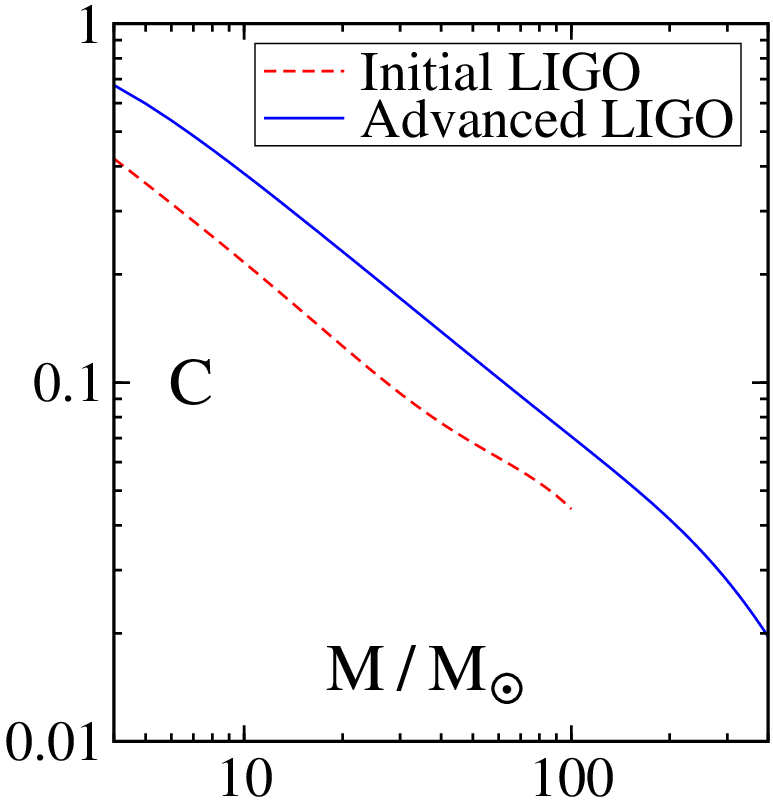
Figure 1 illustrates for non-spinning equal-mass binary black-hole waveforms (cf. Fig. 4 of Ref. [2]). This quantity can be evaluated in a straightforward way when any class of model waveforms is computed. The right side of Eq. (25) is always larger than the noise-weighted norm that appears on the left. Sufficient conditions for model-waveform accuracy based on the time-domain norm can be obtained therefore by replacing with the right side of Eq. (25) wherever it appears in the accuracy standards of Eqs. (13) and (14).
The norm of the waveform error caused by detector calibration errors, , is also difficult to evaluate because it depends on the gravitational waveform in addition to the purely detector-based errors and . The detector calibration-error terms in this norm can be isolated from the gravitational-waveform terms in a straightforward way using the inequality
| (28) | |||||
The right side of Eq. (28) is very easy to evaluate, and is always larger than the noise-weighted norm that appears on the left. Sufficient conditions for calibration accuracy based on can be obtained therefore by replacing with the right side of Eq. (28) wherever it appears in the accuracy standards of Eqs. (13) and (14).
In some circumstances the calibration-accuracy standards obtained using may be much stronger than necessary; for example when is sharply peaked at frequencies where the detector noise is large. In this case it may be advantageous to employ a different simplification of the accuracy standards. The detector calibration-error terms in the noise-weighted norm can also be isolated from the gravitational-waveform terms with an application of the Schwarz inequality:
| (29) |
This inequality can be re-written in the more compact form,
| (30) |
by defining a few useful quantities. The noise-weighted averages of and are defined as
| (31) | |||||
| (32) |
where the total detector noise, , is defined as
| (33) |
Note that the weight, , which appears in Eqs. (31) and (32) has integral one; so these are true (noise-weighted) averages of and . Note the unusual fourth power of the averaged quantity which appears in these definitions. This is required because that is the power of the error terms which appear on the right side of Eq. (29). Finally, the quantity that appears in Eq. (30) is the ratio of the standard signal-to-noise measure to another non-standard measure:
| (34) |
Figure 2 illustrates for non-spinning equal-mass binary black-hole waveforms using standard Initial and Advanced LIGO noise curves [5, 6]. This quantity can be evaluated in a straightforward way when any class of model waveforms is computed. It isn’t completely clear why the Advanced LIGO version of this curve is almost a factor of two smaller than the Initial LIGO curve. This may be due to the fact that the integral of in , Eq. (34), is dominated by its low frequency contributions where is largest. The Advanced LIGO noise curve is significantly smaller in this low-frequency range, so these contributions are much more significant in that case.
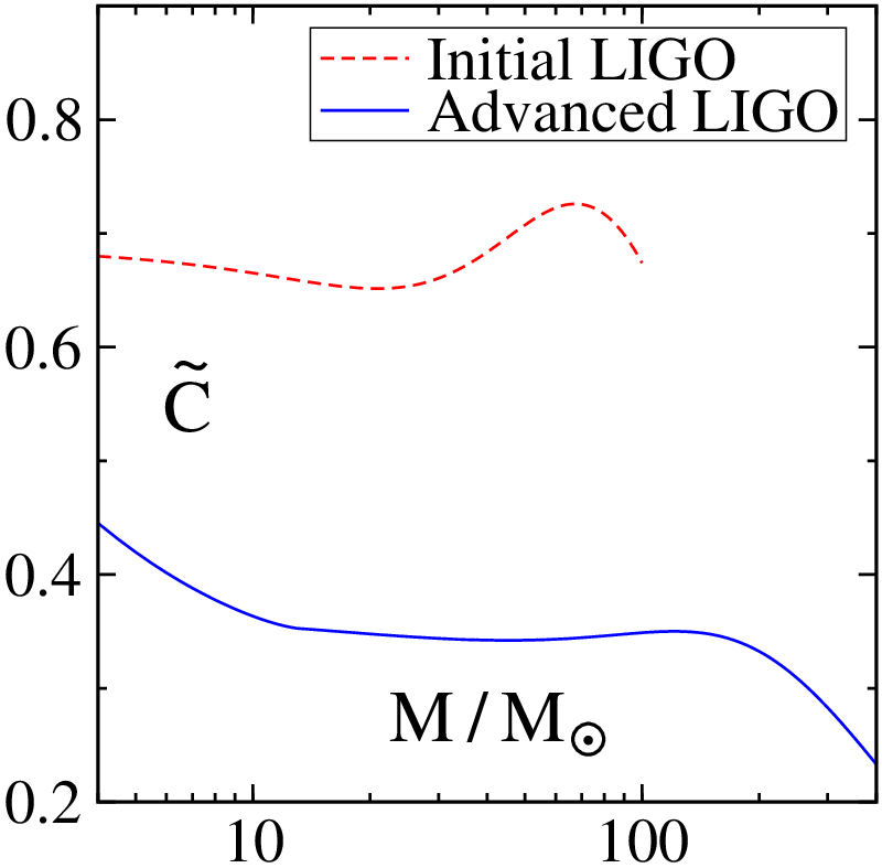
The maximum calibration-error, , and the noise-weighted averages, and , which appear in Eqs. (28) and (30) depend only on information that pertains to the detector itself. All of the dependence on the waveform in the original norm, , has been moved into the signal-to-noise ratio and the quantity . Thus the right sides of Eqs. (28) and (30) should be much easier for those performing detector calibrations to evaluate. The right sides of Eqs. (28) and (30) are always larger than the noise-weighted norm that appears on the left. Sufficient conditions for model-waveform accuracy based on the maximum calibration error (or the noise-weighted averages of the calibration errors and ) can be obtained therefore by replacing with the right side of Eq. (28) or (30) wherever it appears in the accuracy standards of Eqs. (13) and (14). The resulting accuracy standards based on the maximum calibration error [and using the re-written norm of the waveform-modeling error from Eq. (25)] become,
| (35) |
for measurement, and
| (36) |
for detection. Analogous versions of the standards based on the noise-weighted averages of the calibration errors, and , can be obtained in a similar way. Either version of the standards is sufficient to guarantee the needed level of accuracy for gravitational-wave data analysis. The most efficient choice for a particular detector, and for a particular type of source, will be determined by whether or is smaller.
IV Discussion
A new set of accuracy standards have been developed for the calibration and modeling errors of the waveforms used for gravitational-wave data analysis. The basic standards, Eqs. (13) and (14), are expressed most naturally in terms of the noise-weighted inner products commonly used in gravitational-wave data analysis. These basic expressions are not very convenient for actually applying the standards, however. So the basic standards have been transformed into expressions that are easier to apply: Eqs. (35) and (36). These new representations of the accuracy standards are slightly stronger, and if satisfied are sufficient to ensure the original standards are satisfied.
The new accuracy standards, Eqs. (35) and (36), prescribe a maximum for the combined calibration and modeling errors of the gravitational waveforms, not for each type of error separately. This means that an increased accuracy in one allows a somewhat weaker requirement on the other. Determining how to aportion the accuracy between the two error sources in an optimal way would require a careful analysis of the costs involved in reducing the error from each source. It seems reasonable to expect that requiring approximately equal accuracy for the calibration and modeling errors will be close to optimal. In this case the transformed expressions for the new accuracy requirements are
| (37) |
for measurement, and
| (38) |
for detection; the constant represents the signal-to-noise ratio of the strongest detected source. If the calibration of the instrument must be maintained at the level needed for accurate measurements of the strongest anticipated sources during the entire data collection period, then the accuracy requirements on the waveform-modeling error can be relaxed somewhat for detection:
| (39) |
These new accuracy standards should be applicable for essentially any gravitational-wave detector and any type of model waveform used in the data analysis process. To apply the standards for each particular case, the quantities , , and (perhaps) must be evaluated for the particular family of model waveforms, using the noise spectrum of the particular detector. Some insight can be gained into what the standards will actually look like by examining the case of binary black-hole inspiral-merger-ringdown waveforms using the Advanced LIGO noise curve. The quantities and have been computed for this case using an equal-mass non-spinning binary black-hole waveform obtained by matching together numerical and post-Newtonian waveforms [7, 8]. The results are depicted in Figs. 1 and 2 for binary systems with total masses in the range . From these graphs we see that and for these waveforms and the Advanced LIGO noise curve. The strongest binary black-hole signals in Advanced LIGO are expected to have signal-to-noise ratios that may be as large as . Assuming the template banks of model waveforms are constructed in the same way as those for Initial LIGO, the maximum mismatch compatible with a 10% event loss rate is . Substituting these values into the accuracy standards of Eqs. (37) and (38) results in the following calibration and waveform modeling accuracy requirements for Advanced LIGO:
| (40) |
for measurement, and
| (41) |
for detection. If the calibration accuracy is fixed at the higher level needed for measurements in the strongest sources for the entire period in which data is collected, then the standard on waveform-modeling error for detection can be relaxed to
| (42) |
A somewhat troubling feature of these conditions is the rather large coefficient that multiplies the norms of in these expressions. This is really just an artifact of the extremely long model waveform (containing about 1000 wave cycles) used here when evaluating [4]. The quantity contains the norm of the waveform in its denominator, and this norm becomes quite large when it is estimated using model waveforms with many wave cycles. This issue is discussed at some length in Ref. [4] and will not be addressed further here, since it does not bear directly on the main focus of this paper: deriving the optimal levels of calibration error.
Acknowledgements.
I thank Michael Landry for stimulating my interest in the questions addressed here and for comments and suggestions for improving an earlier draft of this paper. I also think Benjamin Owen and Yanbei Chen for several helpful discussions on these issues. This research was supported in part by a grant from the Sherman Fairchild Foundation, by NSF grants DMS-0553302, PHY-0601459, and PHY-0652995, and by NASA grant NNX09AF97G.References
- [1] A. Dietz, J. Garofoli, G. Gonzalez, M. Landry, B. O’Reilly, and M. Sung, Tech. Rep. LIGO-T050262-01-D, LIGO Project (2006), URL http://www.ligo.caltech.edu/docs/T/T050262-01.pdf.
- [2] L. Lindblom, B. J. Owen, and D. A. Brown, Phys. Rev. D 78, 124020 (2008).
- [3] S. Anderson et al., Tech. Rep. LIGO-T010095-00-Z, LIGO Project (2001), URL http://www.ligo.caltech.edu/docs/T/T010095-00.pdf.
- [4] L. Lindblom, Phys. Rev. D (2009), submitted, eprint arXiv:0907.0457.
- [5] A. Lazzarini and R. Weiss, LIGO science requirements document (1995), LIGO-E950018-02-E; See also, URL http://www.ligo.caltech.edu/~jzweizig/distribution/LSC_Data/.
- [6] GWINC: Gravitational Wave Interferometer Noise Calculator, v1 default parameters, URL http://lhocds.ligo-wa.caltech.edu:8000/advligo/GWINC.
- [7] M. A. Scheel, M. Boyle, T. Chu, L. E. Kidder, K. D. Matthews, and H. P. Pfeiffer, Phys. Rev. D 79, 024003 (2009).
- [8] M. Boyle, D. A. Brown, and L. Pekowsky, Comparison of high-accuracy numerical simulations of black-hole binaries with stationary-phase post-Newtonian template waveforms for Initial and Advanced LIGO, arXiv:0901.1628 (2009), eprint 0901.1628.