Kinetic energy density functionals from the Airy gas, with an application to
the atomization kinetic energies of molecules
Abstract
We construct and study several semilocal density functional approximations for the positive Kohn-Sham kinetic energy density. These functionals fit the kinetic energy density of the Airy gas and they can be accurate for integrated kinetic energies of atoms, molecules, jellium clusters and jellium surfaces. We find that these functionals are the most accurate ones for atomization kinetic energies of molecules and for fragmentation of jellium clusters. We also report that local and semilocal kinetic energy functionals can show ”binding” when the density of a spin unrestricted Kohn-Sham calculation is used.
pacs
71.15.Mb, 31.15.E-, 71.45.GmI Introduction
The positive Kohn-Sham (KS) [1] kinetic energy (KE) density of noninteracting electrons
| (1) |
is an exact functional of the occupied orbitals . Density functional approximations to the noninteracting kinetic energy can simplify and speed up by orders of magnitude any KS self-consistent calculation [2]. (Here and are the spin densities.) However, in spite of important and hard work done in this direction [3], no actual approximation has reached chemical accuracy.
The simplest model of an edge electron gas is the Airy gas, where any electron feels a linear effective potential [4], and thus the normalized one-particle eigenfunctions are proportional to the Airy function. The effective finite-linear-potential model gives remarkably good results for the jellium surface problem [5, 6]. However, the KE density derived in this approximation [7] does not recover the correct second-order gradient expansion KE density [8, 9] and has an unphysical oscillating behavior in the limit of slow density variations [10], being a poor approximation for atoms [11].
The positive KE density of the Airy gas was studied by Vitos et. al [12], and they derived a generalized gradient approximation (GGA) density functional for . (This approximation is denoted in this paper by VJKS GGA.) They showed that the poor behavior of the kinetic energy density derived in the linearized-potential approximation [7] is mainly due to a Laplacian term that arises naturally in the Airy gas model. Thus, the Laplacian term, even if it integrates to zero and does not affect the integrated KE, is an important tool in developing density functionals not only for the KE but also for the exchange-correlation (xc) energy [12, 13]. The VJKS GGA KE density functional fits the Airy gas KE density and is a good model for the KE density of the jellium surfaces, but for atoms and molecules it diverges to at the nuclei, due to the behavior of the Laplacian term. The integrated kinetic energies are at a Thomas-Fermi [14] level of accuracy, reducing considerably the error of the linearized-potential approximation [7].
A jellium surface is the simplest model of a metallic surface. Self-consistent local-spin-density (LSD) calculations [15] for this model provided early evidence that density functionals may work. But wavefunction-based methods, like Fermi hypernetted chain [16] and Diffusion Monte Carlo (DMC) of Ref. [17] predicted low-density surface xc energies about 40% larger than those from LSD. Recent refined DMC estimates [18], and calculations in the random phase approximation [19, 20] and beyond it [21, 22, 23], agree with the popular xc semilocal density functionals, showing that the jellium surface can not only be accurately described in the context of density functional theory, but can also be an important model used to develop new density functionals.
The exchange energy density of the Airy gas [4, 24, 25] and the xc jellium surface energies [25, 26] were employed in the construction of accurate xc GGA’s for solids. (See Refs. [24, 25, 26]). A simple xc GGA functional depends only on spin densities and their gradients and can not describe accurately both solids and atoms [27]. However, a Laplacian-level xc meta-GGA [13], that depends nontrivially on spin densities and their gradients and Laplacians, can be accurate for atoms, molecules, solids and surfaces.
In this paper, we derive several GGA KE functionals from the Airy gas and jellium surfaces and we find them accurate for atomization KE energies of molecules and for fragmentation of jellium clusters. Our functionals, constructed similarly to that of Ref. [12], recover the second-order gradient expansion of the integrated KE, have the right behavior of the KE density in the tail of the density, and fit the kinetic energy density of the Airy gas.
II Laplacian-dependent GGA kinetic energy functionals
The positive kinetic energy density of the local Airy gas (LAG) is [12]
| (2) |
where is the effective potential and is the density of the Airy gas. (Unless otherwise stated, atomic units are used throughout, i.e., .) Alternatively, Eq. (2) can be written [12] using the Thomas-Fermi kinetic energy density :
| (3) |
where
| (4) |
and is the slope of the linear effective potential. is a smooth function of the reduced density gradient
| (5) |
where is the Fermi wavevector. (The dimensionless density gradient measures the variation of the density over a Fermi wavelength .) Thus, Vitos et. al [12] proposed the following GGA KE density functional
| (6) |
where
| (7) |
fits for the Airy gas model. Eq. (6) recovers the exact KE density of the von Weizsäcker functional [28] for an exponentially decaying density (see Ref. [29]), but for a slowly-varying density behaves as and violates the second-order gradient expansion (GE2) of the KE density [8, 9]
| (8) |
Let us consider the following arbitrary partition of Eq. (3) for the Airy gas model
| (9) |
| (10) |
is a smooth function of the reduced gradient for any , and it can be accurately approximated by the following expression
| (11) |
where and are parameters that depend on . Eq. (11) recovers the terms for a slowly-varying density, but the second-order gradient expansion of the KE density additionally requires that . In the tail, where the density decays exponentially, Eqs. (9) and (11) give the correct KE density of the von Weizsäcker functional.
When , and we define a GGA (A) similar with the one in Ref. [12]
| (12) |
where the fitting parameters are shown in Table 1.
| A-GGA | A-GGA | A0.185-GGA | |
|---|---|---|---|
| 1.122609 | 1.301786 | 1.293576 | |
| 0.900085 | 3.715282 | 2.161116 | |
| -0.227373 | 0.343244 | -0.144896 | |
| 0.014177 | 0.032663 | 0.025505 | |
| 0.731298 | 2.393929 | 1.444659 |
When , we define a GGA (A) that recovers the second-order gradient expansion KE density
| (13) |
where the fitting parameters are shown in Table 1.
The Airy gas is the simplest edge electron gas and does not include curvature corrections that are present at the edge surfaces (see Fig. 2 of Ref. [4]). Thus in order to find an optimum value of for jellium surfaces, let us define the quality factor (similarly to Refs. [12] and [30])
| (14) |
where is an approximation of the positive Kohn-Sham KE density . [See Eq. (1)]. We apply the quality factor to jellium surfaces using numerical LSD Kohn-Sham orbitals and densities [15, 31]. The integration was done from to , where is the bulk Fermi wavelength , for several values of bulk parameter . (Here is the radius of a sphere which contains on average one electron, and is the bulk Fermi wavevector.) For we use Eqs. (9) and (11). Thus, for values of between 0.15 and 0.22, we accurately fit with the Padé approximation of Eq. (11), and we calculate . Fig. 1 shows that is minimum for for semi-infinite jellium surfaces with and .
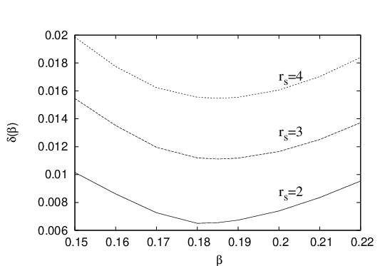
So from our jellium surface analysis we define the following GGA (A0.185) that also fits the kinetic energy density of the Airy gas
| (15) |
where the fitting parameters are shown in Table 1.
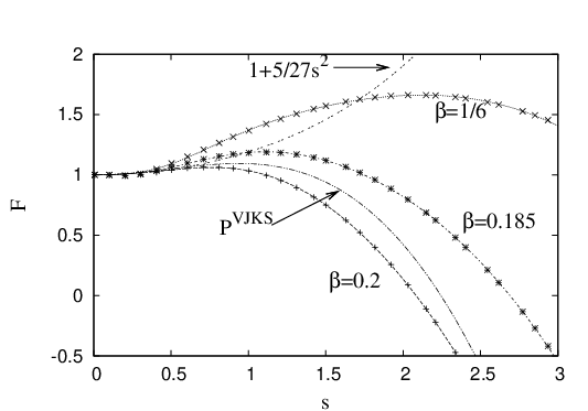
In Fig. 2 we show the exact function and the fitting function versus the scaled density gradient , for and 0.185 respectively. Up to , the exact functions and the parametrized ones can not be distinguished. (We note that values bigger than 3 are found in the tail of an atom or molecule, where the electron density is negligible.) overestimates until and underestimates for .
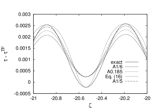
Far from the edge of the Airy gas, the density has Friedel oscillations [4]. These oscillations are well described by the kinetic energy density of the linear potential approximation [7] that in the slowly-varying density regime reduces to [10]
| (16) |
The third term represents quantum oscillations and has an unphysical behavior when . In Fig. 3 we show versus , for a slowly-varying Airy gas density. The edge is at . [ is the scaled spatial coordinate for the Airy gas.] The Friedel oscillations are well described by Eq. (16). But even if is the worst kinetic energy density shown in the figure, its integration over a period of the Friedel oscillations is almost exact. Thus , that behaves as in this limit, is the best approximation for the integrated KE, whereas gives the worst integrated KE.
III Tests of our GGA kinetic energy functionals
In this section we test our functionals for various systems. In the calculations we use the spin-scaling relation [32]
| (17) |
where is the density of the electrons with spin . ( or .)
III.1 Integrated kinetic energies of atoms, jellium clusters and jellium surfaces
In Table 2 we show the accuracy of , , , , , , and for atoms, jellium clusters and jellium surfaces (similarly as Table I of Ref. [13]). The error displayed in this table is
| (18) |
where “m.a.r.e. atoms” is the mean absolute relative error (m.a.r.e.) of the integrated kinetic energy of 50 atoms and ions (listed in Ref. [13]), “m.a.r.e. clusters” is the m.a.r.e. of , , , , , , , , and neutral spherical jellium clusters (with bulk parameter which corresponds to Na), and “m.a.r.e. LDM(N=8)” is the m.a.r.e. of the KE of N=8 jellium spheres for = 2, 4, and 6, calculated in the liquid drop model [13] (LDM)
| (19) |
where is the bulk Fermi wavevector, and is the surface KE. The exact LDM value is computed with the exact (using LSD orbitals). Because the relative errors of surface kinetic energies are much larger than those of the atoms and spherical jellium clusters, we use the LDM approach for calculating the jellium surface KE errors (as in Ref. [13]); LDM gives m.a.r.e. comparable to that of atoms and clusters (see Table 2). We use analytic Hartree-Fock densities and orbitals [33] for atoms and ions, and numerical Kohn-Sham densities and orbitals for jellium clusters (using the optimized potential method (OPM) [34]) and jellium semi-infinite surfaces (using LSD xc potential).
| m.a.r.e. | m.a.r.e. | m.a.r.e. | ||
| atoms | clusters | LDM(N=8) | Error (Eq. (18)) | |
| 0.0842 | 0.0439 | 0.0810 | 0.0733 | |
| 0.0399 | 0.0465 | 0.0754 | 0.0504 | |
| 0.0112 | 0.0099 | 0.0330 | 0.016 | |
| 0.0251 | 0.0176 | 0.0170 | 0.0212 | |
| 0.0626 | 0.0566 | 0.0879 | 0.067 | |
| 0.0789 | 0.0154 | 0.0177 | 0.048 | |
| 0.0083 | 0.0249 | 0.0535 | 0.024 |
, , and are constructed to model the KE density of the Airy gas, but only recovers the second-order gradient expansion of the KE density. The difference between and is given mainly by the quality of fitting the function of Eq. (4). (See Fig. 2.) includes effects of density variations near jellium surfaces because of our optimization of the Laplacian coefficient. In Table 2 we see that is very accurate (comparable with the fourth-order gradient expansion) for jellium systems and gives an overall error smaller than and . is accurate for atoms and gives an overall error comparable with the fourth-order gradient expansion one ( see also Table 1 of Ref. [13]).
III.2 Integrated atomization kinetic energy for a set of molecules
In Table 3 we present the atomization kinetic energies for the molecules used in Refs. [13, 35]. We observe that keeps the right sign for all the molecules and has practically the same mean absolute error as the Thomas-Fermi functional. In Ref. [35] it was shown that the Thomas-Fermi KE functional gives better atomization kinetic energies than all the other tested semilocal functionals. is accurate for atoms and molecules, and gives the smallest mean absolute error for the atomization energies presented in Table 3. We also show that the PBE-like semilocal functional of Ref. [38], whose parameters are fitted to atoms, works worse than the Thomas-Fermi functional and all the semilocal functionals derived from the Airy gas.
| -0.150 | -0.097 | -0.086 | -0.114 | -0.080 | -0.114 | -0.096 | -0.108 | |
| -0.185 | -0.305 | -0.369 | -0.186 | -0.422 | -0.173 | -0.311 | -0.226 | |
| -0.304 | -0.308 | -0.455 | -0.136 | -0.531 | -0.169 | -0.369 | -0.209 | |
| -0.601 | -0.737 | -0.907 | -0.571 | -0.972 | -0.618 | -0.813 | -0.649 | |
| -0.397 | -0.231 | -0.457 | -0.060 | -0.525 | -0.165 | -0.364 | -0.155 | |
| -0.298 | -0.323 | -0.580 | -0.085 | -0.678 | -0.181 | -0.456 | -0.203 | |
| -0.053 | 0.128 | 0.013 | 0.282 | -0.050 | 0.269 | 0.093 | 0.223 | |
| -0.340 | -0.1835 | -0.539 | 0.079 | -0.644 | -0.097 | -0.399 | -0.071 | |
| -0.158 | 0.344 | -0.046 | 0.565 | -0.134 | 0.321 | 0.069 | 0.412 | |
| -0.431 | -0.215 | -0.539 | 0.005 | -0.631 | -0.168 | -0.424 | -0.129 | |
| -0.268 | 0.092 | -0.215 | 0.330 | -0.313 | 0.176 | -0.094 | 0.198 | |
| -0.100 | 0.106 | -0.089 | 0.335 | -0.177 | 0.286 | 0.030 | 0.239 | |
| m.a.e. | 0.177 | 0.133 | 0.311 | 0.172 | 0.224 | 0.116 | 0.232 |
III.3 Binding energy of the molecule
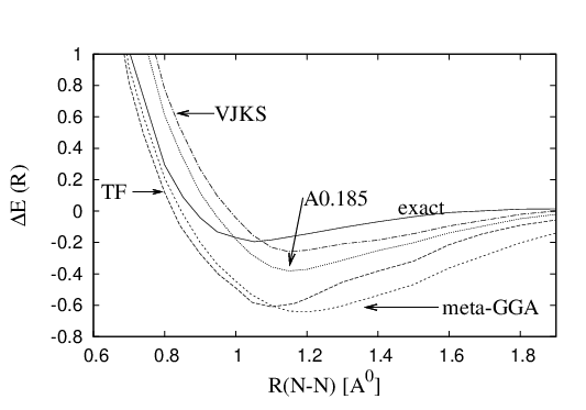
In Fig. 4 we show the binding energy of the molecule as a function of the distance between the nuclei. We use a spin unrestricted Hartree-Fock calculation in which the spin symmetry breaks close to the Hartree-Fock equilibrium bond length. This helps the functionals to show an equilibrium length close to the exact. Figure 4 is in accord with the values for the molecule listed in Table 3; all the semilocal functionals presented in the figure give bigger atomization kinetic energies than the exact calculation, thus showing a minimum in the total energy calculated with the Hartree-Fock density.
The unrestricted solution becomes energetically lower beyond the Coulson-Fisher point [39] than the energy of the restricted solution, and spin symmetry breaking for the molecule can be achieved by mixing the highest occupied and lowest unoccupied orbitals [40]. For a spin-restricted calculation, the orbital-free KE functionals listed in Table II do not show an equilibrium point, thus the spin-breaking symmetry [41, 42, 43] and the spin-scaling relations [32] play an important role in describing stretched molecules, and they need to be taken into account in the orbital-free codes.
III.4 Tests of the kinetic energy density
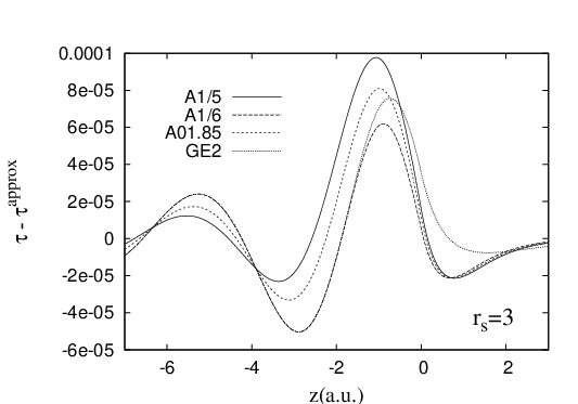
In Fig. 5 we show the kinetic energy density of our functionals at a jellium surface. Though has the smallest overall error, gives the most accurate surface kinetic energy because it is accurate near the surface and it can almost exactly damp the Friedel oscillations far from the surface (see Fig. 3).
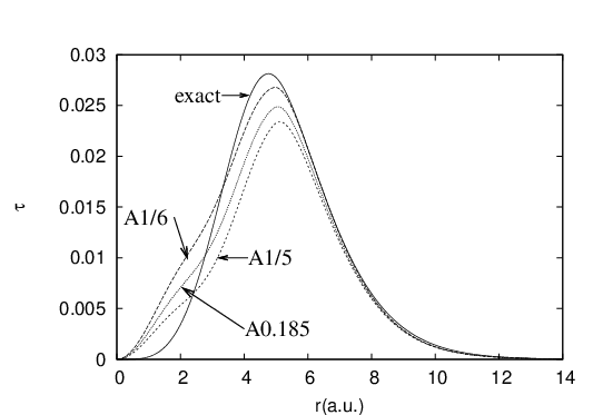
In Fig. 6 we show the kinetic energy densities of our functionals for the Na jellium cluster. Here the exact curve is the von Weizsäcker [28] KE density. We see that all three functionals (, , and ) recover the exact curve in the tail of the density, as expected.
III.5 Large- asymptotic behavior
The non-interacting kinetic energy of the neutral atoms has the following asymptotic expansion [44, 45]:
| (20) |
where is the atomic number, and , , and . In Ref. [45] the authors propose an accurate method to extract these coefficients for any KE functional. In Table 4 we present the large- asymptotic behavior of our functionals. All the functionals listed in Table 4 are exact for systems with uniform density, such that we expect that they have the exact Thomas-Fermi coefficient . (Similarly with Ref. [45], we do not have enough data points to extract accurately.) and , the functionals that give the most accurate atomization kinetic energies, have reasonable large- asymptotic behaviors.
| Exact | 0.768745 | -0.500000 | 0.269900 |
|---|---|---|---|
| 0.768745 | -0.536197 | 0.335992 | |
| 0.768745 | -0.507979 | 0.291815 | |
| 0.768745 | -0.532065 | 0.229370 | |
| 0.768745 | -0.439745 | 0.392152 | |
| 0.768745 | -0.491080 | 0.302999 | |
| 0.768745 | -0.507589 | 0.225358 |
III.6 Fragmentation of jellium clusters
Let us consider the disintegration of the neutral spherical jellium Na cluster into smaller closed-shell jellium spheres:
| (21) |
where are positive integers, and . We define the disintegration KE as
| (22) |
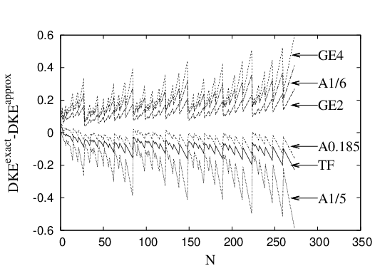
In Fig. 7 we show for 273 processes described by Eq. (21), for several KE functionals. We see that our functional is very accurate, improving over for all the configurations. is close to, but better than the fourth-order gradient expansion . Overall, this figure agrees well with the atomization KE of molecules reported in Table 3, showing an important link between jellium spheres and molecules. These results and the liquid drop model (see Eq. (17) of Ref.[45]) suggest that the TF functional gives a good balance between jellium surface KE and jellium curvature KE. This balance, that is important in atomization and disintegration processes, is improved by the A0.185-GGA functional.
IV Conclusions
In this paper we have studied several semilocal KE density functionals derived from the Airy gas. These functionals, that depend trivially on the Laplacian of the density, do not satisfy several important constraints. Their kinetic energy densities are not always positive, and they implicitly violate the important constraint (here is the von Weizsäcker KE density) and diverge to at the nucleus of an atom.
However, such functionals can be accurate for the integrated KE of jellium surfaces and jellium clusters (e.g. ), and of atoms and molecules (e.g. ), when we use realistic densities ( from KS calculations). More importantly, they are the most accurate KE density functionals, to our knowledge, for the integrated atomization kinetic energies of molecules and for the fragmentation of jellium clusters. These functionals may also be useful for quasi-realistic densities (e.g. a superposition of free-atom Kohn-Sham densities), but they are not accurate enough for orbital-free calculations.
We have also presented a spin-unrestricted Hartree-Fock calculation for the stretched molecule that explains the atomization kinetic energies displayed in Table 3, and that shows equilibrium lengths for many semilocal functionals. Thus, this work suggests that the spin-symmetry breaking and the spin scaling relations can be important tools in orbital-free approaches.
Acknowledgments: We thank Professor John P. Perdew for many valuable discussions and suggestions. L.A.C. acknowledges NSF support (Grant No. DMR05-01588).
References
- [1] W. Kohn and L.J. Sham, Phys. Rev. , A1133 (1965).
- [2] An orbital-free kinetic energy density functional can be used in solving the spin-dependent Euler equations, or perhaps applied to a superposition of atomic Kohn-Sham or Hartree-Fock densities.
- [3] ”Recent advances in developing orbital-free kinetic energy functionals”, V.V. Karasiev, R.S. Jones, S.B. Trickey, and F.E. Harris, in New Developments in Quantum Chemistry, J.P. Paz and A.J. Hernández eds. (Research Signposts), in press.
- [4] W. Kohn and A.E. Mattsson, Phys. Rev. Lett. , 3487 (1998).
- [5] V. Sahni, C.Q. Ma, and J.S. Flamholz, Phys. Rev. B , 3931 (1978).
- [6] A. Solomatin and V. Sahni, Phys. Rev. B , 3655 (1997).
- [7] R. Baltin, Z. Naturforsch. Teil A , 1176 (1972).
- [8] D.A. Kirzhnitz, Sov. Phys. JETP , 64 (1957), D.A. Kirzhnitz, “Field Theoretical Methods in Many-Body Systems”, Pergamon, Oxford, 1967.
- [9] M. Brack, B.K. Jennings and Y.H. Chu, Phys. Lett. , 1 (1976).
- [10] R.M. Dreizler and E.K.U. Gross, “Density Functional Theory”, Springer-Verlag (1990).
- [11] S.K. Ghosh and L.C. Balbas, J. Chem. Phys. , 5778 (1985).
- [12] L. Vitos, B. Johansson, J. Kollár, and H. L. Skriver, Phys. Rev. A , 052511 (2000).
- [13] J.P. Perdew and L.A. Constantin, Phys. Rev. B , 155109 (2007).
- [14] L.H. Thomas, Proc. Cambridge Phil. Soc. , 542 (1926), E. Fermi, Rend. Accad. Naz. Lizei , 602 (1927).
- [15] N.D. Lang and W. Kohn, Phys. Rev. B , 4555 (1970).
- [16] E. Krotscheck and W. Kohn, Phys. Rev. Lett. , 862 (1986).
- [17] P.H. Acioli and D.M. Ceperley, Phys. Rev. B , 17199 (1996).
- [18] B. Wood, N.D.M. Hine, W.M.C. Foulkes, and P. García-González, Phys. Rev. B , 035403 (2007).
- [19] J.M. Pitarke and A.G. Eguiluz, Phys. Rev. B , 045116 (2001).
- [20] J.M. Pitarke, L.A. Constantin, and J.P. Perdew, Phys. Rev. B , 045121 (2006).
- [21] J. M. Pitarke and J. P. Perdew, Phys. Rev. B , 045101 (2003).
- [22] L.A. Constantin, J.M. Pitarke, J.F. Dobson, A. Garcia-Lekue, and J.P. Perdew, Phys. Rev. Lett. , 036401 (2008)
- [23] L.A. Constantin, J.P. Perdew, and J. Tao, Phys. Rev. B , 205104 (2006)
- [24] L. Vitos, B. Johansson, J. Kollár, and H. L. Skriver, Phys. Rev. B , 10046 (2000)
- [25] R. Armiento and A.E. Mattsson, Phys. Rev. B , 085108 (2005).
- [26] J.P. Perdew, A. Ruzsinszky, G.I. Csonka, O.A. Vydrov, G.E. Scuseria, L.A. Constantin, X. Zhou, and K. Burke, Phys. Rev. Lett. , 136406 (2008).
- [27] J.P. Perdew, L.A. Constantin, E. Sagvolden, and K. Burke, Phys. Rev. Lett. , 223002 (2006).
- [28] C.F. von Weizsäcker, Z. Phys. , 431 (1935).
- [29] In the tail of a spherical atom, the density decays exponentially as , so when , and in this asymptotic region.
- [30] D. García-Aldea and J.E. Alvarellos, J. Chem. Phys. , 074103 (2008).
- [31] R. Monnier and J.P. Perdew, Phys. Rev. B , 2595 (1978).
- [32] G.L. Oliver and J.P. Perdew, Phys. Rev. A , 397 (1979).
- [33] E. Clementi and C. Roetti, Atomic Data Nucl. Data Tables , 177 (1974).
- [34] S. Kümmel and John P. Perdew, Phys. Rev. Lett. , 043004 (2003), and references therein.
- [35] S.S. Iyengar, M. Ernzerhof, S.N. Maximoff and G.E. Scuseria, Phys. Rev. A , 052508 (2001).
- [36] A.D. Becke, Phys. Rev. A , 3098 (1988).
- [37] J.P. Perdew, in Electronic Structure of Solids ‘91, edited by P. Ziesche and H. Eschrig (Akademie Verlag, Berlin, 1991).
- [38] F. Tran and T.A. Wesolowski, Int. J. Quantum Chem. , 441 (2002).
- [39] M. Fuchs, Y.-M. Niquet, X. Gonze, and K. Burke, J. Chem. Phys. , 094116 (2005), and references therein.
- [40] A.M. Lee and N.C. Handy, J. Chem. Soc. Faraday Trans. , 3999 (1993).
- [41] O. Gunnarsson and B.I. Lundqvist, Phys. Rev. B , 4274 (1976).
- [42] J.P. Perdew, A. Savin, and K. Burke, Phys. Rev. A , 4531 (1995).
- [43] J.A. Pople, P.M.W. Gill, and N.C. Handy, Int. J. Quantum Chem. , 303 (1995).
- [44] B.-G. Englert, Semiclassical Theory of Atoms, (Lecture Notes in Physics, Springer-Verlag, Berlin, 1988), and references therein.
- [45] D. Lee, K. Burke, L.A. Constantin, and J.P. Perdew, J. Chem. Phys., accepted for publication.