Exchange-Correlation Energy Functional Based on the Airy-Gas Reference System
Abstract
In recent work, generalized gradient approximations (GGA’s) have been constructed from the energy density of the Airy gas for exchange but not for correlation. We report the random phase approximation (RPA) conventional correlation energy density of the Airy gas, the simplest edge electron gas, in which the auxiliary noninteracting electrons experience a linear potential. By fitting the Airy-gas RPA exchange-correlation energy density and making an accurate short-range correction to RPA, we propose a simple beyond-RPA GGA density functional (”ARPA+”) for the exchange-correlation energy. Our functional, tested for jellium surfaces, atoms, molecules and solids, improves mildly over the local spin density approximation for atomization energies and lattice constants without much worsening the already-good surface exchange-correlation energies.
pacs
71.10.Ca,71.15.Mb,71.45.GmI Introduction
In Kohn-Sham density functional theory [1], the ground-state density and energy of interacting electrons in a scalar external potential are computed efficiently via a selfconsistent calculation for an auxiliary system of noninteracting electrons in a scalar effective potential . Once the exchange-correlation energy as a functional of the electron density has been approximated, its functional derivative provides the exchange-correlation contribution to . By itself, the deviation of from the constant chemical potential determines the electron density and thus the correlation energy. Typical approximations are designed to be exact for a reference system, most often the uniform electron gas in which the auxiliary noninteracting electrons see a constant or uniform . Sometimes additional exact constraints or fits to experiment are also built into the approximation. Recently Kohn and Mattsson [2] have proposed as a more realistic reference system the edge electron gas, in which varies more or less linearly near the edge surface of the density. While the uniform gas could be (and is) a good reference for a bulk solid, the edge electron gas could be at least as good for a bulk solid and better for solid surfaces, molecules, and atoms, which have regions where the electron density evanesces.
The edge surface of any electron system is defined [2] by , where is the exact Kohn-Sham [1] (KS) effective potential and is the chemical potential. Outside this classical turning surface, all noninteracting electrons tunnel into a barrier. The simplest example of an edge electron gas is the Airy gas, where any electron feels a linear effective potential [2], and thus the normalized one-particle eigenfunctions are proportional to the Airy function. The Airy gas has not only a surface-like region, but also a region of high and slowly-varying (Thomas-Fermi-like) electron density where the local density approximation (with uniform-gas input) is accurate [2, 3] for the noninteracting kinetic, exchange, and correlation energy densities.
The Airy gas has appeared before in density functional theory: (1) The effective finite-linear-potential model gives remarkably good results for the jellium surface problem, where the orbitals of this model are approximated with plane waves inside the bulk, Airy functions near the surface, and exponential functions far in the vacuum [4, 5, 6]. (2) Baltin [7] constructed a generalized gradient approximation (GGA) for the orbital kinetic energy from the Airy-gas kinetic energy density, but his approximation does not recover the second-order gradient expansion for the kinetic energy density [8, 9] and is poor for atoms and molecules [10, 11]. However, the kinetic energy density of the Airy gas [11] can still be a starting point for construction of GGA kinetic energy functionals that can be more accurate for atoms, molecules, jellium clusters, and jellium surfaces [11, 12]. The trick is to fit a GGA plus a term integrating to zero to the Airy-gas kinetic energy density.
The exchange energy density of the Airy gas [2] was fitted [13, 14] with a function dependent on the density and its gradient. Thus, Vitos et. al [13] developed a GGA exchange energy functional (LAG or local Airy-gas GGA) that was used with the local spin-density approximation (LSDA) correlation energy. This exchange-correlation (xc) energy functional gives results for atoms very close to, but better than, the LSDA ones, and its accuracy for atomization energy of diatomic molecules is similar to that of the PBE GGA [15], while for bulk systems the results of LAG GGA are close to the PBEsol GGA [16] and to experimental values. However, the jellium xc surface energies of LAG are far too low (lower even than those of the PBE GGA). Armiento and Mattsson [14, 17] proposed an xc energy functional (AM05 GGA) using a better fit for the Airy gas exchange energy density and a correlation energy functional constructed such that the AM05 xc jellium surface energies fit the RPA+ [18] values (RPA plus a GGA short-range correction). AM05 is also based on the subsystem functional approach [19], which permits an interpolation between a uniform-gas reference for the bulk of a solid and an Airy-gas reference for the surface. (Since the Airy-gas reference system by itself provides such an interpolation, we make no further interpolation here.) AM05 slightly improves the accuracy of LAG GGA for bulk systems.
Because the correlation energy density of the Airy gas was unknown, the LAG GGA and AM05 GGA used in their construction only the Airy-gas exchange energy density. In this paper we compute the correlation energy density of the Airy gas in the random phase approximation (RPA), and fit it to a GGA (ARPA). As in Refs. [13] and [14], our fit is made without regard to exact constraints on . The Airy gas is a system of delocalized electrons where the self-interaction correction has no effect, and where the GGA correction [18] to the integrated RPA energy should be accurate. Our functional, including this GGA correction to RPA, will be called ARPA+.
Unlike energies, energy densities of non-uniform systems are not unique. It is not clear to us that the conventional choice for the exchange-correlation energy density (made in Refs. [13, 14], and here) is optimal. It is not our intention here to either endorse or criticize this choice, but simply to see what GGA is obtained from the Airy-gas reference system within a consistent implementation for correlation as well as exchange.
AM05, PBEsol, and ARPA+ are of special interest as candidates for a ”GGA for solids” providing better lattice constants and surface energies than standard GGA’s like PBE, possibly at the cost of a worsened description of atoms and molecules. There have been several recent articles commenting on or testing for solids the LAG, AM05, and PBEsol GGA’s [20, 21, 22, 23, 24].
Our paper is organized as follows. In section II, we propose a simple model for the Airy gas. In section III, we construct the ARPA+ GGA xc energy functional from our Airy gas model. In section IV we test the ARPA+ GGA for atoms, molecules, jellium surfaces and bulk solids. In section V, we summarize our conclusions.
II The Airy gas model
The simplest example of an edge electron gas is the Airy gas that is translationally invariant in the plane of the surface () and has the effective potential [2, 25]
| (1) |
Here is the slope of the effective potential and the characteristic length scale
| (2) |
is approximately the edge region thickness [2]. (Unless otherwise stated, atomic units are used throughout, i.e., .)
The KS orbitals are , where and are the wavevector and the position vector parallel to the plane of the surface, is the cross-sectional area, and the orthonormal eigenfunctions satisfy the equation
| (3) |
with the boundary conditions
| (4) |
They are given by the Airy functions
| (5) |
where is the Airy gas characteristic energy scale, is the normalization constant, and is the -th eigenvalue calculated from the boundary condition . The Airy gas density is
| (6) |
We recall that all 3D states with energy up to are occupied. Thus the Airy gas is completely determined by the length and the energy .
In the limit , the normalization constant is [2]
| (7) |
and the eigenvalues are [2]
| (8) |
So, the density of the Airy gas is
| (9) |
where
| (10) |
Let us consider a model for the Airy gas that is described by Eqs. (1) - (6), but instead of choosing we take for computational convenience. Such a system has 19 occupied orbitals and can accurately describe the Airy gas. The normalization constants of Eq. (5) and the eigenvalues are computed numerically. Such an approach is similar to jellium slabs that are described by a finite number of occupied orbitals in the -direction and that can accurately predict the surface energies of semi-infinite jellium surfaces [26].
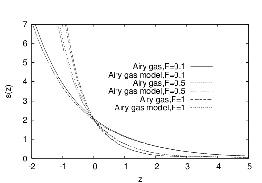
We select three values , , and for the slope of the effective potential. The accuracy of the model does not depend on the value. In Fig. 1 we show the densities of the Airy gas and of our Airy gas model for the chosen values of the slope . We see the exact Airy gas densities and the modeled ones can not be distinguished until where the densities of our model have oscillations until they vanish.

Important ingredients of any GGA functional are the density and the reduced density gradient
| (11) |
where is the Fermi wavevector. (The dimensionless density gradient measures the variation of the density over a Fermi wavelength .) In Fig. 2 we compare the reduced gradients of our model and of the exact Airy gas. Up to , the model nicely matches the exact Airy gas, and it is accurate for any value of . (We note that values bigger than 3 are found in the tail of an atom or molecule, where the electron density is negligible. We also note that in most bulk solids the maximum [24] value of the reduced gradient is smaller than 2.)
III RPA correlation energy density of the Airy gas, and the construction of the ARPA+ GGA
The conventional xc energy density at a point is , where is the local electron density and is the conventional xc energy per particle. Let us consider the spin-unpolarized Airy gas model with the edge plane at . Using its translational invariance in a plane perpendicular to the axis, and the so-called adiabatic-connection fluctuation-dissipation theorem [27, 28, 29, 26] (ACFDT), the exact expression for the conventional xc energy per particle at point is [27, 28, 26]
| (12) |
where is the wavevector parallel to the surface, and and are the two-dimensional Fourier transforms of the interacting density response function at the coupling strength and of the Coulomb potential respectively. The substitution of with the non-interacting density response function into Eq.(12) yields the exact (expressible in terms of occupied orbitals only, although requires also the unoccupied orbitals). The density response function obeys the screening integral Dyson-like equation [30]
| (13) |
where and is the exact xc kernel. Here is the exact frequency-dependent xc potential at coupling strength . Obviously, the exact xc kernel is unknown and it has to be approximated. Approximations of the xc kernel are usually constructed from the uniform electron gas [31, 32, 33], and have not been tested sufficiently for nonuniform systems. When is taken to be zero, Eq. (13) reduces to the RPA. The RPA xc hole density is exact at large interelectronic separations such that it can correctly describe the xc hole density of an electron far outside of a jellium surface [34], and its on-top hole is finite and well described by the LSDA-RPA [18] on-top hole in the case of a jellium surface [34].
Eqs. (12) and (13) can be generalized [35] for systems with any relative spin polarization
| (14) |
where and are the spin densities, . Thus for the Airy gas model, we choose to calculate the RPA correlation energy per particle at point z, from Eqs. (12) and (13), and to add the RPA+ short-range correction:
| (15) |
where is the PBE GGA [15] xc energy, and is the PBE-RPA GGA xc energy [18]. The exchange contribution and the long-range correlation contribution cancel out of the bracketed term in Eq. (15), leaving only short-range correlation. Because the self-interaction correction is not important for the Airy gas, Eq. (15) will give nearly the exact correlation energy of the Airy gas.
For the numerical evaluation of Eqs. (12) and (13), we follow the method described in Refs. [26] and [36], but instead of using the double- and single-cosine representations of the density response function and the density respectively, we use a grid on the -axis for and . We find that the first 50 unoccupied orbitals are enough for an accurate calculation. (Our grid on the -axis can accurately describe the occupied and the first 50 unoccupied orbitals [37]).
The exchange energy for a spin-polarized system may be evaluated from the spin-unpolarized version using the spin-scaling relation [38]:
| (16) |
and thus we only need to consider the spin-unpolarized case. We fit the exchange energy per particle of the Airy gas model, using the non-linear least-square Levenberg-Marquardt method [39], with the following expression
| (17) |
where and the enhancement factor is
| (18) |
where , , , are the parameters found in Ref.[13], and , , , , , are parameters found from our fitting procedure. Eq. (17) recovers the correct LSDA for the uniform electron gas, and fits well the Airy gas exchange energy per particle for . ( Values of bigger than 20 are found only when the density is negligible. We recall that LAA of Ref. [14] is a better fit than LAG or far outside the edge.)
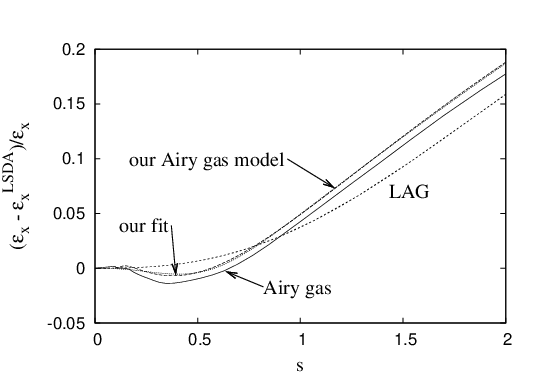
In Fig. 3 we show versus the reduced gradient for several approximations. The Airy gas curve, as well as our Airy gas model curve, have a negative region around that was not taken into account by the LAG GGA and AM05 GGA. We find this fine feature only because we plot instead of . (This feature can also be seen in the inset of Fig. 1 of Ref. [14], but it was not taken into account in the construction of AM05.) The second term of the right-hand-side of Eq. (18) models the exact behavior at small reduced gradients, whereas the first term of the right-hand-side of Eq. (18) has the same form as the parametrization proposed in Ref. [13]. We observe that our fit (Eqs. (17) and (18)) is very close to the exact Airy gas model as well as to the exact Airy gas exchange energy per particle.
We fit the RPA correlation energy per particle of the Airy gas of any spin polarization with the following expression, using again the non-linear least-square Levenberg-Marquardt method [39]
| (19) |
where is the local Wigner-Seitz radius [], is the relative spin polarization of Eq. (14), is the RPA correlation energy per particle of the uniform electron gas (see Ref. [40]), and
| (20) |
with being a spin-scaling factor. The correlation enhancement factor is
| (21) |
with , , , and . Eq. (21) is a simple Padé approximation that recovers the RPA behavior of the uniform electron gas when . All the parameters were found by the fitting procedure, and not by constraints on the integrated correlation energy (which would suggest [15] an exponent of 7/6 and the appearance of in the denominator of Eq. (20), and a quadratic term in the small-gradient expansion of Eq. (21)). The irrelevance of some standard constraints may be related to the absence [41] of a second-order gradient expansion for the conventional correlation energy density. Given , is a function of , and is a monotonic (hence invertible) function of , so can be expressed as a function of . Since there is a one-to-one correspondence between the and our , we can do the fitting. The fitting was done for between 0 and 20.
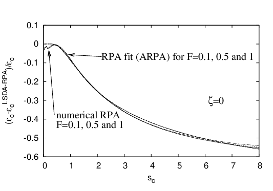

In Figs. 4 and 5 we show versus for the spin-unpolarized Airy gas model () and fully-spin-polarized Airy gas model () respectively, for the slopes of the the effective potential used in Figs. 1 and 2 (, 0.5, and 1). We note that our numerical calculation is accurate for , see Ref. [37]. We see in both figures that the numerical RPA correlation energy density does not depend much on the slope value when they are plotted against , motivating our definition of in Eq. (20) and making the fit of the RPA correlation energy per particle independent of the value [42] (see Eqs. (19) and (21)). For the ARPA of Eq. (19) is close to exact even if it does not match well the detailed exact behavior, as it does in the region .
Overall we consider
| (22) |
an xc GGA functional that fits very well the Airy gas RPA xc energy density. Thus making the RPA+ short-range correction (see Eq. (15)) to ARPA GGA, we propose the following GGA xc functional (ARPA+ GGA) constructed from the Airy gas
| (23) |
The nonlocality of a GGA is displayed by the enhancement factor [43, 44]
| (24) |
being the exchange energy per particle of a spin-unpolarized uniform electron gas. For a spin-unpolarized system in the high-density limit (), the exchange energy is dominant and Eq. (24) defines the exchange enhancement factor .
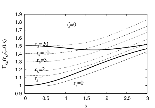
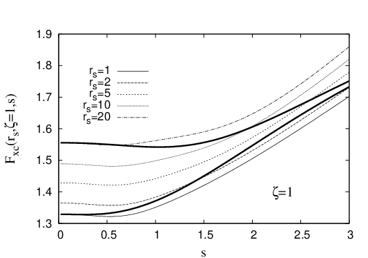
Figs. 6 and 7 show the enhancement factor of ARPA+ compared to PBEsol as a function of the reduced gradient , for several values of , in the spin-unpolarized case and the fully-spin-polarized case, respectively. In both figures, the ARPA+ and PBEsol enhancement factors agree well at small gradients (for ), but for ARPA+ shows more exchange-correlation nonlocality than PBEsol.


Figs. 8 and 9 show a comparison between the ARPA+ GGA and AM05 GGA enhancement factors, for the spin-unpolarized and fully spin-polarized cases. Up to , and agree very well. For , shows slightly more nonlocality than , and, even if this difference is small, it has noticeable effects for the lattice constants of bulk solids. Overall, our ARPA+ confirms the AM05 construction for correlation.
IV Tests of the ARPA+ GGA xc energy functional
In this section we test our functionals for jellium surfaces, atoms, molecules, and bulk solids. The calculations use the spin-scaling relation of Eq. (16).
IV.1 Jellium surfaces
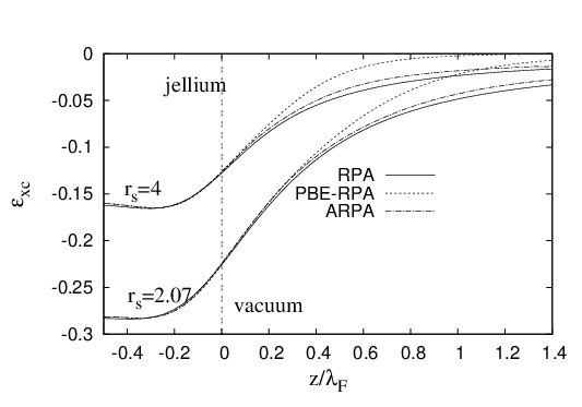
In Fig. 10 we show given by Eq. (12), given by Eq. (22), and of Ref. [18], for two thick jellium slabs of bulk parameters and . We use accurate LSDA orbitals and densities as in Refs. [26, 45, 46]. ARPA fits well the exact RPA until , showing that the Airy gas and the jellium surfaces are very close related, as expected.
In Table 1 we report the ARPA and ARPA+ jellium surface exchange and xc energies. The are close to but worse than . The are between and for , but lower than both others for . The are reasonably close to and (see Ref. [48]), but are surprisingly lower and less accurate than .
| 2 | 3 | 4 | 6 | |
| 3036 | 669 | 222 | 43.6 | |
| 2436 | 465 | 128 | 11.8 | |
| 2666 | 540 | 162 | 22.9 | |
| 2553 | 498 | 141 | 15.4 | |
| 2908 | 619 | 198 | 34.3 | |
| 2896 | 615 | 196 | 33.6 | |
| 2934 | 627 | 201 | 35.4 | |
| 2941 | 626 | 199 | 34.6 | |
| 2624 | 526 | 157 | 22 | |
| 3403 | 781 | 269 | 56 | |
| 3318 | 760 | 262 | 55 | |
| 3366 | 764 | 260 | 53 | |
| 3467 | 801 | 278 | 58 | |
| 3354 | 764 | 261 | 53 | |
| 3265 | 741 | 252 | 52 | |
| 3374 | 774 | 267 | 56 | |
| 3380 | 772 | 266 | 55 | |
| 3226 | 714 | 237 | 43.7 | |
| 3414 | 782 | 270 | 56.7 | |
| 3313 | 745 | 250 | 50 | |
| 3413 | 781 | 268 | 54 | |
| 3392 | 768 | 261 | 52.5 … |
IV.2 Spherical atoms
In Table 2 we calculate the ARPA+ exchange and correlation energies of several atoms and ions. We use spin-restricted analytic Hartree-Fock orbitals [51] and densities. (The difference between Hartree-Fock orbitals and Kohn-Sham orbitals is small for atoms.) For every atom and ion of Table 2, ARPA+ GGA improves the LSDA results, but it is still a poor approximation in comparison with GGA’s constructed for atoms and molecules, such as PBE GGA [15, 3].
| H | -0.268 | -0.280 | -0.313 | -0.0222 | -0.0199 | 0 |
|---|---|---|---|---|---|---|
| He | -0.884 | -0.925 | -1.026 | -0.1125 | -0.1030 | -0.0420 |
| -1.421 | -1.486 | -1.652 | -0.1346 | -0.1233 | -0.0435 | |
| -1.957 | -2.047 | -2.277 | -0.1504 | -0.1378 | -0.0443 | |
| Li | -1.538 | -1.603 | -1.781 | -0.1508 | -0.1378 | -0.0453 |
| -2.168 | -2.261 | -2.507 | -0.1727 | -0.1578 | -0.0474 | |
| Be | -2.312 | -2.408 | -2.667 | -0.2240 | -0.2058 | -0.0943 |
| -3.036 | -3.157 | -3.492 | -0.2520 | -0.2317 | -0.1113 | |
| -6.634 | -6.886 | -7.594 | -0.3336 | -0.3069 | -0.1799 | |
| N | -5.893 | -6.047 | -6.596 | -0.4273 | -0.4016 | -0.1883 |
| Ne | -11.033 | -11.220 | -12.109 | -0.7428 | -0.7084 | -0.3905 |
| Ar | -27.863 | -28.118 | -30.190 | -1.4242 | -1.3723 | -0.7222 |
| m.a.e. | 0.600 | 0.481 | 0.1865 | 0.1664 |
| Li | -0.133 | -0.132 | -0.138 | -0.131 |
| Be | -0.429 | -0.430 | -0.438 | -0.440 |
| Ne | -4.808 | -4.737 | -4.793 | -4.726 |
In Table III we show the xc contribution to the valence-shell removal energy (a quantity that can be accurately measured experimentally [44]) of three atoms (Li, Be, and Ne). We observe that the ARPA+ systematically improves the LSDA results, competing in accuracy with the PBE GGA.
IV.3 Atomization energies of molecules
The AE6 test set [53] of atomization energies of molecules has only six molecules (, SiO, , , , and ) and was constructed to reproduce the errors of density functionals for larger molecular sets, providing a quick but representative evaluation of the accuracy of density functionals for molecules. In Table 4 we show the errors (in kcal/mol) of the AE6 atomization energies for ARPA+ GGA, ARPA GGA, PBE GGA, PBEsol GGA, and AM05 GGA. The errors given by ARPA+ GGA and ARPA GGA are practically the same, in accord with the work of Ref. [18], and show that the RPA+ short-range correction does not have an important effect on the atomization energies of molecules. Although our GGA short-range correction to RPA is important for total energies, it tends to cancel out of energy differences for processes in which the electron number remains unchanged (as in Tables 1 and 4 but not Tables 2 and 3). The accuracy of the ARPA+ for the AE6 test is close to that of PBEsol, with both reducing the LSDA error by by more than a factor of two.
| PBE | ARPA+ | ARPA | PBEsol | AM05 | |
| -9.2 | 10.1 | 9.9 | 1.3 | 7.6 | |
| SiO | 3.6 | 11.2 | 12.3 | 12.9 | 13.5 |
| 13.1 | 18.4 | 19.2 | 21.9 | 21.6 | |
| 16.4 | 46.0 | 50.6 | 45.1 | 48.1 | |
| 31.8 | 60.1 | 65.7 | 64.7 | 66.6 | |
| 18.7 | 70.6 | 78.7 | 69.6 | 75.0 | |
| ME | 12.4 | 36.1 | 39.4 | 35.9 | 38.7 |
| MAE | 15.5 | 36.1 | 39.4 | 35.9 | 38.7 |
While our ARPA overbinds molecules (and this overbinding is only slightly reduced in ARPA+), the full RPA apparently underbinds molecules [55]. Thus, even at the RPA level, the Airy gas xc energy density does not seem to transfer very accurately to molecules: much better atomization energies are predicted by standard functionals like the PBE GGA [15] or the TPSS meta-GGA [47]. GGA overbinding of molecules typically goes together with GGA underestimation of the magnitude of the exchange-correlation energy of an atom, which we found for LSDA and ARPA+ but not so much for PBE in Table 2.
IV.4 Equilibrium lattice constants of solids
In Table 5 we test the ARPA+ GGA for a simple metal (Na), a semiconductor (Si), a transition metal (Cu), and an ionic solid (NaCl). The ARPA+ GGA lattice constants are longer than the PBEsol ones, but shorter than the PBE values, except for NaCl where ARPA+ is close to PBE. These trends are plausible from the enhancement factors plotted in Figs. 6 and 7, and the maximum values reported in Ref. [24]. These calculations also suggest that the correct second-order gradient expansion for exchange [57], employed in the construction of the PBEsol GGA, is the most promising path toward an accurate and nonempirical GGA for solids.
| Solid | LSDA | PBE | PBEsol | ARPA+ | Exper. |
| Na | 4.049 | 4.199 | 4.159 | 4.207 | 4.210 |
| Si | 5.410 | 5.479 | 5.442 | 5.470 | 5.423 |
| Cu | 3.530 | 3.635 | 3.578 | 3.605 | 3.596 |
| NaCl | 5.471 | 5.696 | 5.611 | 5.716 | 5.580 |
| ME | -0.087 | 0.050 | -0.005 | 0.045 | |
| MAE | 0.087 | 0.056 | 0.030 | 0.049 |
The Gaussian03 code that we use gives lattice constants that are on average a little too long [24]. The LSDA lattice constants calculated with the more-accurate WIEN2K code are [58]: Na 4.047, Si 5.407, Cu 3.522, and NaCl 5.465. Thus, extensive and more accurate lattice constants calculations need to be performed for our ARPA+.
V Conclusions
In this paper we construct the RPA correlation energy density of the Airy gas, using an accurate Airy gas model that has only 19 occupied orbitals. This approch can be generalized to other physical systems, such as a more sophisticated edge electron gas that can include curvature corrections (arising from nonlinearity of ).
We have constructed the ARPA GGA that accurately fits the RPA xc energy density of the Airy gas, and we have corrected its short-range part in the framework of the RPA+ [18] approach, developing the ARPA+ GGA entirely without empiricism. Because of the delocalization of the electrons in the Airy gas, our ARPA+ GGA has nearly the correct Airy-gas correlation energy. Via our Figs. 8 and 9, our ARPA+ confirms the AM05 hypothesis [14] for the correlation functional compatible with Airy-gas GGA exchange [13, 14].
By testing the ARPA+ GGA for jellium surfaces, atoms, molecules, and bulk solids, we observe that the xc energy density of the Airy gas can be transferred successfully to a very similar system such as the jellium surface, but less successfully to a very different system like a bulk solid, an atom, or a molecule. However, the ARPA+ GGA mildly improves the LSDA results for lattice constants and atomization energies, without much worsening the already-good surface exchange-correlation energies.
We would have liked to replace the RPA+ method by the more sophisticated inhomogeneous Singwi-Tosi-Land-Sjőlander (ISTLS) [59, 49], but were not able to achieve sufficiently accurate numerical results for the correlation energy densities thereof. The future use of ISTLS could refine our input, and provide an energy density (not just an integrated energy) for the short-range correction to RPA. Other possible future refinements could include the use of different reference systems for the bulk and surface of a solid [14, 19], replacing the Airy gas by a more sophisticated example of the edge electron gas, or replacing the GGA functional form by the meta-GGA [47]. We suspect [21, 54] that the meta-GGA form is needed to achieve simultaneous high accuracy for atoms, molecules, and solids near equilibrium. In fact the TPSS meta-GGA [47, 62] is already close to being such a general-purpose semilocal functional, and a revised TPSS [54] with improved lattice constants may be even closer.
We note however that there are two formally unsatisfactory aspects of using the exchange-correlation energy density of a nonuniform system as a reference for the construction of density functionals: (1) Except in the uniform electron gas, the energy density is neither observable nor unique, since any function integrating to zero can be added to it with no physical consequence. Here, as in Refs. [13],[14],[41],[60], and [61], we have chosen the conventional [62] gauge for the energy density, but other choices should be explored. (2) While the integrated exchange energy for a slowly-varying density is expressible in terms of the GGA ingredients and , the conventional exchange energy density in this limit is not so expressible, having a Laplacian term which integrates to zero but has a divergent coefficient [63, 19]. As a result, the Airy-gas GGA cannot predict accurate exchange energies for slowly-varying electron densities (e.g.,the jellium surface exchange energy), while more standardly-constructed GGA’s like PBEsol can do so [16] (our Table I). The Airy-gas GGA can at best work for the jellium surface by error cancellation between exchange and correlation, which is possible for typical valence-electron densities but not under uniform density scaling to the high-density limit where exchange dominates.
The GGA constructed here has no clear practical advantage over already-published ones. Our purpose is not to advocate its use, but to show what is obtained from the Airy-gas reference system within a consistent implementation for correlation as well as exchange.
Acknowledgments: We thank Levente Vitos for providing us with the exact exchange energy per particle of the Airy gas, shown in Fig. 3 as the curve labelled ”Airy gas”. We thank Ann Mattsson for comments on the manuscript. L.A.C. thanks J.M. Pitarke for many valuable discussions and suggestions. L.A.C. and J.P.P. acknowledge NSF support (Grant No. DMR05-01588).
References
- [1] W. Kohn and L.J. Sham, Phys. Rev. , A1133 (1965).
- [2] W. Kohn and A.E. Mattsson, Phys. Rev. Lett. , 3487 (1998).
- [3] J.P. Perdew, L.A. Constantin, E. Sagvolden, and K. Burke, Phys. Rev. Lett. , 223002 (2006).
- [4] V. Sahni, C.Q. Ma, and J.S. Flamholz, Phys. Rev. B , 3931 (1978).
- [5] A. Solomatin and V. Sahni, Phys. Rev. B , 3655 (1997).
- [6] V. Sahni and K.-P. Bohnen, Phys. Rev. B , 1045 (1984); , 7651 (1985).
- [7] R. Baltin, Z. Naturforsch. Teil A , 1176 (1972).
- [8] D.A. Kirzhnitz, Sov. Phys. JETP , 64 (1957), D.A. Kirzhnitz, Field Theoretical Methods in Many-Body Systems, Pergamon, Oxford, 1967.
- [9] M. Brack, B.K. Jennings and Y.H. Chu, Phys. Lett. , 1 (1976).
- [10] S.K. Ghosh and L.C. Balbas, J. Chem. Phys. , 5778 (1985).
- [11] L. Vitos, B. Johansson, J. Kollár, and H. L. Skriver, Phys. Rev. A , 052511 (2000).
- [12] L.A. Constantin and A. Ruzsinszky, Phys. Rev. B. , 115117 (2009).
- [13] L. Vitos, B. Johansson, J. Kollár, and H. L. Skriver, Phys. Rev. B , 10046 (2000)
- [14] R. Armiento and A.E. Mattsson, Phys. Rev. B , 085108 (2005).
- [15] J.P. Perdew, K. Burke, and M. Ernzerhof, Phys. Rev. Lett. , 3865 (1996).
- [16] J.P. Perdew, A. Ruzsinszky, G.I. Csonka, O.A. Vydrov, G.E. Scuseria, L.A. Constantin, X. Zhou, and K. Burke, Phys. Rev. Lett. , 136406 (2008).
- [17] A.E. Mattsson and R. Armiento, Phys. Rev. B , 155101 (2009).
- [18] Z. Yan, J.P. Perdew, and S. Kurth, Phys. Rev. B , 16430 (2000).
- [19] R. Armiento and A.E. Mattsson, Phys. Rev. B , 165117 (2002).
- [20] A.E. Mattsson, R. Armiento, and T.R. Mattsson, Phys. Rev. Lett. , 239701 (2008).
- [21] J.P. Perdew, A. Ruzsinszky, G.I. Csonka, O.A. Vydrov, G.E. Scuseria, L.A. Constantin, X. Zhou, and K. Burke, Phys. Rev. Lett. , 239702 (2008).
- [22] A.E. Mattsson, R. Armiento, J. Paier, G. Kresse, J.M. Wills, and T.R. Mattsson, J. Chem. Phys. , 084714 (2008).
- [23] M. Ropo, K. Kokko, and L. Vitos, Phys. Rev. B , 195445 (2008).
- [24] G.I. Csonka, J.P. Perdew, A. Ruzsinszky, P.H.T. Philipsen, S. Lebegue, J. Paier, O.A. Vydrov, and J.G. Angyan, Phys. Rev. B , 155107 (2009).
- [25] A linear effective potential does not imply a linear external potential. A quantum Monte Carlo calculation of the correlation energy density would have to start from the external potential.
- [26] J.M. Pitarke and A.G. Eguiluz, Phys. Rev. B , 6329 (1998); , 045116 (2001).
- [27] D.C. Langreth and J.P. Perdew, Phys. Rev. B , 2884 (1977); , 5469 (1980; , 2810 (1982)).
- [28] O. Gunnarsson and B.I. Lundqvist, Phys. Rev. B , 4274 (1976).
- [29] J. Harris and A. Griffin, Phys. Rev. B, , 3669 (1975).
- [30] E.K.U. Gross, J.F. Dobson and M. Petersilka, in Density Functional Theory II, Vol.181 of Topics in Current Chemistry, edited by R.F. Nalewajski (Springer, Berlin, 1996), p.81.
- [31] L.A. Constantin and J.M. Pitarke, Phys. Rev. B , 245127 (2007).
- [32] J.M. Pitarke and J.P. Perdew, Phys. Rev. B , 045101 (2003).
- [33] J. Jung, P. García-González, J.F. Dobson, and R.W. Godby, Phys. Rev. B , 205107 (2004).
- [34] L.A. Constantin and J.M. Pitarke, J. Chem. Theory Comput. , 895 (2009).
- [35] J.F. Dobson, H.M. Le, and G. Vignale, Phys. Rev. B , 205126 (2004).
- [36] A.G. Eguiluz, Phys. Rev. B , 3303 (1985).
- [37] We use a grid of 350 points nonuniformly distributed on the -axis. Our grid gives accurate RPA correlation energy densities for the region of interest . Calculations with 70 and 90 unoccupied orbitals, and with 450 grid points, gives unchanged RPA correlation energy densities for . The biggest error of our numerical calculation is in the region , where the Thomas-Fermi approximation becomes accurate.
- [38] G.L. Oliver and J.P. Perdew, Phys. Rev. A , 397 (1979).
- [39] W.H. Press, S.A. Teukolsky, W.T. Vetterling and B.P. Flannery, Numerical Recipes, Cambridge Univeristy Press (1986).
- [40] J.P. Perdew and Y. Wang, Phys. Rev. B , 13244 (1992).
- [41] J.P. Perdew, L.A. Constantin, and A. Ruzsinszky, QSCP-XIII proceedings, Prog. Theor. Chem. Phys., to appear.
- [42] The numerical RPA conventional correlation energy density depends significantly on the slope value when they are plotted against the standard reduced gradient for the correlation energy . Thus the Airy gas correlation energy density is better described by of Eq. (20), or even by of Eq. (11) (as proposed in AM05 GGA), than the standard reduced gradient for correlation that was derived in the linear response of the uniform electron gas.
- [43] J.P. Perdew, M. Ernzerhof, A. Zupan, and K. Burke, J. Chem. Phys. , 1522 (1998).
- [44] J.P. Perdew, J. Tao, V.N. Staroverov, and G.E. Scuseria, J. Chem. Phys. , 6898 (2004).
- [45] L.A. Constantin, J.P. Perdew, and J.M. Pitarke, Phys. Rev. B. , 075126 (2009).
- [46] J.M. Pitarke, L.A. Constantin, and J.P. Perdew, Phys. Rev. B , 045121 (2006).
- [47] J. Tao, J.P. Perdew, V.N. Staroverov, and G.E. Scuseria, Phys. Rev. Lett. , 146401 (2003).
- [48] B. Wood, N.D.M. Hine, W.M.C. Foulkes, and P. García-González, Phys. Rev. B , 035403 (2007).
- [49] L.A. Constantin, J. M. Pitarke, J. F. Dobson, A. García-Lekue, and J.P. Perdew, Phys. Rev. Lett. 100, 036401 (2008).
- [50] L.M. Almeida, J.P. Perdew, and C. Fiolhais, Phys. Rev. B , 075115 (2002).
- [51] E. Clementi and C. Roetti, Atomic Data Nucl. Data Tables , 177 (1974).
- [52] S.J. Chakravorty, S.R. Gwaltney, E.R. Davidson, F.A. Parpia, and C. Froese Fischer, Phys. Rev. A , 3649 (1993); E.R. Davidson, S.A. Hagstrom, S.J. Chakravorty, V.M. Umar, and C. Froese Fischer, Phys. Rev. A , 7071 (1991).
- [53] B.J. Lynch and D.G. Truhlar, J. Phys. Chem. A , 8996 (2003),,1460(E)(2004).
- [54] J.P. Perdew, A. Ruzsinszky, G.I. Csonka, L.A. Constantin, and J. Sun, submitted.
- [55] F. Furche, Phys. Rev.B , 195120 (2001).
- [56] A.B. Alchagirov, J.P. Perdew, J.C. Boettger, R.C. Albers, and C. Fiolhais, Phys. Rev. B , 224115 (2001).
- [57] P.R. Antoniewicz and L. Kleinman, Phys. Rev. B , 6779 (1985).
- [58] P. Haas, F. Tran, and P. Blaha, Phys. Rev. B , 085104 (2009); erratum (private communication from P. Blaha).
- [59] J.F. Dobson, J. Wang, and T. Gould, Phys. Rev. B , 081108(R) (2002).
- [60] A.C. Cancio and M.Y. Chou, Phys. Rev. B , 081202(R) (2006).
- [61] R.Q. Hood, M.Y. Chou, A.J. Williamson, G. Rajagopal, R.J. Needs, and W.M.C. Foulkes, Phys. Rev. Lett. , 3350 (1997).
- [62] J. Tao, V.N. Staroverov, G.E. Scuseria, and J.P. Perdew, Phys. Rev. A , 012509 (2008).
- [63] J.P. Perdew and Y. Wang, in Mathematics Applied to Science, edited by J.A. Goldstein, S. Rosencrans, and G. Sod (Academic, 1988).