跳到论文正文
W Papers独立论文阅读器 arXiv:0906.5027 论文正文 计算阅读时间 · 0%
引用这篇论文根据当前论文元数据生成,正式投稿前建议核对。


License: arXiv.org perpetual non-exclusive license
arXiv:0906.5027v2 [cond-mat.mes-hall] 10 Aug 2009

Zero modes, energy gap, and edge states of anisotropic honeycomb lattice in a magnetic field

Kenta Esaki1, Masatoshi Sato1, Mahito Kohmoto1, and Bertrand I. Halperin2 Affiliation: 1Institute for Solid State Physics, Kashiwanoha 5-1-5, Kashiwa, Chiba 277-8581, Japan
2Physics Department, Harvard University, Cambridge, Massachusetts 02138
Affiliation: 
August 24, 2026
Abstract

We present systematic study of zero modes and gaps by introducing effects of anisotropy of hopping integrals for a tight-binding model on the honeycomb lattice in a magnetic field. The condition for the existence of zero modes is analytically derived. From the condition, it is found that a tiny anisotropy for graphene is sufficient to open a gap around zero energy in a magnetic field. This gap behaves as a non-perturbative and exponential form as a function of the magnetic field. The non-analytic behavior with respect to the magnetic field can be understood as tunneling effects between energy levels around two Dirac zero modes appearing in the honeycomb lattice, and an explicit form of the gap around zero energy is obtained by the WKB method near the merging point of these Dirac zero modes. Effects of the anisotropy for the honeycomb lattices with boundaries are also studied. The condition for the existence of zero energy edge states in a magnetic field is analytically derived. On the basis of the condition, it is recognized that anisotropy of the hopping integrals induces abrupt changes of the number of zero energy edge states, which depend on the shapes of the edges sensitively.

pacs
71.70.Di, 73.43.-f, 81.05.Uw

I Introduction

Refer to caption
Figure 1: The honeycomb lattice. The hopping integrals of the horizontal bonds are tt, and those for the other bonds are 1. A magnetic flux 2​π​Φ2\pi\Phi is applied through the unit hexagon.

Recent experiments on graphene[1, 2, 3, 4, 5] have led to renewed interest in physical properties of electrons on the honeycomb lattice. Despite its simple structure, the honeycomb lattice provides non-trivial physical phenomena which can not be observed in the ordinary square lattice. Among them, much attention has been paid to its peculiar dispersion. In the absence of a magnetic field, the honeycomb lattice has E=0E=0 zero modes at the corners K and K’ of the Brillouin zone. By treating these zero modes as Dirac fermions, the unconventional quantization of the Hall conductance observed for graphene was explained[7, 6, 8], although the full proper theoretical treatment of the Hall conductance on the honeycomb lattice was made very recently[9]. Moreover, when the system has a boundary, there are E=0E=0 edge modes localized on the boundary. The existence of the E=0E=0 edge modes depends on a choice of the boundary, and for zigzag and bearded edges there occur large density of states localized on these edges at the Fermi energy due to their flat band structures[10, 11, 12, 13, 14, 15, 16, 17, 18, 19, 20]. In addition, it is suggested that the E=0E=0 edge modes induce charge accumulation on these edges[21, 22].

In this paper, we study properties of these E=0E=0 zero modes in the presence of anisotropy of the hopping integrals in the honeycomb lattice. Recently, the anisotropy of the hopping integrals was introduced by replacing one of the hopping integrals with a general value tt[23, 24, 25, 26, 9, 28, 27] in order to investigate the unconventional quantum Hall effects on graphene (see Fig.1). (For t≠1t\neq 1, we have the anisotropic honeycomb lattice.) In Ref.[9], by using topological arguments, an algebraic expression of the quantum Hall conductance was obtained for almost all gaps including subband gaps, and it was shown that the unconventional quantization of the Hall conductance in a weak magnetic field is realized for weak tt (0<t≲10<t\lesssim 1), while only the conventional quantization is obtained for strong tt (t>2t>2). Furthermore, for the graphene case (t=1t=1), the unconventional quantization was found to persist up to the Van Hove singularity[9, 19].

The anisotropy of the hopping parameters is also known to change the peculiar dispersion mentioned above[24, 25, 26, 27]. However, in the absence of a magnetic field, its influence is restrictive: Although a gap opens around zero energy for t>2t>2, there remain two E=0E=0 zero modes in the Brillouin zone for 0<t<20<t<2[24]. Therefore, a large anisotropy is needed to change the zero mode structure. As well as the zero mode structure, that of zero energy edge states was shown to change by a large anisotropy[28].

In this paper, it will be shown the situation is drastically changed in the presence of a magnetic field. We analytically derive the condition for the existence of zero modes in a magnetic flux 2​π​Φ=2​π​p/q2\pi\Phi=2\pi p/q (pp and qq are mutually prime integers), and from the condition it is found that, in the limit of q→∞q\rightarrow\infty, zero modes exist only for 0<t≤10<t\leq 1, but a gap around zero energy opens for t>1t>1. In other words, a small anisotropy t=1+ϵt=1+\epsilon (0<ϵ≪10<\epsilon\ll 1) is sufficient to open a gap in the presence of a weak magnetic field.

For 1<t<21<t<2, the gap around zero energy in a weak magnetic field behaves as a non-perturbative and exponential form as a function of Φ\Phi. It will be shown that this behavior is naturally explained in terms of the spontaneous breaking of supersymmetry [29, 30]. In particular, an explicit form of the gap around zero energy for t∼2t\sim 2 is obtained by the WKB method. At t=2t=2, the gap around zero energy in a weak magnetic field is found to make a transition from an exponential (non-perturbative) to a power-law (perturbative) behavior as a function of Φ\Phi, and for t>2t>2, the energy bands in a weak magnetic field show linear dependence on Φ\Phi.

We will also show that the structure of E=0E=0 edge states in the presence of a magnetic field is different from that in the absence of a magnetic field. The condition for the existence of zero energy edge states in a magnetic field is analytically derived, and it is found that the anisotropy of the hopping integrals induces abrupt changes of the number of zero energy edge states, which also sensitively depend on shapes of the edges.

The organization of this paper is as follows. In Sec.II, we present our model. The condition for the existence of zero modes in a magnetic field is analytically derived in Sec.III, both from the secular equation and from the normalizability condition of states with zero energy. On the basis of the condition for the existence of zero modes, the energy spectrum near zero energy in a weak magnetic field is systematically examined in Sec.IV. In Sec.V, zero energy edge states are analyzed, where crucial roles of the anisotropy of the hopping integrals are recognized again. Finally, we summarize our results and discuss possible experimental realization of anisotropy of the hopping integrals in Sec.VI.

II Tight-binding model on the honeycomb lattice in a magnetic field

Let us consider the tight-binding model on the honeycomb lattice with nearest-neighbor hopping in a magnetic field as shown in Fig.1. By denoting wave functions on two sublattices of the honeycomb lattice as ψn,m\psi_{n,m} and ϕn,m\phi_{n,m}, respectively, the tight-binding model is given by

E​ψn,m\displaystyle E\psi_{n,m} =\displaystyle= ϕn+1,m−1+e2​i​π​Φ​n​ϕn+1,m+1+t​ϕn,m,\displaystyle\phi_{n+1,m-1}+e^{2i\pi\Phi n}\phi_{n+1,m+1}+t\phi_{n,m},
E​ϕn,m\displaystyle E\phi_{n,m} =\displaystyle= ψn−1,m+1+e−2​i​π​Φ​(n−1)​ψn−1,m−1+t​ψn,m,\displaystyle\psi_{n-1,m+1}+e^{-2i\pi\Phi(n-1)}\psi_{n-1,m-1}+t\psi_{n,m}, (1)

where a magnetic flux through the unit hexagon is given by 2​π​Φ2\pi\Phi. Here we have introduced anisotropy of the hopping integrals: The hopping integrals of the horizontal bonds are tt, and those for the other bonds are 1. For simplicity, we neglect the spin degrees of freedom in the following.

III The condition for the existence of zero modes

For the isotropic case (t=1t=1), it was found that zero modes exist for all (rational) values of Φ\Phi[31]. We now derive the condition for the existence of zero modes in the anisotropic case.

Before examining Φ≠0\Phi\neq 0, let us first consider Φ=0\Phi=0[24]. For Φ=0\Phi=0, (1) gives

E​ψn,m\displaystyle E\psi_{n,m} =\displaystyle= ϕn+1,m−1+ϕn+1,m+1+t​ϕn,m,\displaystyle\phi_{n+1,m-1}+\phi_{n+1,m+1}+t\phi_{n,m},
E​ϕn,m\displaystyle E\phi_{n,m} =\displaystyle= ψn−1,m+1+ψn−1,m−1+t​ψn,m.\displaystyle\psi_{n-1,m+1}+\psi_{n-1,m-1}+t\psi_{n,m}. (2)

From the Bloch’s theorem, the wave functions are written as 11 1 Note that, from the definition (3), kxk_{x} and kyk_{y} have different units of length from each other in our convention. See Eqs. (156) and (157) in Appendix A.

ψn,m=ei​kx​n+i​ky​m​ψ​(𝒌),ϕn,m=ei​kx​n+i​ky​m​ϕ​(𝒌).\displaystyle\psi_{n,m}=e^{ik_{x}n+ik_{y}m}\psi({\bm{k}}),\quad\phi_{n,m}=e^{ik_{x}n+ik_{y}m}\phi({\bm{k}}). (3)

Substituting (3) into (2), we have

𝒬​(𝒌)​(ψ⁡(𝒌)ϕ⁡(𝒌))=E​(ψ⁡(𝒌)ϕ⁡(𝒌)),\displaystyle{\cal Q}({\bm{k}})\left(\begin{array}[]{c}{\psi({\bm{k}})}\\ {\phi({\bm{k}})}\end{array}\right)=E\left(\begin{array}[]{c}{\psi({\bm{k}})}\\ {\phi({\bm{k}})}\end{array}\right),

where 𝒬⁡(𝒌){\cal Q}({\bm{k}}) is given by

𝒬(𝒌)=(0𝒟⁡(𝒌)𝒟∗​(𝒌)0),𝒟(𝒌)=t+2ei​kxcosky.\displaystyle{\cal Q}({\bm{k}})=\left(\begin{array}[]{cc}0&{\cal D}({\bm{k}})\\ {\cal D}^{*}({\bm{k}})&0\end{array}\right),\quad{\cal D}({\bm{k}})=t+2e^{ik_{x}}\cos k_{y}.

The eigenenergies EE are given by

E\displaystyle E =\displaystyle= ±|𝒟⁡(𝒌)|\displaystyle\pm|{\cal D}({\bm{k}})| (12)
=\displaystyle= ±(t+2coskxcosky)2+4sin2kxcos2ky.\displaystyle\pm\sqrt{(t+2\cos k_{x}\cos k_{y})^{2}+4\sin^{2}k_{x}\cos^{2}k_{y}}.

From (12) with E=0E=0, we find two zero modes at

𝒌0+:(kx0+,ky0+)=(π,cos−1⁡t2),𝒌0−:(kx0−,ky0−)=(π,−cos−1⁡t2),\displaystyle{\bm{k}}_{0}^{+}:(k_{x}^{0+},k_{y}^{0+})=\left(\pi,\cos^{-1}\frac{t}{2}\right),\quad{\bm{k}}_{0}^{-}:(k_{x}^{0-},k_{y}^{0-})=\left(\pi,-\cos^{-1}\frac{t}{2}\right), (13)

for 0<t<20<t<2. By expanding kxk_{x} and kyk_{y} around kx0±k_{x}^{0\pm} and ky0±k_{y}^{0\pm} in (13),

kx=kx0±+px,ky=ky0±+py,(|px|,|py|≪1),\displaystyle k_{x}=k_{x}^{0\pm}+p_{x},\quad k_{y}=k_{y}^{0\pm}+p_{y},\quad(|p_{x}|,|p_{y}|\ll 1), (14)

𝒟⁡(𝒌){\cal D}({\bm{k}}) is given by

𝒟±​(𝒑)=−i​t​px±4−t2​py,\displaystyle{\cal D}_{\pm}({\bm{p}})=-itp_{x}\pm\sqrt{4-t^{2}}p_{y}, (15)

where 𝒟+​(𝒑){\cal D}_{+}({\bm{p}}) and 𝒟−​(𝒑){\cal D}_{-}({\bm{p}}) are those near 𝒌0+{\bm{k}}_{0}^{+} and 𝒌0−{\bm{k}}_{0}^{-}, respectively. From (12) and (15), the dispersion relation of the Dirac zero mode is obtained:

E=±t2​px2+(4−t2)​py2.\displaystyle E=\pm\sqrt{t^{2}p_{x}^{2}+(4-t^{2})p_{y}^{2}}. (16)

For t=2t=2, the two Dirac zero modes merge into a confluent point

(kx∗,ky∗)=(π,0),\displaystyle(k_{x}^{*},k_{y}^{*})=(\pi,0), (17)

and for t>2t>2, we have a gap around zero energy.

III.1 Derivation from a secular equation

Now we consider Φ≠0\Phi\neq 0. We suppose that Φ\Phi is a rational number, Φ=p/q\Phi=p/q (pp and qq are mutually prime integers). Since Eq.(1) has translational symmetry in the yy-direction, the wave functions are written as

ψn,m=ei​k​m​ψn,ϕn,m=ei​k​m​ϕn,\displaystyle\psi_{n,m}=e^{ikm}\psi_{n},\quad\phi_{n,m}=e^{ikm}\phi_{n}, (18)

and (1) becomes

E​ψn\displaystyle E\psi_{n} =\displaystyle= (e−i​k+ei​k+2​i​π​Φ​n)​ϕn+1+t​ϕn,\displaystyle(e^{-ik}+e^{ik+2i\pi\Phi n})\phi_{n+1}+t\phi_{n},
E​ϕn\displaystyle E\phi_{n} =\displaystyle= (ei​k+e−i​k−2​i​π​Φ​(n−1))​ψn−1+t​ψn.\displaystyle(e^{ik}+e^{-ik-2i\pi\Phi(n-1)})\psi_{n-1}+t\psi_{n}. (19)

By the gauge transformation ψn→ei​k​n​ψn\psi_{n}\to e^{ikn}\psi_{n} and ϕn→ei​k​n​ϕn\phi_{n}\to e^{ikn}\phi_{n}, (19) is rewritten as

E​ψn\displaystyle E\psi_{n} =\displaystyle= An​ϕn+1+t​ϕn,\displaystyle A_{n}\phi_{n+1}+t\phi_{n},
E​ϕn\displaystyle E\phi_{n} =\displaystyle= An−1∗​ψn−1+t​ψn,\displaystyle A_{n-1}^{*}\psi_{n-1}+t\psi_{n}, (20)

where An=1+exp⁡[i⁡(θ1+2​π​Φ​n)]A_{n}=1+\exp[i(\theta_{1}+2\pi\Phi n)] with θ1=2​k\theta_{1}=2k. Since the spectrum is found to be invariant under the transformation θ1→θ1+2​π/q\theta_{1}\to\theta_{1}+2\pi/q, we can restrict the range of θ1\theta_{1} to 0≤θ1≤2​π/q0\leq\theta_{1}\leq 2\pi/q without loss of generality. Moreover, in (20), (ψn\psi_{n},ϕn\phi_{n}) and (ψn+q\psi_{n+q},ϕn+q\phi_{n+q}) obey the same equation, thus from the Bloch’s theorem, we have

ψn+q=exp⁡(i​q​θ2)​ψn,ϕn+q=exp⁡(i​q​θ2)​ϕn,\displaystyle\psi_{n+q}=\exp(iq\theta_{2})\psi_{n},\quad\phi_{n+q}=\exp(iq\theta_{2})\phi_{n}, (21)

where θ2\theta_{2} satisfies 0≤θ2≤2​π/q0\leq\theta_{2}\leq 2\pi/q. Therefore (20) reduces to the eigenequation of a 2​q×2​q2q\times 2q matrix. In the secular equation of this, all non-constant terms containing less than qq factors of ei​θ1e^{i\theta_{1}} should cancel out each other since the eigenvalue has periodicity 2​π/q2\pi/q with respect to θ1\theta_{1}. From this property, it is found that the secular equation is written as the following form:

F⁡(E2)+f⁡(θ1,θ2)=0,\displaystyle F(E^{2})+f(\theta_{1},\theta_{2})=0, (22)

where F⁡(E2)F(E^{2}) is a qqth-order polynomial of E2E^{2} with F⁡(0)=0F(0)=0, and it is independent of (θ1,θ2)(\theta_{1},\theta_{2}). The secular determinant for (20) with E=0E=0 determines f⁡(θ1,θ2)f(\theta_{1},\theta_{2}) as

f⁡(θ1,θ2)\displaystyle f(\theta_{1},\theta_{2}) =\displaystyle= |det(tA1tA2⋱⋱tAq−1ei​q​θ2​Aqt)|2=|tq+(−1)q−1​ei​q​θ2​∏n=1qAn|2\displaystyle\left|\det\begin{pmatrix}t&A_{1}&&&\\ &t&A_{2}&&\\ &&\ddots&\ddots&\\ &&&t&A_{q-1}\\ e^{iq\theta_{2}}A_{q}&&&&t\end{pmatrix}\right|^{2}=\left|t^{q}+(-1)^{q-1}e^{iq\theta_{2}}\prod_{n=1}^{q}A_{n}\right|^{2} (23)
=\displaystyle= |tq+(−1)q+1​2​cos⁡(q2​θ1+q+12​π)​ei⁡(q​θ2+q2​θ1+q+12​π)|2.\displaystyle\left|t^{q}+(-1)^{q+1}2\cos\left(\frac{q}{2}\theta_{1}+\frac{q+1}{2}\pi\right)e^{i(q\theta_{2}+\frac{q}{2}\theta_{1}+\frac{q+1}{2}\pi)}\right|^{2}.

Here we have used

∏n=1qAn\displaystyle\prod_{n=1}^{q}A_{n} =\displaystyle= ∏n=1q[1+ei⁡(θ1+2​π​Φ​n)]=1+ei​q​θ1​∏n=1qei​2​π​Φ​n\displaystyle\prod_{n=1}^{q}[1+e^{i(\theta_{1}+2\pi\Phi n)}]=1+e^{iq\theta_{1}}\prod_{n=1}^{q}e^{i2\pi\Phi n} (24)
=\displaystyle= 1+(−1)p⁡(q+1)​ei​q​θ1=1+(−1)q+1​ei​q​θ1,\displaystyle 1+(-1)^{p(q+1)}e^{iq\theta_{1}}=1+(-1)^{q+1}e^{iq\theta_{1}},

which is derived from f⁡(θ1+2​π/q,θ2)=f⁡(θ1,θ2)f(\theta_{1}+2\pi/q,\theta_{2})=f(\theta_{1},\theta_{2}).

When tt satisfies

0<t≤21/q,\displaystyle 0<t\leq 2^{1/q}, (25)

the range of f⁡(θ1,θ2)f(\theta_{1},\theta_{2}) is 0≤f⁡(θ1,θ2)≤(tq+2)20\leq f(\theta_{1},\theta_{2})\leq(t^{q}+2)^{2} and there exist two independent (θ1,θ2)(\theta_{1},\theta_{2})’s with f⁡(θ1,θ2)=0f(\theta_{1},\theta_{2})=0. From the secular equation (22), we have two E=0E=0 modes at these (θ1,θ2)(\theta_{1},\theta_{2})’s. On the other hand, if tt satisfies

t>21/q,\displaystyle t>2^{1/q}, (26)

we have (tq−2)2≤f⁡(θ1,θ2)≤(tq+2)2(t^{q}-2)^{2}\leq f(\theta_{1},\theta_{2})\leq(t^{q}+2)^{2} and there is no (θ1,θ2)(\theta_{1},\theta_{2}) with f⁡(θ1,θ2)=0f(\theta_{1},\theta_{2})=0. We have a gap around zero energy in this case.

Here we note that the condition for the existence of zero modes for Φ=0\Phi=0, that is, 0<t≤20<t\leq 2, is reproduced by (25) with q=1q=1. (When q=1q=1, (1) reduces to that with Φ=0\Phi=0.)

III.2 Derivation from the normalizability condition of states

In Sec. III.1, we derived the condition for the existence of zero modes from the secular equation. Here, we re-derive it from the normalizability condition of states with zero energy.

Let us first consider (20) with E=0E=0,

ϕn=−1t​An​ϕn+1,ψn+1=−1t​An∗​ψn.\displaystyle\phi_{n}=-\frac{1}{t}A_{n}\phi_{n+1},\quad\psi_{n+1}=-\frac{1}{t}A_{n}^{*}\psi_{n}. (27)

Then for Φ=p/q\Phi=p/q, (24) and (27) lead to

ϕN​q+l=(−1t)q​(∏n=1qAn)​ϕ(N+1)​q+l=(−1t)q​[1+(−1)q+1​ei​q​θ1]​ϕ(N+1)​q+l,\displaystyle\phi_{Nq+l}=\left(-\frac{1}{t}\right)^{q}\left(\prod_{n=1}^{q}A_{n}\right)\phi_{(N+1)q+l}=\left(-\frac{1}{t}\right)^{q}[1+(-1)^{q+1}e^{iq{\theta_{1}}}]\phi_{(N+1)q+l},
ψ(N+1)​q+l=(−1t)q​(∏n=1qAn∗)​ψN​q+l=(−1t)q​[1+(−1)q+1​e−i​q​θ1]​ψN​q+l,\displaystyle\psi_{(N+1)q+l}=\left(-\frac{1}{t}\right)^{q}\left(\prod_{n=1}^{q}A_{n}^{*}\right)\psi_{Nq+l}=\left(-\frac{1}{t}\right)^{q}[1+(-1)^{q+1}e^{-iq{\theta_{1}}}]\psi_{Nq+l}, (28)

where l=0,1,2,…,q−1l=0,1,2,\ldots,q-1. Taking the absolute values of the both sides in (28), we obtain

|ϕN​q+l|=2tq​|cos⁡(q​θ12+q+12​π)|​|ϕ(N+1)​q+l|,\displaystyle|\phi_{Nq+l}|=\frac{2}{t^{q}}\left|\cos\left(\frac{q\theta_{1}}{2}+\frac{q+1}{2}\pi\right)\right||\phi_{(N+1)q+l}|,
|ψ(N+1)​q+l|=2tq​|cos⁡(q​θ12+q+12​π)|​|ψN​q+l|.\displaystyle|\psi_{(N+1)q+l}|=\frac{2}{t^{q}}\left|\cos\left(\frac{q\theta_{1}}{2}+\frac{q+1}{2}\pi\right)\right||\psi_{Nq+l}|. (29)

For tq>2t^{q}>2, (29) gives

|ϕN​q+l|<|ϕ(N+1)​q+l|,|ψ(N+1)​q+l|<|ψN​q+l|.\displaystyle|\phi_{Nq+l}|<|\phi_{(N+1)q+l}|,\quad|\psi_{(N+1)q+l}|<|\psi_{Nq+l}|. (30)

From (30), we see that |ϕn||\phi_{n}| diverges for n→∞n\to\infty, and |ψn||\psi_{n}| diverges for n→−∞n\to-\infty. Thus these states are not normalizable, and no relevant zero modes exist. We have a gap around E=0E=0 in this case. On the other hand, for tq≤2t^{q}\leq 2, (29) gives

|ϕN​q+l|=|ϕ(N+1)​q+l|,|ψ(N+1)​q+l|=|ψN​q+l|,\displaystyle|\phi_{Nq+l}|=|\phi_{(N+1)q+l}|,\quad|\psi_{(N+1)q+l}|=|\psi_{Nq+l}|, (31)

at θ1=±2q​cos−1⁡tq2+q+1q​π\theta_{1}=\pm\frac{2}{q}\cos^{-1}\frac{t^{q}}{2}+\frac{q+1}{q}\pi. Thus there exist two zero modes for t≤21/qt\leq 2^{1/q}. These results coincide with those of Sec. III.1.

IV Spectrum near zero energy in a weak magnetic field

In this section, we examine the spectrum near zero energy in a weak magnetic field. Although some numerical study was presented in Ref.[23], we perform detailed analytical study here. On the basis of the condition for the existence of zero modes obtained in the previous section, we consider the following four cases separately:

  1. A.

    0<t≤10<t\leq 1, where the condition (25) is always satisfied and we have zero modes for all rational values of Φ\Phi.

  2. B.

    1<t<21<t<2, where zero modes disappear and a gap around E=0E=0 opens for t>21/qt>2^{1/q}.

  3. C.

    t=2t=2, where one zero mode exists for Φ=0\Phi=0.

  4. D.

    t>2t>2, where no zero modes exist.

IV.1 0<t≤10<t\leq 1

Refer to caption
Figure 2: (Color online) Energy bands as a function of Φ\Phi for t=0.5t=0.5 and t=1.0t=1.0.
Refer to caption
Figure 3: (Color online) A closer look of Fig.2 in a weak magnetic field region. The energy levels (66) and (67) [or (68) and (69)] are also shown by the red lines.

We show two examples of the energy bands as a function of Φ\Phi in Fig.2. For 0<t≤10<t\leq 1, we have zero modes for all rational values of Φ\Phi. As shown in the following, the energy bands in a weak magnetic field are well described by the continuum approximation.

In the continuum approximation, we use the Landau gauge 𝐀=(0,B​x,0){\bf A}=(0,Bx,0) for a magnetic field BB. Then, substitution px→p^xp_{x}\to\hat{p}_{x} and py→p^y+B​xp_{y}\to\hat{p}_{y}+Bx for (15) with p^x=−i∂x\hat{p}_{x}=-i\partial_{x}, p^y=−i∂y\hat{p}_{y}=-i\partial_{y} and B=π​ΦB=\pi\Phi (see Appendix A) gives the equation in a weak magnetic field as

𝒬±​(ψ⁡(x,y)ϕ⁡(x,y))=E​(ψ⁡(x,y)ϕ⁡(x,y)),\displaystyle{\cal Q}_{\pm}\left(\begin{array}[]{c}\psi(x,y)\\ \phi(x,y)\end{array}\right)=E\left(\begin{array}[]{c}{\psi(x,y)}\\ {\phi(x,y)}\end{array}\right),

where 𝒬±{\cal Q}_{\pm} is given by

𝒬±=(0𝒟±𝒟±∗0),𝒟±=−i​t​p^x±4−t2​(p^y+π​Φ​x).\displaystyle{\cal Q}_{\pm}=\left(\begin{array}[]{cc}0&{\cal D}_{\pm}\\ {\cal D}_{\pm}^{*}&0\end{array}\right),\quad{\cal D}_{\pm}=-it\hat{p}_{x}\pm\sqrt{4-t^{2}}(\hat{p}_{y}+\pi\Phi x).

Here, 𝒟+{\cal D}_{+} and 𝒟−{\cal D}_{-} are those near 𝒌0+{\bm{k}}_{0}^{+} and 𝒌0−{\bm{k}}_{0}^{-}, respectively. Since 𝒬±{\cal Q}_{\pm} and p^y\hat{p}_{y} commute each other, we can replace p^y\hat{p}_{y} with a c-number pyp_{y}. Then putting x→x−py/π​Φx\rightarrow x-p_{y}/\pi\Phi, we obtain

𝒬±​(ψ⁡(x)ϕ⁡(x))=E​(ψ⁡(x)ϕ⁡(x)),\displaystyle{\cal Q}_{\pm}\left(\begin{array}[]{c}\psi(x)\\ \phi(x)\end{array}\right)=E\left(\begin{array}[]{c}{\psi(x)}\\ {\phi(x)}\end{array}\right),

where

𝒬±=(0𝒟±𝒟±∗0),𝒟±=−i​t​p^x±4−t2​π​Φ​x.\displaystyle{\cal Q}_{\pm}=\left(\begin{array}[]{cc}0&{\cal D}_{\pm}\\ {\cal D}_{\pm}^{*}&0\end{array}\right),\quad{\cal D}_{\pm}=-it\hat{p}_{x}\pm\sqrt{4-t^{2}}\pi\Phi x.

From (IV.1) and (IV.1), the following equation is obtained:

ℋ±​(ψ⁡(x)ϕ⁡(x))=E2​(ψ⁡(x)ϕ⁡(x)),\displaystyle{\cal H}_{\pm}\left(\begin{array}[]{c}{\psi(x)}\\ {\phi(x)}\end{array}\right)=E^{2}\left(\begin{array}[]{c}{\psi(x)}\\ {\phi(x)}\end{array}\right),

where

ℋ±=𝒬±2=(𝒟±​𝒟±∗00𝒟±∗​𝒟±).\displaystyle{\cal H}_{\pm}={\cal Q}_{\pm}^{2}=\left(\begin{array}[]{cc}{\cal D}_{\pm}{\cal D}_{\pm}^{*}&0\\ 0&{\cal D}_{\pm}^{*}{\cal D}_{\pm}\end{array}\right).

Therefore, we have

[t2​p^x2+(4−t2)​π2​Φ2​x2−t​4−t2​π​Φ​σz]​(ψ⁡(x)ϕ⁡(x))=E2​(ψ⁡(x)ϕ⁡(x)),\displaystyle\left[t^{2}\hat{p}_{x}^{2}+(4-t^{2})\pi^{2}\Phi^{2}{x}^{2}-t\sqrt{4-t^{2}}\pi\Phi\sigma_{z}\right]\left(\begin{array}[]{c}{\psi(x)}\\ {\phi(x)}\end{array}\right)=E^{2}\left(\begin{array}[]{c}{\psi(x)}\\ {\phi(x)}\end{array}\right),

around 𝒌0+{\bm{k}}_{0}^{+}, and

[t2​p^x2+(4−t2)​π2​Φ2​x2+t​4−t2​π​Φ​σz]​(ψ⁡(x)ϕ⁡(x))=E2​(ψ⁡(x)ϕ⁡(x)),\displaystyle\left[t^{2}\hat{p}_{x}^{2}+(4-t^{2})\pi^{2}\Phi^{2}{x}^{2}+t\sqrt{4-t^{2}}\pi\Phi\sigma_{z}\right]\left(\begin{array}[]{c}{\psi(x)}\\ {\phi(x)}\end{array}\right)=E^{2}\left(\begin{array}[]{c}{\psi(x)}\\ {\phi(x)}\end{array}\right),

around 𝒌0−{\bm{k}}_{0}^{-}, where σz\sigma_{z} is the zz-component of the Pauli matrix.

Refer to caption
Figure 4: Energy levels around 𝒌0+{\bm{k}}_{0}^{+} and 𝒌0−{\bm{k}}_{0}^{-}.

Since the equations for ψ\psi in (IV.1) and (IV.1) essentially coincide with those for harmonic oscillators, the energy level for ψ{\psi} around 𝒌0+{\bm{k}}_{0}^{+} is given by

En=±2​π​Φ​t​(4−t2)1/4​n,(n=0,1,2,…),\displaystyle E_{n}=\pm\sqrt{2\pi\Phi t}(4-t^{2})^{1/4}\sqrt{n},\quad(n=0,1,2,\ldots), (66)

and that around 𝒌0−{\bm{k}}_{0}^{-} is given by

En=±2​π​Φ​t​(4−t2)1/4​n+1,(n=0,1,2,…).\displaystyle E_{n}=\pm\sqrt{2\pi\Phi t}(4-t^{2})^{1/4}\sqrt{n+1},\quad(n=0,1,2,\ldots). (67)

In a similar manner, the energy levels for ϕ\phi around 𝒌0+{\bm{k}}_{0}^{+} and 𝒌0−{\bm{k}}_{0}^{-} are given by

En=±2​π​Φ​t​(4−t2)1/4​n+1,(n=0,1,2,…),\displaystyle E_{n}=\pm\sqrt{2\pi\Phi t}(4-t^{2})^{1/4}\sqrt{n+1},\quad(n=0,1,2,\ldots), (68)

and

En=±2​π​Φ​t​(4−t2)1/4​n,(n=0,1,2,…),\displaystyle E_{n}=\pm\sqrt{2\pi\Phi t}(4-t^{2})^{1/4}\sqrt{n},\quad(n=0,1,2,\ldots), (69)

respectively. We show the energy levels around 𝒌0+{\bm{k}}_{0}^{+} and 𝒌0−{\bm{k}}_{0}^{-} in Fig.4. As illustrated in Fig.3, the energy bands for 0<t≤10<t\leq 1 come to be well fitted by (66) and (67) [or (68) and (69)] in a weak magnetic field.

IV.2 1<t<21<t<2

Refer to caption
Figure 5: (Color online) Energy bands as a function of Φ\Phi for t=1.2t=1.2 and t=1.5t=1.5.

For 1<t<21<t<2, a gap around E=0E=0 opens for t>21/qt>2^{1/q}. This implies that in a weak magnetic field (q≫1q\gg 1), a gap around E=0E=0 opens by a tiny distortion of graphene, t=1+ϵt=1+\epsilon (0<ϵ≪1)(0<\epsilon\ll 1). Since we do not have E=0E=0 states, the expressions (66) and (69) need to be modified. We show two examples of energy bands as a function of Φ\Phi for 1<t<21<t<2 in Fig.5.

Refer to caption
Figure 6: (Color online) The natural logarithm of the gap around E=0E=0 as a function of 1/Φ1/\Phi for t=1.2t=1.2 and t=1.5t=1.5. The slope of the fitting line gives −α-\alpha.

Let us focus on the gap around E=0E=0. In order to see how it behaves, we plot the natural logarithm of the gap Δ​E\Delta E around E=0E=0 as a function of 1/Φ1/\Phi in Fig.6. From this, we find that it behaves as

ΔE∼exp(−α/Φ).\displaystyle\Delta E\sim\exp(-\alpha/\Phi). (70)

The values of α\alpha are obtained from Fig.6 as α∼0.22\alpha\sim 0.22 and 0.0940.094 for t=1.2t=1.2 and 1.51.5, respectively.

The non-analytic behavior (70) can be understood as breaking of supersymmetry [29, 30, 32] in our model. The operator 𝒬±{\cal Q}_{\pm} transforms ψ\psi to ϕ\phi and vice versa, which is seen from (IV.1) and (IV.1). By identifying 𝒬±{\cal Q}_{\pm} with generators of supersymmetry, ℋ±{\cal H}_{\pm} in (IV.1) can be considered as sypersymmetric Hamiltonians, ℋ±=𝒬±2{\cal H}_{\pm}={\cal Q}_{\pm}^{2} (ϕ\phi is “boson”, and ψ\psi is “fermion”). Due to the supersymmetry, there is no perturbative (or power-law) correction with respect to Φ\Phi for the E=0E=0 states. However, tunneling effects break the supersymmetry spontaneously and the non-perturbative correction (70) appears as a gap around E=0E=0.

When two Dirac zero modes at Φ=0\Phi=0 are close to each other in the momentum space, namely, t∼2t\sim 2, the gap around E=0E=0 can be estimated by the WKB method. For t∼2t\sim 2, the two Dirac zero modes at Φ=0\Phi=0 are located at (13) with

cos−1⁡t2∼2−t≡G,\displaystyle\cos^{-1}\frac{t}{2}\sim\sqrt{2-t}\equiv G, (71)

and for t=2t=2, they merge into a confluent point (17). For t∼2t\sim 2, it is convenient to expand kxk_{x} and kyk_{y} around the confluent point (17) instead of 𝒌0+{\bm{k}}_{0}^{+} or 𝒌0−{\bm{k}}_{0}^{-}:

kx=kx∗+px=π+px,ky=ky∗+py=py,(|px|,|py|≪1).\displaystyle k_{x}=k_{x}^{*}+p_{x}=\pi+p_{x},\quad k_{y}=k_{y}^{*}+p_{y}=p_{y},\quad(|p_{x}|,|p_{y}|\ll 1). (72)

Then 𝒟⁡(𝒌){\cal D}({\bm{k}}) in (III) is given by

𝒟⁡(𝒌)=−2​i​px+py2−G2.\displaystyle{\cal D}({\bm{k}})=-2ip_{x}+p_{y}^{2}-G^{2}. (73)

In a weak Φ\Phi, we can use the continuum approximation. We use the Landau gauge 𝐀=(0,B​x,0){\bf A}=(0,Bx,0) for a magnetic field BB. Then, substitution px→p^xp_{x}\to\hat{p}_{x} and py→p^y+B​xp_{y}\to\hat{p}_{y}+Bx for (73) with p^x=−i∂x\hat{p}_{x}=-i\partial_{x}, p^y=−i∂y\hat{p}_{y}=-i\partial_{y} and B=π​ΦB=\pi\Phi (see Appendix A) gives the following equation,

𝒬⁡(ψ⁡(x,y)ϕ⁡(x,y))=E​(ψ⁡(x,y)ϕ⁡(x,y)),\displaystyle{\cal Q}\left(\begin{array}[]{c}\psi(x,y)\\ \phi(x,y)\end{array}\right)=E\left(\begin{array}[]{c}{\psi(x,y)}\\ {\phi(x,y)}\end{array}\right),

where 𝒬{\cal Q} is given by

𝒬=(0𝒟𝒟∗0),𝒟=−2​i​p^x+(p^y+π​Φ​x)2−G2.\displaystyle{\cal Q}=\left(\begin{array}[]{cc}0&{\cal D}\\ {\cal D}^{*}&0\end{array}\right),\quad{\cal D}=-2i\hat{p}_{x}+(\hat{p}_{y}+\pi\Phi x)^{2}-G^{2}.

In a similar manner as Sec.IV.1, we replace p^y\hat{p}_{y} with a c-number pyp_{y} and put x→x−py/π​Φx\to x-p_{y}/\pi\Phi. Then we obtain

𝒬⁡(ψ⁡(x)ϕ⁡(x))=E​(ψ⁡(x)ϕ⁡(x)),\displaystyle{\cal Q}\left(\begin{array}[]{c}{\psi(x)}\\ {\phi(x)}\end{array}\right)=E\left(\begin{array}[]{c}{\psi(x)}\\ {\phi(x)}\end{array}\right),

where 𝒬{\cal Q} is given by

𝒬=(0𝒟𝒟∗0),𝒟=−2​i​p^x+π2​Φ2​x2−G2.\displaystyle{\cal Q}=\left(\begin{array}[]{cc}0&{\cal D}\\ {\cal D}^{*}&0\end{array}\right),\quad{\cal D}=-2i\hat{p}_{x}+\pi^{2}\Phi^{2}x^{2}-G^{2}.
Refer to caption
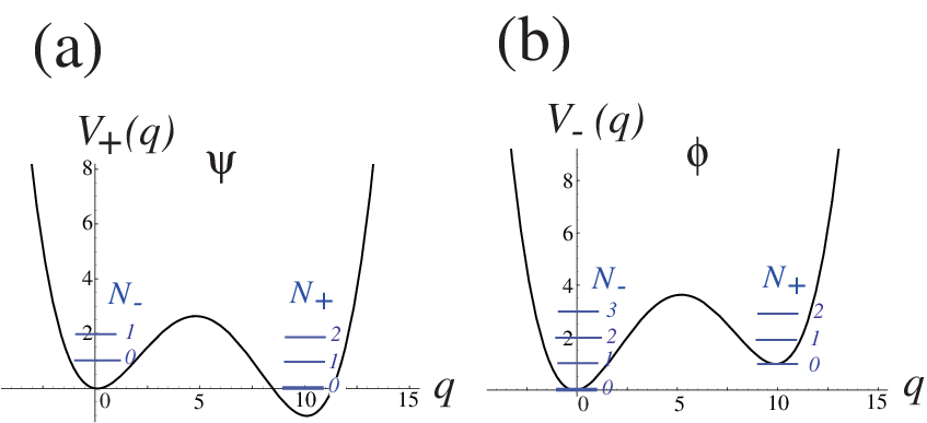
Figure 7: (Color online) The asymmetric double-well potential (a) given by (102) with g=0.1g=0.1, and (b) given by (103) with g=0.1g=0.1. Energy levels around q=0q=0 and q=1/gq=1/g are also shown.

Identifying 𝒬{\cal Q} with a generator of supersymmetry, we have the supersymmetric Hamiltonian ℋ=𝒬2{\cal H}={\cal Q}^{2}, which satisfies

ℋ⁡(ψ⁡(x)ϕ⁡(x))=E2​(ψ⁡(x)ϕ⁡(x)).\displaystyle{\cal H}\left(\begin{array}[]{c}{\psi(x)}\\ {\phi(x)}\end{array}\right)=E^{2}\left(\begin{array}[]{c}{\psi(x)}\\ {\phi(x)}\end{array}\right).

By using the following variable qq,

x+Gπ​Φ=q​1π​G​Φ,\displaystyle x+\frac{G}{\pi\Phi}=q\sqrt{\frac{1}{\pi G\Phi}}, (95)

(IV.2) can be rewritten as

[−12​d2d​q2+12​q2​(1−g​q)2−(g​q−12)​σz]​(ψ⁡(q)ϕ⁡(q))=ℰ​(ψ⁡(q)ϕ⁡(q)),\displaystyle\left[-\frac{1}{2}\frac{d^{2}}{dq^{2}}+\frac{1}{2}q^{2}(1-gq)^{2}-\left(gq-\frac{1}{2}\right)\sigma_{z}\right]\left(\begin{array}[]{c}{\psi(q)}\\ {\phi(q)}\end{array}\right)={\cal E}\left(\begin{array}[]{c}{\psi(q)}\\ {\phi(q)}\end{array}\right),

with

g=12​G​π​ΦG,ℰ=18​π​Φ​G​E2.\displaystyle g=\frac{1}{2G}\sqrt{\frac{\pi\Phi}{G}},\quad{\cal E}=\frac{1}{8\pi\Phi G}E^{2}. (101)

Therefore, the potential terms for ψ⁡(x){\psi(x)} and ϕ⁡(x){\phi(x)} are given by

V+​(q)=12​q2​(1−g​q)2−g​q,\displaystyle V_{+}(q)=\frac{1}{2}q^{2}(1-gq)^{2}-gq, (102)

and

V−​(q)=12​q2​(1−g​q)2+g​q,\displaystyle V_{-}(q)=\frac{1}{2}q^{2}(1-gq)^{2}+gq, (103)

respectively (see Fig.7).

In the leading order of gg, the potentials (102) and (103) are well approximated by the harmonic oscillator around q=0q=0 and q=1/gq=1/g. Around q=0q=0, (IV.2) becomes

[−12​d2d​q2+12​q2+12​σz]​(ψ⁡(q)ϕ⁡(q))=ℰ​(ψ⁡(q)ϕ⁡(q)),\displaystyle\left[-\frac{1}{2}\frac{d^{2}}{dq^{2}}+\frac{1}{2}q^{2}+\frac{1}{2}\sigma_{z}\right]\left(\begin{array}[]{c}{\psi(q)}\\ {\phi(q)}\end{array}\right)={\cal E}\left(\begin{array}[]{c}{\psi(q)}\\ {\phi(q)}\end{array}\right),

and around q=1/gq=1/g, (IV.2) becomes

[−12​d2d​q2+12​(q−1g)2−12​σz]​(ψ⁡(q)ϕ⁡(q))=ℰ​(ψ⁡(q)ϕ⁡(q)).\displaystyle\left[-\frac{1}{2}\frac{d^{2}}{dq^{2}}+\frac{1}{2}\left(q-\frac{1}{g}\right)^{2}-\frac{1}{2}\sigma_{z}\right]\left(\begin{array}[]{c}{\psi(q)}\\ {\phi(q)}\end{array}\right)={\cal E}\left(\begin{array}[]{c}{\psi(q)}\\ {\phi(q)}\end{array}\right).

Therefore, the energy levels for ψ{\psi} around q=1/gq=1/g and q=0q=0 are given by

ℰN+=N+,(N+=0,1,2,…),\displaystyle{\cal E}_{N_{+}}=N_{+},\quad(N_{+}=0,1,2,\ldots), (114)

and

ℰN−=N−+1,(N−=0,1,2,…),\displaystyle{\cal E}_{N_{-}}=N_{-}+1,\quad(N_{-}=0,1,2,\ldots), (115)

respectively, and those for ϕ{\phi} around q=1/gq=1/g and q=0q=0 are given by

ℰN+=N++1,(N+=0,1,2,…),\displaystyle{\cal E}_{N_{+}}=N_{+}+1,\quad(N_{+}=0,1,2,\ldots), (116)

and

ℰN−=N−,(N−=0,1,2,…),\displaystyle{\cal E}_{N_{-}}=N_{-},\quad(N_{-}=0,1,2,\ldots), (117)

respectively.

Now take into account tunneling effects between the energy levels around q=0q=0 and q=1/gq=1/g. The tunneling effects can be estimated by the WKB method presented in Appendix D of Ref.[32]. Here we consider only the equation for ψ⁡(q){\psi(q)} since the equation for ϕ⁡(q){\phi(q)} gives the same result. The solution of (IV.2) which vanishes for q→−∞q\to-\infty is given by

ψ⁡(q)=A​Dν​(−2​q),\displaystyle{\psi}(q)=AD_{\nu}\left(-\sqrt{2}q\right), (118)

where ν=ℰ−1\nu={\cal E}-1, AA is a constant, and DνD_{\nu} the parabolic cylinder function[33]. The solution of (IV.2) which vanishes for q→∞q\to\infty is

ψ⁡(q)=A~​Dν+1​[2​(q−1/g)],\displaystyle{\psi}(q)=\tilde{A}D_{\nu+1}\left[\sqrt{2}\left(q-1/g\right)\right], (119)

where A~\tilde{A} is a constant. We connect these solutions (118) and (119) with that in the forbidden region. In the forbidden region, the usual semi-classical expression for the wave function is available:

ψ(q)=C1k⁡(q)exp(−∫q1qk(x)dx)+C2k⁡(q)exp(∫q1qk(x)dx),\displaystyle{\psi}(q)=\frac{C_{1}}{\sqrt{k(q)}}\exp\left(-\int_{q_{1}}^{q}k(x)dx\right)+\frac{C_{2}}{\sqrt{k(q)}}\exp\left(\int_{q_{1}}^{q}k(x)dx\right), (120)

where k⁡(q)=2​(V+​(q)−ℰ)k(q)=\sqrt{2(V_{+}(q)-{\cal E})} with V+​(q)V_{+}(q) in (102), qiq_{i} (i=1,2)(i=1,2) are the turning points, V+​(qi)=ℰV_{+}(q_{i})={\cal E}, and CiC_{i} (i=1,2)(i=1,2) are constants. Connecting (118) with (120), and (119) with (120), we obtain

γ2​(−2g2)2​ℰ−1​Γ​(1−ℰ)​Γ​(−ℰ)=1,γ=e−1/6g2g​π1/2.\displaystyle\gamma^{2}\left(-\frac{2}{g^{2}}\right)^{2{\cal E}-1}\Gamma\left(1-{\cal E}\right)\Gamma\left(-{\cal E}\right)=1,\quad\gamma=\frac{e^{-1/6g^{2}}}{g\pi^{1/2}}. (121)

For ℰ{\cal E} near zero energy (ℰ≪1{\cal E}\ll 1), we have

(−2g2)2​ℰ−1≃−g22,Γ⁡(1−ℰ)≃1,Γ⁡(−ℰ)≃−1ℰ,\displaystyle\left(-\frac{2}{g^{2}}\right)^{2{\cal E}-1}\simeq-\frac{g^{2}}{2},\quad\Gamma\left(1-{\cal E}\right)\simeq 1,\quad\Gamma\left(-{\cal E}\right)\simeq-\frac{1}{{\cal E}}, (122)

thus the solution of (121) for g≪1g\ll 1 is obtained as

ℰ(=18​π​Φ​G​E2)=γ2​g22.\displaystyle{\cal E}\left(=\frac{1}{8\pi\Phi G}{E}^{2}\right)=\gamma^{2}\frac{g^{2}}{2}. (123)

This implies that the gap around E=0E=0 is given by

Δ​E=4​Φ​G​exp⁡(−2​G33​π​Φ),\displaystyle\Delta E=4\sqrt{\Phi G}\exp\left(-\frac{2G^{3}}{3\pi\Phi}\right), (124)

and the exponent α\alpha in (70) is given by

α=23​π​G3=23​π​(2−t)3/2≡αWKB,(0<2−t≪1).\displaystyle\alpha=\frac{2}{3\pi}G^{3}=\frac{2}{3\pi}(2-t)^{3/2}\equiv\alpha_{\rm WKB},\quad(0<2-t\ll 1). (125)
Refer to caption
Figure 8: (Color online) α\alpha as a function of tt, where those obtained from numerical calculations and the WKB analysis are shown by points and the line, respectively.
Table 1: α\alpha for several tt obtained from numerical calculations and the WKB analysis. The relative discrepancies between them, δ\delta, are also shown.
tt α\alpha αWKB\alpha_{\rm WKB} δ\delta
1.6 6.523×10−26.523\times 10^{-2} 5.368×10−25.368\times 10^{-2} 0.177
1.65 5.198×10−25.198\times 10^{-2} 4.394×10−24.394\times 10^{-2} 0.155
1.7 4.076×10−24.076\times 10^{-2} 3.487×10−23.487\times 10^{-2} 0.145
1.75 3.042×10−23.042\times 10^{-2} 2.653×10−22.653\times 10^{-2} 0.128
1.8 2.140×10−22.140\times 10^{-2} 1.898×10−21.898\times 10^{-2} 0.113
1.85 1.369×10−21.369\times 10^{-2} 1.233×10−21.233\times 10^{-2} 0.0993
1.9 7.294×10−37.294\times 10^{-3} 6.711×10−36.711\times 10^{-3} 0.0799
1.95 2.555×10−32.555\times 10^{-3} 2.373×10−32.373\times 10^{-3} 0.0712

Now we compare (125) with those obtained numerically for a small Φ\Phi. In Fig.8, we show α\alpha as a function of tt, and in Table 1, we list them. The relative discrepancy

δ≡|αWKB−αα|,\displaystyle\delta\equiv\left|\frac{\alpha_{\rm WKB}-\alpha}{\alpha}\right|, (126)

decreases as tt approaches 22. This is because the neglected terms O⁡(py4)O(p_{y}^{4}) in (73) come to be smaller and smaller as tt approaches 22.

IV.3 t=2t=2

Refer to caption
Figure 9: (Color online) (a)Energy bands as a function of Φ\Phi for t=2.0t=2.0. (b)The three lowest bands in E≥0E\geq 0 in the log-log scale.

At t=2t=2, the two Dirac zero modes at Φ=0\Phi=0 merge into the confluent point (17). As a consequence, a gap around E=0E=0 in a weak magnetic field makes a transition from an exponential (non-perturbative) to a power-law (perturbative) behavior as a function of Φ\Phi.

In Fig.9(a), we show the energy bands as a function of Φ\Phi for t=2.0t=2.0. We show the three lowest bands in E≥0E\geq 0 in the log-log scale for weak magnetic field in Fig.9(b). We fit our data by

E∼Φκ.\displaystyle E\sim\Phi^{\kappa}. (127)

For t=2.0t=2.0, we obtain the exponent κ\kappa as κ∼0.66\kappa\sim 0.66, 0.650.65, and 0.650.65 for the lowest, the second lowest, and the third lowest bands in E≥0E\geq 0, respectively. Thus for t=2.0t=2.0 we have a power-law behavior E∼±Φ2/3E\sim\pm\Phi^{2/3}.

The behavior E∼±Φ2/3E\sim\pm\Phi^{2/3} is derived analytically from a particular dispersion relation at t=2t=2 for Φ=0\Phi=0 [25]. For Φ=0\Phi=0, (12) and (73) with G=0G=0 give

E=±4​px2+py4,\displaystyle E=\pm\sqrt{4p_{x}^{2}+p_{y}^{4}}, (128)

which is linear in one direction and quadratic in the other. The exponent κ\kappa is obtained from S⁡(E)∼ΦS(E)\sim\Phi, where S⁡(E)S(E) is the area surrounded by an orbit of energy EE in the momentum space [25]. From (128), we have

S⁡(E)=Γ​(1/4)23​2​π​|E|3/2,\displaystyle S(E)=\frac{\Gamma(1/4)^{2}}{3\sqrt{2\pi}}|E|^{3/2}, (129)

thus E∼±Φ2/3E\sim\pm\Phi^{2/3}.

IV.4 t>2t>2

Refer to caption
Figure 10: (Color online) Energy bands as a function of Φ\Phi for t=2.5t=2.5 and t=3.0t=3.0.
Refer to caption
Figure 11: (Color online) A closer look of Fig.10 in a weak magnetic field region. The expressions (133) for n=0,1,2n=0,1,2 are also shown by the red lines.

For t>2t>2, we do not have zero modes but have a gap around E=0E=0. In Fig.10, we show two examples of the energy bands as a function of Φ\Phi for t>2t>2.

Let us study behavior of energy bands in a weak magnetic field by the continuum approximation. For Φ=0\Phi=0, we expand kxk_{x} and kyk_{y} around (kx,ky)=(π,0)(k_{x},k_{y})=(\pi,0),

kx=π+px,ky=py,(|px|,|py|≪1),\displaystyle k_{x}=\pi+p_{x},\quad k_{y}=p_{y},\quad(|p_{x}|,|p_{y}|\ll 1), (130)

then (12) gives

E=±Eg2+2​t​px2+2​(t−2)​py2,Eg=t−2.\displaystyle E=\pm\sqrt{E_{g}^{2}+2tp_{x}^{2}+2(t-2)p_{y}^{2}},\quad E_{g}=t-2. (131)

Thus for small |px||p_{x}| and |py||p_{y}| (|px|,|py|≪Eg|p_{x}|,|p_{y}|\ll E_{g}), (131) is written as

E=±(Eg+tt−2​px2+py2),\displaystyle E=\pm\left(E_{g}+\frac{t}{t-2}p_{x}^{2}+p_{y}^{2}\right), (132)

which is quadratic in both pxp_{x} and pyp_{y}. In the continuum approximation, we put px→p^xp_{x}\to\hat{p}_{x} and py→p^y+B​xp_{y}\to\hat{p}_{y}+Bx with p^x=−i∂x\hat{p}_{x}=-i\partial_{x}, p^y=−i∂y\hat{p}_{y}=-i\partial_{y} and B=π​ΦB=\pi\Phi. Then we have

E=±Eg​[1+2​π​t​(n+12)​Φ(t−2)3/2],(n=0,1,2,…),\displaystyle E=\pm E_{g}\left[1+2\pi\sqrt{t}\left(n+\frac{1}{2}\right)\frac{\Phi}{(t-2)^{3/2}}\right],\quad(n=0,1,2,\ldots), (133)

where we have neglected higher order corrections of O⁡((2​π​t​(n+1/2)​Φ(t−2)3/2)2)O\left(\left(\frac{2\pi\sqrt{t}(n+1/2)\Phi}{(t-2)^{3/2}}\right)^{2}\right). The energy bands in the weak magnetic field limit (Φ≪(t−2)3/22​π​t​(n+1/2))\left(\Phi\ll\frac{(t-2)^{3/2}}{2\pi\sqrt{t}(n+1/2)}\right) are well approximated by (133), which is seen in Fig.11. We note that, for t∼2t\sim 2, the neglected higher order corrections of O⁡((2​π​t​(n+1/2)​Φ(t−2)3/2)2)O\left(\left(\frac{2\pi\sqrt{t}(n+1/2)\Phi}{(t-2)^{3/2}}\right)^{2}\right) can not be neglected. However, they become small for t≫2t\gg 2, and the energy bands in a weak magnetic field are well fitted by (133). This result is consistent with the fact that the honeycomb lattice becomes equivalent to the square lattice for t≫2t\gg 2[26, 9].

We summarize our results of this section in Fig.12.

Refer to caption
Figure 12: (Color online) (a)Behavior of a gap Δ​E\Delta E around E=0E=0 as a function of tt in a weak magnetic field. (The nearest bands to E=0E=0 show the same behavior as Δ​E\Delta E.) (b)Behavior of the other energy bands for E≈0E\approx 0 as a function of tt in a weak magnetic field.

V E=0E=0 edge states in anisotropic honeycomb lattice

Refer to caption
Figure 13: (Color online) Honeycomb lattices with zigzag and bearded edges (Lx=7L_{x}=7). The left and the right edges are the zigzag and the bearded edges, respectively.

In this section, we examine E=0E=0 edge states. The condition for the existence of zero energy edge states in a magnetic field is analytically derived. On the basis of it, it turns out that the anisotropy of the hopping integrals induces abrupt changes of the number of zero energy edge states, which depend on the shapes of the edges sensitively.

In order to see this, we focus on the honeycomb lattices with zigzag and bearded edges as shown in Fig.13. For these lattices, we have edges along the yy-direction. Let us impose the periodic boundary condition along the yy-direction:

ψn,m+2​Ly=ψn,m,ϕn,m+2​Ly=ϕn,m,\displaystyle\psi_{n,m+2L_{y}}=\psi_{n,m},\quad\phi_{n,m+2L_{y}}=\phi_{n,m}, (134)

where an integer LyL_{y} denotes the circumference of the cylinder. Then one can write

ψn,m=exp⁡(i​ky2​m)​ψn,ϕn,m=exp⁡(i​ky2​m)​ϕn.\displaystyle\psi_{n,m}=\exp\left(i\frac{k_{y}}{2}m\right)\psi_{n},\quad\phi_{n,m}=\exp\left(i\frac{k_{y}}{2}m\right)\phi_{n}. (135)

Let us focus on E=0E=0 states. In the same manner as Sec.III.2, for E=0E=0 and Φ=p/q\Phi=p/q with coprime integers pp and qq, the amplitudes of wavefunctions separated by a distance qq are found to satisfy

|ψ(N+1)​q+l|=r​|ψN​q+l|,|ϕN​q+l|=r​|ϕ(N+1)​q+l|,\displaystyle|\psi_{(N+1)q+l}|=r|\psi_{Nq+l}|,\quad|\phi_{Nq+l}|=r|\phi_{(N+1)q+l}|,
(l=0,1,2,…,q−1),\displaystyle(l=0,1,2,\ldots,q-1), (136)

with

r≡2tq​|cos⁡(q​ky2+q+12​π)|.\displaystyle r\equiv\frac{2}{t^{q}}\left|\cos\left(q\frac{k_{y}}{2}+\frac{q+1}{2}\pi\right)\right|. (137)

From (136), we have

|ψN​q+l|=rN​|ψl|,|ϕl|=rN​|ϕN​q+l|.\displaystyle|\psi_{Nq+l}|=r^{N}|\psi_{l}|,\quad|\phi_{l}|=r^{N}|\phi_{Nq+l}|. (138)

The boundary conditions for the zigzag and the bearded edges are given by

ϕ0=0,ϕL​x+1=0,\displaystyle\phi_{0}=0,\quad\phi_{Lx+1}=0, (139)

respectively. These boundary conditions give ϕn=0\phi_{n}=0 for all nn, thus we consider only ψn\psi_{n} in the following.

Suppose that LxL_{x} is large enough: Lx≫qL_{x}\gg q. Then from (138), if r<1r<1 (r>1r>1) we have E=0E=0 states on the zigzag edge (bearded edge). For t>21/qt>2^{1/q}, r<1r<1 is satisfied for all values of kyk_{y}, but r>1r>1 is not satisfied for any values of kyk_{y}. Thus we have E=0E=0 states localized on the zigzag edge for all values of kyk_{y}, but we do not have E=0E=0 states localized on the bearded edge for any values of kyk_{y}. For t<21/qt<2^{1/q}, E=0E=0 edge states exist both on the zigzag and the bearded edge. The total width dzigzag​(t,q)d_{\rm zigzag}(t,q) of the region of kyk_{y} which gives E=0E=0 states on the zigzag edge is given by

dzigzag​(t,q)=2​(π−2​cos−1⁡tq2),\displaystyle d_{\rm zigzag}(t,q)=2\left(\pi-2\cos^{-1}\frac{t^{q}}{2}\right), (140)

and that for the bearded edge, dbearded​(t,q)d_{\rm bearded}(t,q), is given by

dbearded​(t,q)=2​π−dzigzag​(t,q)=4​cos−1⁡tq2.\displaystyle d_{\rm bearded}(t,q)=2\pi-d_{\rm zigzag}(t,q)=4\cos^{-1}\frac{t^{q}}{2}. (141)

For a fixed value of Φ\Phi, dzigzagd_{\rm zigzag} (dbeardedd_{\rm bearded}) increases (decreases) as tt increases in the region of 0<t<21/q0<t<2^{1/q}. At t=21/qt=2^{1/q}, dzigzagd_{\rm zigzag} covers the whole region of kyk_{y}, and dbeardedd_{\rm bearded} vanishes. For t>21/qt>2^{1/q}, we have E=0E=0 edge states on the zigzag edges for all values of kyk_{y}. We show examples of the energy spectra of honeycomb lattices with zigzag and bearded edges in Figs.14 and 15.

Effects of the anisotropy of the hopping integrals are evident in a weak magnetic field, Φ≪1\Phi\ll 1 (q≫1q\gg 1). For t=1t=1, dzigzagd_{\rm zigzag} and dbeardedd_{\rm bearded} do not depend on the magnetic field, and are given by dzigzag=2​π3d_{\rm zigzag}=\frac{2\pi}{3} and dbearded=4​π3d_{\rm bearded}=\frac{4\pi}{3}, respectively. However, for t<1t<1, dzigzagd_{\rm zigzag} decreases toward 00 and dbeardedd_{\rm bearded} increases toward 2​π2\pi as qq increases. In contrast, for t>1t>1, dzigzagd_{\rm zigzag} (dbeardedd_{\rm bearded}) increases (decreases) as qq increases and reaches 2​π2\pi (00) at q=ln⁡2/ln⁡tq=\ln 2/\ln t. Note that even in a small anisotropy, dzigzagd_{\rm zigzag} and dbeardedd_{\rm bearded} change abruptly in a weak magnetic field (q≫1q\gg 1).

Instead of dzigzagd_{\rm zigzag} and dbeardedd_{\rm bearded}, we also consider the integrated charge density InI_{n} for E=0E=0 edge states[21, 22]:

In=∫|ψn​(ky)|2​d​ky,\displaystyle I_{n}=\int{|\psi_{n}(k_{y})|^{2}dk_{y}}, (142)

where the normalization condition is imposed on ψn​(ky)\psi_{n}(k_{y}),

∑n=0Lx|ψn​(ky)|2=1.\displaystyle\sum_{n=0}^{L_{x}}|\psi_{n}(k_{y})|^{2}=1. (143)

To characterize the numbers of the states localized on the edges, we introduce the following quantities,

Nzigzag=∑n=0q−1In,Nbearded=∑n=Lx−q+1LxIn.\displaystyle N_{\rm zigzag}=\sum_{n=0}^{q-1}I_{n},\quad N_{\rm bearded}=\sum_{n=L_{x}-q+1}^{L_{x}}I_{n}. (144)

For r<1r<1, only the zigzag edge has E=0E=0 modes, and NzigzagN_{\rm zigzag} is evaluated as

Nzigzag=∫(1−2t2​q)​d​ky+(−1)q​2t2​q​∫cos⁡(q​ky)​d​ky,\displaystyle N_{\rm zigzag}=\int\left(1-\frac{2}{t^{2q}}\right)dk_{y}+(-1)^{q}\frac{2}{t^{2q}}\int\cos(qk_{y})dk_{y}, (145)

where the domain of the integration is restricted to those kyk_{y} with r<1r<1. Here we have used the relation derived from (138) and (143):

∑j=0⌊(Lx+1)/q⌋−1r2​j​∑n=0q−1|ψn​(ky)|2+O⁡(r2​Lx/q)=1,\displaystyle\sum_{j=0}^{\lfloor{(L_{x}+1)/q}\rfloor-1}r^{2j}\sum_{n=0}^{q-1}|\psi_{n}(k_{y})|^{2}+O(r^{2L_{x}/q})=1, (146)

where O⁡(r2​Lx/q)O(r^{2L_{x}/q}) corrections can be neglected since r<1r<1 and Lx≫qL_{x}\gg q. (⌊x⌋\lfloor{x}\rfloor denotes the integer part of xx.) Eq. (146) is rewritten as

∑n=0q−1|ψn​(ky)|2=1−r2+O⁡(r2​Lx/q),\displaystyle\sum_{n=0}^{q-1}|\psi_{n}(k_{y})|^{2}=1-r^{2}+O(r^{2L_{x}/q}), (147)

then substituting this into the first equation in (144) and using (137), we obtain Eq. (145). On the other hand, for r>1r>1, we have E=0E=0 modes only on the bearded edge, and NbeardedN_{\rm bearded} is given by

Nbearded=∫d​ky−t2​q4​∫1cos2⁡(q​ky2+q+12​π)​d​ky,\displaystyle N_{\rm bearded}=\int dk_{y}-\frac{t^{2q}}{4}\int\frac{1}{\cos^{2}\left(q\frac{k_{y}}{2}+\frac{q+1}{2}\pi\right)}dk_{y}, (148)

where the domain of the integration is restricted to those kyk_{y} with r>1r>1. Here we have used the relation

∑n=Lx−q+1Lx|ψn(ky)|2=1−r−2+O(r−2Lx/q),\displaystyle\sum_{n=L_{x}-q+1}^{L_{x}}|\psi_{n}(k_{y})|^{2}=1-r^{-2}+O(r^{-2L_{x}/q}), (149)

which is derived from (138) and (143) in a similar manner as Eq. (147).

Let us now evaluate NzigzagN_{\rm zigzag} and NbeardedN_{\rm bearded} from (145) and (148). For t>21/qt>2^{1/q}, r<1r<1 is realized for all values of kyk_{y} as shown above. Therefore,

Nzigzag\displaystyle N_{\rm zigzag} =\displaystyle= ∫02​π(1−2t2​q)​d​ky+(−1)q​2t2​q​∫02​πcos⁡(q​ky)​d​ky\displaystyle\int_{0}^{2\pi}\left(1-\frac{2}{t^{2q}}\right)dk_{y}+(-1)^{q}\frac{2}{t^{2q}}\int_{0}^{2\pi}\cos(qk_{y})dk_{y}
=\displaystyle= 2​π​(1−2t2​q),\displaystyle 2\pi\left(1-\frac{2}{t^{2q}}\right),
Nbearded\displaystyle N_{\rm bearded} =\displaystyle= 0.\displaystyle 0. (150)

For t<21/qt<2^{1/q}, either r>1r>1 or r<1r<1 is realized by a suitable choice of kyk_{y}. Thus both NzigzagN_{\rm zigzag} and NbeardedN_{\rm bearded} become nonzero as,

Nzigzag\displaystyle N_{\rm zigzag} =\displaystyle= dzigzag(1−2t2​q)−4t2​q∫2​cos−1⁡tq2πcoskydky\displaystyle d_{{\rm zigzag}}\left(1-\frac{2}{t^{2q}}\right)-\frac{4}{t^{2q}}\int_{2\cos^{-1}\frac{t^{q}}{2}}^{\pi}\cos k_{y}dk_{y}
=\displaystyle= 2​(π−2​cos−1⁡tq2)​(1−2t2​q)+4tq​sin⁡(cos−1⁡tq2),\displaystyle 2\left(\pi-2\cos^{-1}\frac{t^{q}}{2}\right)\left(1-\frac{2}{t^{2q}}\right)+\frac{4}{t^{q}}\sin\left(\cos^{-1}\frac{t^{q}}{2}\right),
Nbearded\displaystyle N_{\rm bearded} =\displaystyle= dbearded−t2​q2​∫02​cos−1⁡tq21cos2⁡(ky2)​d​ky\displaystyle d_{{\rm bearded}}-\frac{t^{2q}}{2}\int_{0}^{2\cos^{-1}\frac{t^{q}}{2}}\frac{1}{\cos^{2}\left(\frac{k_{y}}{2}\right)}dk_{y} (151)
=\displaystyle= 4​cos−1⁡tq2−2​tq​sin⁡(cos−1⁡tq2).\displaystyle 4\cos^{-1}\frac{t^{q}}{2}-2t^{q}\sin\left(\cos^{-1}\frac{t^{q}}{2}\right).

We also find that for t=1t=1, NzigzagN_{\rm zigzag} and NbeardedN_{\rm bearded} are independent of Φ\Phi,

Nzigzag=2​3−2​π3,Nbearded=43​π−3.\displaystyle N_{\rm zigzag}=2\sqrt{3}-\frac{2\pi}{3},\quad N_{\rm bearded}=\frac{4}{3}\pi-\sqrt{3}. (152)

These formulas also show that a small anisotropy induces sudden changes of the edge states in a weak magnetic field: When qq increases for a fixed t>1t>1, NzigzagN_{\rm zigzag} increases toward 2​π2\pi and NbeardedN_{\rm bearded} reaches zero at q=ln⁡2/ln⁡tq=\ln 2/\ln t. And for a fixed t<1t<1, NzigzagN_{\rm zigzag} goes to zero and NbeardedN_{\rm bearded} increases toward 2​π2\pi as qq increases. Thus in a weak magnetic field (q≫1q\gg 1), there are abrupt changes in NzigzagN_{\rm zigzag} and NbeardedN_{\rm bearded} at t=1t=1.

In Figs.16 and 17, we show scaled plots of InI_{n} as a function of n/qn/q. Here we have taken Lx=6​qL_{x}=6q. Because of the normalization condition (143), InI_{n} decreases as ∼1/Lx\sim 1/L_{x} when LxL_{x} increases. To remove the artificial dependence on LxL_{x}, we plot q​InqI_{n} instead of InI_{n}. For t=1t=1, q​InqI_{n}’s for different Φ(=p/q)\Phi(=p/q)’s with the same pp fall on a common curve[22]. However, for t>1t>1, q​InqI_{n} comes to be localized on qq sites from the zigzag edges as Φ\Phi (with the same pp) decreases. In contrast, for t<1t<1, q​InqI_{n} comes to be localized on qq sites from the bearded edges as Φ\Phi (with the same pp) decreases. In Table 2, we also compare numerical data and analytical results presented above. With relative discrepancies less than 10%10\%, they exhibit good agreements.

So far, we have assumed that Lx≫qL_{x}\gg q. When Lx≲qL_{x}\lesssim q, the above arguments cannot be justified. However, numerical calculations suggest that if Lx≫1/ΦL_{x}\gg 1/\Phi (p​Lx≫qpL_{x}\gg q), the particular edge states presented above appear again. In Fig.18, we show the energy bands for Lx=50L_{x}=50 and Φ=1001/5000(∼1/5)\Phi=1001/5000(\sim 1/5), which are found to be indistinguishable from those for Φ=1/5\Phi=1/5 (Fig.14). It is also found that if the magnetic field decreases and Lx≲1/ΦL_{x}\lesssim 1/\Phi is realized, then the energy bands approach those without a magnetic field, which is illustrated in Fig.19.

Refer to caption
Figure 14: (Color online) Energy spectra of honeycomb lattices with zigzag and bearded edges for Φ=1/5\Phi=1/5 and Lx=50L_{x}=50. (a) t=0.9t=0.9, (b) t=1.0t=1.0, (c) t=21/5(∼1.15)t=2^{1/5}(\sim 1.15) (d) t=1.5t=1.5. The E=0E=0 edge states localized on the zigzag edges are on the blue lines, and those localized on the bearded edges are on the red lines.
Refer to caption
Figure 15: (Color online) A closer look of Fig.14 at E≈0E\approx 0.
Refer to caption
Figure 16: (Color online) q​InqI_{n} as a function of n/qn/q for Φ=1/11\Phi=1/11, 1/171/17, and 1/211/21. (a) t=1.0t=1.0, (b) t=1.07t=1.07, (c) t=0.97t=0.97.
Refer to caption
Figure 17: (Color online) q​InqI_{n} as a function of n/qn/q for Φ=2/11\Phi=2/11, 2/172/17, and 2/212/21. (a) t=1.0t=1.0, (b) t=1.07t=1.07, (c) t=0.97t=0.97.
Table 2: Numerical data, NzigzagN_{\rm zigzag}, NbeardedN_{\rm bearded}, and analytical results, Nzigzag(A)N_{\rm zigzag}^{(\rm A)}, Nbearded(A)N_{\rm bearded}^{(\rm A)}. (a) t=1.0t=1.0 (b) t=1.07t=1.07 (c) t=0.97t=0.97. The relative discrepancies between numerical data and analytical results, δzigzag=|(Nzigzag(A)−Nzigzag)/Nzigzag|\delta_{\rm zigzag}=|(N_{\rm zigzag}^{(\rm A)}-N_{\rm zigzag})/N_{\rm zigzag}| and δbearded=|(Nbearded(A)−Nbearded)/Nbearded|\delta_{\rm bearded}=|(N_{\rm bearded}^{(\rm A)}-N_{\rm bearded})/N_{\rm bearded}|, are also shown.
(a) t=1.0t=1.0
Φ\Phi NzigzagN_{\rm zigzag} NbeardedN_{\rm bearded} Nzigzag(A)N_{\rm zigzag}^{(\rm A)} Nbearded(A)N_{\rm bearded}^{(\rm A)} δzigzag\delta_{\rm zigzag} δbearded\delta_{\rm bearded}
1/11 1.484 2.562 0.0770 0.0411
2/11 1.484 2.562 0.0770 0.0411
1/17 1.485 2.563 2​3−23​π2\sqrt{3}-\frac{2}{3}\pi 43​π−3\frac{4}{3}\pi-\sqrt{3} 0.0776 0.0415
2/17 1.485 2.563 0.0776 0.0415
1/21 1.486 2.563 0.0783 0.0415
2/21 1.486 2.563 0.0783 0.0415
(b) t=1.07t=1.07
Φ\Phi NzigzagN_{\rm zigzag} NbeardedN_{\rm bearded} Nzigzag(A)N_{\rm zigzag}^{(\rm A)} Nbearded(A)N_{\rm bearded}^{(\rm A)} δzigzag\delta_{\rm zigzag} δbearded\delta_{\rm bearded}
1/11 3.635 0.2336 3.447 0.0517
2/11 3.635 0.2335 0.0517
1/17 5.027 0.009609 5.024 0 0.000597 -
2/17 5.027 0.009591 0.000597
1/21 5.550 0.0007872 5.550 0.00
2/21 5.550 0.0007847 0.00
(c) t=0.97t=0.97
Φ\Phi NzigzagN_{\rm zigzag} NbeardedN_{\rm bearded} Nzigzag(A)N_{\rm zigzag}^{(\rm A)} Nbearded(A)N_{\rm bearded}^{(\rm A)} δzigzag\delta_{\rm zigzag} δbearded\delta_{\rm bearded}
1/11 1.040 3.553 0.9665 3.484 0.0707 0.0194
2/11 1.040 3.553 0.0707 0.0194
1/17 0.8618 3.992 0.8017 3.936 0.0697 0.0140
2/17 0.8618 3.992 0.0697 0.0140
1/21 0.7610 4.248 0.7083 4.198 0.0693 0.0118
2/21 0.7610 4.248 0.0693 0.0118
Refer to caption
Figure 18: Energy spectra of honeycomb lattices with zigzag and bearded edges for Φ=1001/5000(∼1/5)\Phi=1001/5000(\sim 1/5) and Lx=50L_{x}=50. (a) t=0.9t=0.9, (b) t=1.0t=1.0, (c) t=21/5(∼1.15)t=2^{1/5}(\sim 1.15) (d) t=1.5t=1.5.
Refer to caption
Figure 19: Energy spectra of honeycomb lattices with zigzag and bearded edges for t=1.5t=1.5 and Lx=50L_{x}=50. (a) Φ=1001/5000\Phi=1001/5000, (b) Φ=101/5000\Phi=101/5000, (c) Φ=11/5000\Phi=11/5000, (d) Φ=1/5000\Phi=1/5000. We also show energy bands in the absence of a magnetic field in (e).

VI Summary and discussion

In this paper, we examined behavior of zero modes and a gap around zero energy for a tight-binding model on the anisotropic honeycomb lattice in a magnetic field, whose anisotropy is controlled by the hopping parameter tt. It was found that zero modes exist for all (rational) Φ\Phi for 0<t≤10<t\leq 1, and a gap around zero energy opens by a tiny anisotropy for the graphene in a magnetic field. This is contrasted with the case for the square lattice, where zero modes always exist for all (rational) Φ\Phi when we change the ratio of the hopping parameters tx/tyt_{x}/t_{y}[34]. For 1<t<21<t<2, a gap around zero energy in a weak magnetic field behaves as a non-perturbative and exponential form as a function of the magnetic field. This non-analytic behavior is naturally explained by tunneling effects between energy levels around two Dirac zero modes in the absence of a magnetic field. At t=2t=2, the gap around zero energy in a weak magnetic field makes a transition from an exponential (non-perturbative) to a power-law (perturbative) behavior as a function of the magnetic field. In particular, an explicit form of the gap around zero energy near the transition point is obtained by the WKB method. For t>2t>2, energy bands in a weak magnetic field show linear dependence on a magnetic field.

We also examined edge states with zero energy. The condition for the existence of zero energy edge states in a magnetic field is analytically derived. On the basis of the condition, it is found that the anisotropy of the hopping integrals induces abrupt changes of the number of zero energy edge states, which depend on the shapes of the edges sensitively.

Finally, we would like to discuss possible experimental realization of anisotropy of the hopping integrals. Recently, it was experimentally found that a reversible and controlled uniaxial strain can be produced in graphene[36, 35]. Therefore, we can expect that a small anisotropy of the hopping integrals is realized by the uniaxial strain. On the other hand, in order to realize a large anisotropy such as t∼2t\sim 2, cold atoms in optical honeycomb lattices created by laser beams would serve as alternatives[25]. In these lattices, a large anisotropy could be induced and controlled by changing the intensities of the laser fields[37]. In addition, by using Raman processes induced by laser fields, effective magnetic fields can be generated in the optical lattice[38].

Note added. After submission of this paper, we became aware of recent independent work which has some overlap with ours for t∼2t\sim 2[39, 40]. We are grateful to G. Montambaux for pointing out these papers.

Acknowledgements.
This work was supported in part by Global COE Program “the Physical Sciences Frontier,” MEXT, Japan for K. E. This work was also supported in part by NSF grant DMR-05-41988 for B. I. Halperin.

Appendix A Tight-binding model on a honeycomb lattice with a variable lattice spacing

Refer to caption
Figure 20: A honeycomb lattice with a variable lattice spacing. If a=3​ba=\sqrt{3}b, we have the hexagonal symmetry for each sublattice.

In this appendix, we consider a honeycomb lattice with a variable lattice spacing shown in Fig.20. The tight-binding equation in a magnetic field is given by

E​ψ​(x,y)\displaystyle E\psi(x,y) =\displaystyle= ty​[ϕ⁡(x+a,y−b)+e2​i​π​Φa​x​ϕ​(x+a,y+b)]+tx​ϕ​(x,y),\displaystyle t_{y}[\phi(x+a,y-b)+e^{2i\pi\frac{\Phi}{a}x}\phi(x+a,y+b)]+t_{x}\phi(x,y),
E​ϕ​(x,y)\displaystyle E\phi(x,y) =\displaystyle= ty​[ψ⁡(x−a,y+b)+e−2​i​π​Φa​(x−a)​ψ​(x−a,y−b)]+tx​ψ​(x,y),\displaystyle t_{y}[\psi(x-a,y+b)+e^{-2i\pi\frac{\Phi}{a}(x-a)}\psi(x-a,y-b)]+t_{x}\psi(x,y), (153)

where a magnetic flux through a unit hexagon with an area of S=2​a​bS=2ab is given by 2​π​Φ2\pi\Phi. Let us write

x=n​a,y=m​b,\displaystyle x=na,\quad y=mb, (154)

then (153) gives

E​ψ​(n​a,m​b)\displaystyle E\psi(na,mb) =\displaystyle= ty​[ϕ⁡((n+1)​a,(m−1)​b)+e2​i​π​Φ​n​ϕ​((n+1)​a,(m+1)​b)]+tx​ϕ​(n​a,m​b),\displaystyle t_{y}[\phi((n+1)a,(m-1)b)+e^{2i\pi\Phi n}\phi((n+1)a,(m+1)b)]+t_{x}\phi(na,mb),
E​ϕ​(n​a,m​b)\displaystyle E\phi(na,mb) =\displaystyle= ty​[ψ⁡((n−1)​a,(m+1)​b)+e−2​i​π​Φ​(n−1)​ψ​((n−1)​a,(m−1)​b)]+tx​ψ​(n​a,m​b).\displaystyle t_{y}[\psi((n-1)a,(m+1)b)+e^{-2i\pi\Phi(n-1)}\psi((n-1)a,(m-1)b)]+t_{x}\psi(na,mb).~~~~~~ (155)

Then, by writing ψn,m=ψ⁡(n​a,m​b)\psi_{n,m}=\psi(na,mb), ϕn,m=ϕ⁡(n​a,m​b)\phi_{n,m}=\phi(na,mb), and putting t=tx/tyt=t_{x}/t_{y}, ty=1t_{y}=1, we obtain the tight-binding equation (1) from (155).

When we have lattice spacings aa and bb in the xx and yy directions, respectively, as shown in Fig.20, the momenta qxq_{x} and qyq_{y} in the xx and yy directions are related to kxk_{x} and kyk_{y} defined in (3) as

kx=a​qx,ky=b​qy.\displaystyle k_{x}=aq_{x},\quad k_{y}=bq_{y}. (156)

Especially, for a=3​ba=\sqrt{3}b, where each sublattice has the hexagonal symmetry, we have

kx=a​qx,ky=a3​qy.\displaystyle k_{x}=aq_{x},\quad k_{y}=\frac{a}{\sqrt{3}}q_{y}. (157)

Here, we mention the relation between the magnetic field BB and the magnetic flux Φ\Phi. They are related as

B​S=2​a​b​B=2​π​Φ,\displaystyle BS=2abB=2\pi\Phi, (158)

that is,

B=π​Φa​b.\displaystyle B=\frac{\pi\Phi}{ab}. (159)

The tight-binding equation (1) corresponds to a=b=1a=b=1, thus from (159) BB and Φ\Phi are related as

B=π​Φ.\displaystyle B=\pi\Phi. (160)

References

  • [1] K. S. Novoselov, A. K. Geim, S. V. Morozov, D. Jiang, M. I. Katsnelson, I. V. Grigorieva, S. V. Dubonos, and A. A. Firsov, Nature 438, 197 (2005).
  • [2] Y. Zhang, Y.-W. Tan, H. L. Stormer, and P. Kim, Nature 438, 201 (2005).
  • [3] M. L. Sadowski, G. Martinez, M. Potemski, C. Berger, and W. A. de Heer, Phys. Rev. Lett. 97, 266405 (2006).
  • [4] Z. Jiang, E. A. Henriksen, L. C. Tung, Y.-J. Wang, M. E. Schwartz, M. Y. Han, P. Kim, and H. L. Stormer, Phys. Rev. Lett. 98, 197403 (2007).
  • [5] R. S. Deacon, K. -C. Chuang, R. J. Nicholas, K. S. Novoselov, and A. K. Geim, Phys. Rev. B 76, 081406(R) (2007).
  • [6] V. P. Gusynin and S. G. Sharapov, Phys. Rev. Lett. 95, 146801(2005).
  • [7] Y. Zheng and T. Ando, Phys. Rev. B 65, 245420 (2002).
  • [8] N. M. R. Peres, F. Guinea, and A. H. Castro Neto, Phys. Rev. B 73, 125411 (2006).
  • [9] M. Sato, D. Tobe, and M. Kohmoto, Phys. Rev. B 78, 235322 (2008).
  • [10] D. J. Klein, Chem. Phys. Lett. 217, 261 (1994).
  • [11] M. Fujita, K. Wakabayashi, K. Nakada, and K. Kusakabe, J. Phys. Soc. Jpn. 65, 1920 (1996).
  • [12] K. Nakada, M. Fujita, G. Dresselhaus, and M. S. Dresselhaus, Phys. Rev. B 54, 17954 (1996).
  • [13] K. Wakabayashi, M. Fujita, H. Ajiki, and M. Sigrist, Phys. Rev. B 59, 8271 (1999).
  • [14] K. Kusakabe and Y. Takagi, Mol. Cryst. Liq. Cryst. 387, 7 (2002).
  • [15] S. Ryu and Y. Hatsugai, Phys. Rev. Lett. 89, 077002 (2002).
  • [16] M. Ezawa, Phys. Rev. B 73, 045432 (2006).
  • [17] B. A. Bernevig, T. L. Hughes, S.-C. Zhang, H.-D. Chen, and C. Wu, Int. J. Mod. Phys. B 20, 3257 (2006).
  • [18] B. A. Bernevig, T. L. Hughes, and S.-C. Zhang, Solid State Commun. 143, 20 (2007).
  • [19] Y. Hatsugai, T. Fukui, and H. Aoki, Phys. Rev. B 74, 205414 (2006).
  • [20] H. Aoki, T. Fukui, and Y. Hatsugai, Int. J. Mod. Phys. B 21, 1133 (2007).
  • [21] M. Arikawa, Y. Hatsugai, and H. Aoki, Phys. Rev. B 78, 205401 (2008).
  • [22] M. Arikawa, Y. Hatsugai, and H. Aoki, J. Phys.: Conf. Ser. 150, 022003 (2009).
  • [23] Y. Hasegawa and M. Kohmoto, Phys. Rev. B 74, 155415 (2006).
  • [24] Y. Hasegawa, R. Konno, H. Nakano, and M. Kohmoto, Phys. Rev. B 74, 033413 (2006).
  • [25] P. Dietl, F. Piéchon, and G. Montambaux, Phys. Rev. Lett. 100, 236405 (2008).
  • [26] M. Kohmoto, Int. J. Mod. Phys. B 23, 3113 (2009).
  • [27] V. M. Pereira, A. H. Castro Neto, and N. M. R. Peres, Phys. Rev. B 80, 045401 (2009).
  • [28] M. Kohmoto and Y. Hasegawa, Phys. Rev. B 76, 205402 (2007).
  • [29] E. Witten, Nucl. Phys. B 185, 513 (1981).
  • [30] E. Witten, Nucl. Phys. B 202, 253 (1982).
  • [31] R. Rammal, J. Physique (Paris) 46, 1345 (1985).
  • [32] H. Aoyama, H. Kikuchi, I. Okouchi, M. Sato, and S. Wada, Nucl. Phys. B 553, 644 (1999).
  • [33] I. S. Gradshteyn and I. M. Ryzhik, Tables of Integrals, Series, and Products, 7th edition (Academic press, New York, 2007).
  • [34] M. Kohmoto, Phys. Rev. B 39, 11943 (1989).
  • [35] Z. H. Ni, H. M. Wang, Y. Ma, J. Kasim, Y. H. Wu, and Z. X. Shen, ACS Nano, 2, 1033 (2008).
  • [36] Z. H. Ni, T. Yu, Y. H. Lu, Y. Y. Wang, Y. P. Feng, and Z. X. Shen, ACS Nano, 2, 2301 (2008); Z. H. Ni, T. Yu, Y. H. Lu, Y. Y. Wang, Y. P. Feng, and Z. X. Shen, ACS Nano, 3, 483 (2009).
  • [37] S.-L. Zhu, B. Wang, and L.-M. Duan, Phys. Rev. Lett. 98, 260402 (2007).
  • [38] D. Jaksch and P. Zoller, New J. Phys. 5, 56 (2003).
  • [39] G. Montambaux, F. Piéchon, J.-N. Fuchs, and M. O. Goerbig, arXiv/0904.2117 (2009).
  • [40] G. Montambaux, F. Piéchon, J.-N. Fuchs, and M. O. Goerbig, arXiv/0907.0500 (2009).