A Bayesian Analysis of the Constrained NMSSM
Abstract
We perform a first global exploration of the Constrained Next-to-Minimal Supersymmetric Standard Model using Bayesian statistics. We derive several global features of the model and find that, in some contrast to initial expectations, they closely resemble the Constrained MSSM. This remains true even away from the decoupling limit which is nevertheless strongly preferred. We present ensuing implications for several key observables, including collider signatures and predictions for direct detection of dark matter.
Keywords:
Supersymmetric Effective Theories, Cosmology of Theories beyond the SM, Dark MatterI Introduction
Effective low-energy supersymmetry (SUSY) has many attractive features and is widely expected to provide a more complete description of phenomena at and above the electroweak scale than the Standard Model (SM) of electroweak and strong interactions. In many SUSY models, gauge coupling unification can easily be achieved, unlike in the SM or non-SUSY versions of those models. Moreover, SUSY, when supplemented by R-parity (or matter parity), offers an attractive candidate for resolving the dark matter (DM) problem in the Universe.
On the other hand, SUSY, being a global symmetry, allows for a whole multitude of possible effective models which otherwise would suffer from the well-known hierarchy and fine-tuning problems. In the past, most phenomenological studies focused on the Minimal Supersymmetric Standard Model (MSSM) – a supersymmetrized version of the SM [1]. More recently, a constrained version of the MSSM (CMSSM) [2], which includes a minimal supergravity (mSUGRA) model, has become more popular by virtue of its relative simplicity and a small number of free parameters. This is achieved by relating at the unification scale the soft masses of the MSSM gauginos to a common value , those of the scalar partners of SM fermions to , the tri-linear terms to , in addition to - the ratio of v.e.v.’s of the neutral components of the two Higgs doublets.
One puzzling and unsatisfactory feature of the MSSM is the so-called -problem [3]: the Higgs/higgsino mass parameter is SUSY-preserving but, on phenomenological grounds, it is expected to be of the same order as soft SUSY breaking masses, . Various solutions have been suggested, for example [5].
A model that solves the -problem of the MSSM in a simple way is the Next-to-Minimal Supersymmetric Standard Model (NMSSM) [4]. In the NMSSM one adds a singlet chiral superfield S. The explicit term is absent and the superpotential has only dimensionless parameters and therefore the only new effective scale is the one of the soft breaking terms . The parameter is generated dynamically through the v.e.v. of the spin-0 component of the singlet superfield.
At the phenomenological level, the presence of additional fields, namely an extra CP-even and CP-odd neutral Higgs bosons, as well as a singlino component of a neutralino, leads in general to a richer and more complex phenomenology [6, 7, 8, 9, 10], as well as cosmology, in particular with respect to the domain wall problem [11, 12, 13].
In analogy with the CMSSM, successful gauge coupling unification in SUSY has provided motivation for considering a constrained version of the NMSSM (CNMSSM) [14, 15], which we will define below. Extensive phenomenological investigations of the CNMSSM have been carried out in [6].
On the other hand, the enlarged set of parameters makes a full exploration of the CNMSSM even more challenging than in the case of the CMSSM. Traditional techniques of sampling slices of the parameter space provide limited information and are inadequate in a number of other aspects, for example in fixing relevant SM parameters which may have much impact on the outcome, as shown in [16, 17, 18].
More recently, it has been demonstrated that a Markov Chain Monte Carlo (MCMC), or some other, scanning technique, coupled with Bayesian statistics, can very efficiently probe the whole parameter space and thus allow one to derive global properties of the model under investigation [19, 16, 17, 18].
Over the last few years, several studies using the Bayesian approach have been performed of the CMSSM [19, 16, 17, 18], the Non-Universal Higgs Mass Model (NUHM) [20], the MSSM [22, 23] and large volume string [25].
One advantage of the Bayesian approach is that it allows quantitative model comparison, using so called Bayes factors to see which model best fits the data, be it selecting the sign of in the CMSSM to picking a class of SUSY breaking.
In this paper we perform a Bayesian analysis of the CNMSSM. We explore very broad ranges of the CNMSSM parameter and apply all most important experimental and cosmological constraints, including all collider limits, the branching ratio of , the difference between the experimental and SM values of the magnetic moment of the muon, the LEP limits on sparticle and Higgs masses and the 5 year WMAP limit on the relic abundance of the lightest neutralino assumed to be the dark matter. A full list of constraints used and the exact numbers used in the analysis will be given below.
Our main finding is that, somewhat contrary to initial expectations, from the statistical point of view, most phenomenological and dark matter features of the CNMSSM of crucial importance for experimental tests closely resemble those of the CMSSM. In particular, singlino-dominated LSP only appears in a very limited number of cases that are not yet excluded by experimental bounds on the parameter space. Clearly, this will make it very challenging, although not impossible, to distinguish the models at the LHC and in DM searches, as we discuss below.
II The NMSSM and the CNMSSM
The NMSSM superpotential contains a new superfield which is a singlet under the SM gauge group . (We use the same notation for superfields and their respective spin-0 component fields for simplicity.)
| (1) |
where , , are indices with , while and are dimensionless couplings in the enlarged Higgs sector.
The superpotential in Eq. (1) is scale invariant, and the EW scale will only appear through the soft SUSY breaking terms in , which in our conventions is given by
| (2) |
When the scalar component of acquires a VEV, , an effective interaction is generated, with .
In addition to terms from , the tree-level scalar Higgs potential receives the usual and term contributions:
| (3) |
Using the minimization equations we can re-express the soft breaking Higgs masses in terms of , , , , , (with ), and :
| (4) | ||||
| (5) | ||||
| (6) |
The boundary conditions at the grand unification scale are analogous to those of the CMSSM, with the exception of . , and are fixed by the minimization equations (4)-(6) which leads to five continuous free parameters of the CNMSSM: , , , and , in addition to .
The feature of not unifying with all the other soft scalar masses at gives one the necessary freedom to obtain, in the limit , with fixed, the CMSSM plus a singlet and a singlino field that both decouple from the spectrum, as discussed in [15]. For cosmological analyzes those extra particles can still play an important role but from the particle phenomenology point of view the model becomes indistinguishable from the CMSSM. Also in this limit a singlino LSP is excluded since, being completed decoupled, it can not annihilate into SM particles.
We also present the neutralino sector since the lightest neutralino will, by assumption, play the rôle of dark matter. The mass term in the Lagrangian is given by
| (7) |
with given by a matrix,
| (8) |
where () denotes soft the mass of the bino (wino) and denotes the weak mixing angle.
III Outline of the method
Following the discussion of the previous Section, in the CNMSSM the free parameters are given by
| (9) |
while we fix = +1, which implies . Furthermore, without loss of generality we choose [28].
As the values of relevant SM parameters, when varied over their experimental constraints, have an impact on the observable quantities, fixing them would lead to inaccurate results. Instead, here we incorporate them explicitly as free parameters (which are then constrained using their measured values), which we call nuisance parameters , where
| (10) |
In Eq. (10) denotes the pole top quark mass, while the other two parameters: – the bottom quark mass evaluated at and – the strong coupling constant evaluated at the pole mass - are all computed in the scheme. Note that, in contrast to recent analyzes of the CMSSM [19, 16, 17], we do not include among the nuisance parameters the fine structure constant. This is because here we use the Fermi constant, and as input parameters, yielding as output.
Using notation consistent with previous analyzes we define our eight dimensional basis parameter set as
| (11) |
which we will be scanning simultaneously over. For each choice of a number of colliders or cosmological observables are calculated. These derived variables are denoted by , which are then compared with the relevant measured data .
The quantity we are interested in is the posterior probability density function, (or simply posterior) which gives the probability of the parameters after the constraints coming from the data have been applied. The posterior follows from Bayes’ theorem,
| (12) |
where , taken as a function of for fixed data , is called the likelihood (where the dependence of is understood). The likelihood is the quantity that compares the data with the derived observables. is the prior which encodes our state of knowledge of the parameters before comparison with the data. This state of knowledge is then updated by the likelihood to give us the posterior. is called the evidence or model likelihood, and in our analysis can be treated as a normalization factor and hence is ignored subsequently for an example of how the evidence can be used for model comparison purposes.
| CNMSSM parameters |
|---|
| SM (nuisance) parameters |
As our main prior we take very wide ranges of the CNMSSM parameters as given in Table 1, although we have performed a number of additional scans which will be discussed below. We adopt a flat prior in , , , and . Following Ref. [20], we call this choice a log prior, as opposed to a completely flat prior used in some of our earlier analyzes where all the basis parameters are scanned with a flat measure.
As before [51, 20], our rationale for this choice of priors is that they are distinctively different. One reason why we apply different priors to soft mass parameters only is that they play a dominant rôle in the determination of the masses of the superpartners and Higgs bosons. Another important reason is that flat priors suffer from the “volume effect” by putting effectively too much emphasis on larger values of scanned parameters, while the log prior is more suitable for exploring smaller values of both and which are anyway more natural in effective low-energy SUSY models. Therefore the choice of log priors appears to be actually more suitable for revealing the structure of the model’s parameter space, similarly as in the CMSSM [51] and the NUHM [20].
For the nuisance parameters we use flat priors (although this is not important as they are directly constrained by measurements) and apply Gaussian likelihoods representing the experimental observations (see table 2), as before [16, 17, 18, 20].
We compute our mass spectra and observable quantities using the publicly available NMSSMTools (version 2.1.1) that includes NMSPEC with a link to Micromegas; for details see Ref. [26]. We list the observables that the current version of NMSPEC, as linked with statistical subroutines available in SuperBayeS allows us to include in the likelihood function in Table 3. The relic density of the lightest neutralino is computed with the help of Micromegas, which is also linked to NMSPEC. We further use the same code to compute the cross section for direct detection of dark matter via its elastic scatterings with targets in underground detectors but do not include it in the likelihood due to large astrophysical uncertainties.
The likelihoods for the measured observables are taken as Gaussian with mean , experimental and theoretical errors (see the detailed explanation in Refs. [16, 17]). In the case where there only an experimental limit is available, this is given, along with the theoretical error. The smearing out of bounds and combination of experimental and theoretical errors is handled in an identical manner to Refs. [16, 17], with the notable exception of the Higgs mass and LEP limits on sparticle masses, which are calculated as a step function with values of the cross section times branching ratio (in the case of the Higgs) or mass that are within two standard deviations of the experimental limit being accepted. Finally, any points that fail to provide radiative EWSB, give us tachyons or the LSP other than the neutralino are rejected.
As our scanning technique we adopt a “nested sampling” method [52] as implemented in the MultiNest [53] algorithm, which computes the Bayesian evidence primarily but produces posterior pdfs in the process. MultiNest provides an extremely efficient sampler even for likelihood functions defined over a parameter space of large dimensionality with a very complex structure. (See, e.g., Refs. [51, 20].) This aspect is very important for the model analyzed here since the 8-dimensional likelihood hyperspace is fragmented and features many finely tuned regions that are difficult to explore with conventional fixed grid, random scan or even MCMC methods. For a comparison of CMSSM posterior maps obtained with a Metropolis-Hastings MCMC algorithm [16, 17, 18] and the MultiNest algorithm see Ref. [51].
As we are using nested sampling in this study, the issue of stopping criteria is handled differently from the MCMC case used in some earlier paper [16, 17, 18]. Our treatments follows closely that presented in Appendix A of Ref. [51]. In nested sampling one is calculating the Bayesian evidence, defined by,
| (13) |
where is the likelihood and the prior volume. One can get the posterior in a nested sampling scan, but the principle value calculated is the evidence. The stopping criteria takes into account that in general one is proceeding through shells of increasing iso-likelihood contours, with the set of “live points” drawn from within these contours. One can then define the stopping criterion as taking the maximum likelihood point in the set of live points, see Ref. [52] () and calculating the maximum change to the evidence it could make, . Once this value goes below a specified value (we take ) the run is terminated.
| SM (nuisance) parameter | Mean value | Uncertainty | Ref. |
|---|---|---|---|
| (exper.) | |||
| 172.6 GeV | 1.4 GeV | [34] | |
| 4.20 GeV | 0.07 GeV | [35] | |
| 0.1176 | 0.002 | [35] |
| Observable | Mean value | Uncertainties | Ref. | |
| (exper.) | (theor.) | |||
| 29.5 | 8.8 | 1 | [37] | |
| 3.55 | 0.26 | 0.21 | [37] | |
| [38] | ||||
| 0.1099 | 0.0062 | [39] | ||
| Limit (95% CL) | (theor.) | Ref. | ||
| 14% | [40] | |||
| As implemented in NMSSMTool. | [26] | |||
| sparticle masses | As implemented in NMSSMTool. | [26] | ||
IV Probability maps of CNMSSM parameters and observables
In this section we present our numerical results from global scans of the CNMSSM parameter space. We begin with the CNMSSM parameters and next show probability maps for several observables, including, in turn, the Higgs bosons, some superpartners and other collider signatures, and finally dark matter cross sections.
 |
 |
 |
 |
 |
 |

To begin with, in Fig. 1 we plot joint 2D relative probability density functions (pdfs) for some combinations of the CNMSSM parameters in our default case as given in Table 1 and taking the log prior, as explained above. In this, and figures below showing 2D pdfs, the inner (outer) contours delineate the 68% (95%) total probability regions and the color code is given in the bar at the bottom.
First, we can see that higher probability regions for all the parameters but are confined well within the assumed priors and show clear high probability peaks. Focusing on the left panel in the plane spanned by and , we can see some prominent features: a rather strong preference for the stau coannihilation region of , although the 68% total probability region extends to larger because of the pseudoscalar funnel effect contribution to , and to much larger values of the parameter of the focus point (FP) region [42, 43]. Green triangles indicate some of the best fit points. The wedge of is disallowed because of charged LSP (normally the stau).
Examining the other panels of Fig. 1 one can see a rather strong preference for large (as in the CMSSM), although small values below some 15 are also favored. appears to have two distinct branches of opposite sign, with , although not excluded, proving to be hard to find solutions for, with some resemblance to the CMSSM. In some sense the latter may even be as favored as large positive values, as indicated by one of the best fit points.
Clearly, these are familiar features of the CMSSM, as one can see by comparing the high probability regions of the CNMSSM in Fig. 1 with analogous figures for the common set of parameters shared with the CMSSM, as shown in Fig. 13 of Ref. [51] (obtained with the NS scan), or with Fig. 1 of Ref. [18] (obtained with the MCMC scan).
The similarity of the high probability regions of and in both models suggests the parameters of the CNMSSM tend to favor the decoupling limit, . In Fig. 2 we show 2D pdfs of with the CMSSM-like parameters. One can see that in general prefers to be small, which leads to a statistical preference for a very CMSSM-like behavior. Large values of , bigger than around 0.6 are disfavored due to a Landau pole in the running of . At “intermediate” values, , the constraints become weaker but there remain problems with tachyons, seen most clearly in the plane, shown in Fig. 3, which also shows how both parameters are rather closely correlated, , and favor small values, towards the decoupling limit. The region with is disfavored by the presence of tachyonic CP-odd scalars, and similarly with CP-even scalars for . The preference for low could be due to the fact that there are fewer tachyonic directions in the potential close to the decoupling limit (for this to happen is sufficient). For a more detailed discussion, see Ref. [28].
In conclusion, the parameters of the CNMSSM seem to favor the CMSSM limit since at small values of it is simply much easier to find physical solutions. This has been confirmed with exploratory runs with only the requirement of correct EWSB and a neutralino LSP enforced. Indeed, a flat (and nor a log) prior in was chosen so as not to emphasize low values of the parameter and instead to “force” the scan away from the decoupling limit. Even with the flat prior, however, the preference for small remains strong. For below there are more solutions because for instance tachyons are less of a problem (due to less mixing with singlets) and also we are further away from the Landau pole region.
 |
 |
 |
 |
 |
|
 |
 |
 |
 |
 |
 |
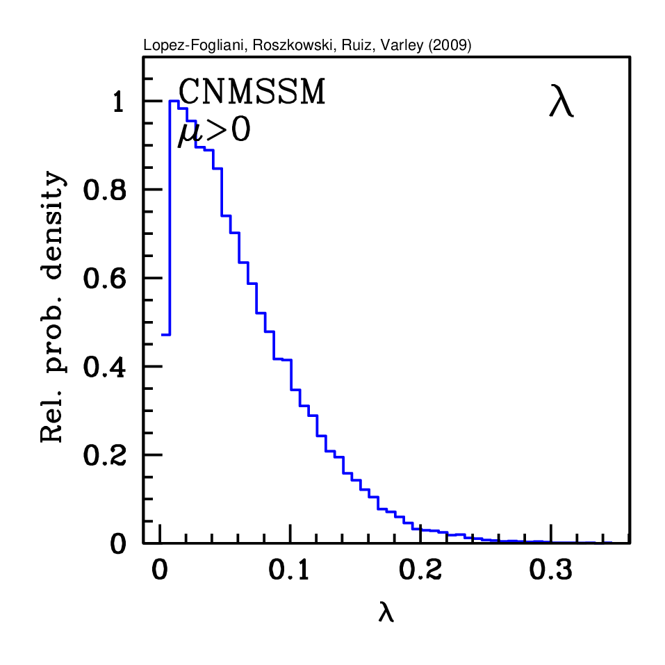
It is also instructive to show 2D probability maps of the effective parameter vs. some of the CNMSSM parameters. This is presented in Fig. 4. We can see that the consistency of the model and the applied set of constraints favor below some , the range comparable to , as expected. In other words, in the CNMSSM the problem is solved without any need for additional fine tuning of parameters. We can also see an interesting correlation with but not with the other C(N)MSSM parameters. This is caused primarily by the CP-odd Higgs funnel effect and the fact that its mass is correlated with . These features are presented in Fig. 5. Finally, in Fig. 6 we present 1D pdfs of several key parameters which show more clearly their high probability ranges.
 |
 |
 |
 |
 |
 |
 |
 |
Prior dependence is often an issue in Bayesian statistics and needs to be addressed. Even the CMSSM tends to be under-constrained which leads to a fairly strong prior dependence [51], and in the NUHM, with two extra parameters, the situation becomes worse [20]. In the left panel of Fig. 7 we show a 2D pdf in the () plane assuming the flat prior in all the CNMSSM parameters. By comparing with the analogous panel of Fig. 1 we indeed see a substantial shift in the high probability region to larger values, as typical for the flat prior due to the volume effect.
A related issues is that of the assumed range of input parameters. We have already seen in the left panel of Fig. 7 that was not well confined to the assumed range below . In order to examine this, in the right panel of Fig. 7 we show a 2D pdf in the () plane with greatly extended ranges of both parameters () and taking the log prior. Clearly, there is basically no cap on the 95% total probability range in both parameters, although of course such large values of soft mass parameters can hardly be considered as well motivated in effective low-energy SUSY models.
 |
 |
 |
 |
 |
 |
We have already emphasized that the high probability regions of the crucial parameters and in the CNMSSM are quite similar to the well studied CMSSM case. One of the key features of the CMSSM is that the neutralino LSP is mostly a bino, except for the FP region of large , where a larger admixture of the higgsino is present. In the CNMSSM, with an additional singlet field whose mass is controlled by , the picture could in principle be very different from the CMSSM. We examine this in Fig. 8 where we separately show the regions where the LSP is mostly gaugino () (left panel), doublet higgsino () (middle left panel), the mixed region ( and ) (middle right panel), as well as mostly singlino () (right panel). (The wino component is always negligible and below we will show only the bino fraction .) We can see that in an overwhelming fraction of cases the LSP still remains predominantly bino-like. This is in agreement with the panel showing in Fig. 6 where small values of the product tend to be strongly disfavored. We expose those non-CMSSM like cases in Fig. 9. Clearly, points corresponding to singlino LSP cases exist but are rare.


Similarly to the CMSSM, the key observables shaping the high probability regions of the model are: , , and the light Higgs mass . Their 1D pdfs are presented in Fig. 10. We can see that, apart from , they reproduce the likelihood rather well, especially for our default log prior (long-dashed red curve), although even for the flat prior the fit is not bad, except for , again with much resemblance to the CMSSM [51].
The sharp cutoff in at the LEP limit results from the approximation that we have adopted, as mentioned above. Given the complexities of the Higgs sector and a much larger list of possible decay channels, we have taken an approximate approach of setting the likelihood to one or zero for points that are accepted or excluded by LEP data using the NMSPEC code. A more correct would would have allowed for some “tail” at lower masses, as in the CMSSM [17], and would have expanded allowed ranges of and towards smaller values but this would have a limited effect on this analysis in which we are mostly interested in presenting mainly global features of the CNMSSM. Nevertheless, it is worth stressing that in an exploratory run with the LEP limit smeared out we have found only a few points for which the singlet component is barely enough to escape the limit of . In this sense we expect that a full analysis would have basically reproduced the case of the CMSSM [17].
 |
 |
 |
 |
The Higgs sector of the NMSSM contains three CP-even bosons , and , two CP-odd ones and , as well as a pair of the charged Higgs . Fig. 11 shows the relative 1D pdfs of (left panel), (middle panel) and (right panel) for both our default log prior (long-dashed red) and the flat prior (dotted blue) for comparison. We can see that the prior dependence is not very strong, with the flat prior favoring larger values, as usual. Also, by comparing with Fig. 5 of Ref. [17], we can see that the pdfs are quite similar to the analogous states in the CMSSM.
 |
 |
 |
In Fig. 12 we present the relative 1D pdfs for several superpartners, in a fashion similar to the previous Figure. Again, we can see that the log prior gives somewhat lower ranges of masses, especially for the scalars, which primarily depend on and that the distributions are rather similar to the corresponding ones in the CMSSM; compare, eg, Fig. 17 of Ref. [16]. It is clear that there will be a rather mixed chance of detecting those states at the LHC. For example, with the gluino to be probed up to some , nearly the whole range will be tested with the log prior, but much less so with the flat prior. The scalars, on the other hand, will be much more challenging for both priors.
In Table 4 we list the best fit values for a number of observables for our default log prior and also, for comparison, for the flat prior. We stress, however, that the log prior appears more appropriate for exploring unified low-energy SUSY models, as already emphasized above.
| Parameter | Best fit (log) | Best fit (flat) |
|---|---|---|
| 101 GeV | 478 GeV | |
| 404 GeV | 632 GeV | |
| -165 GeV | 1.20 TeV | |
| 12.9 | 42.4 | |
| 0.009 | 0.0252 | |
| 547 GeV | 672 GeV | |
| 274 GeV | 476 GeV | |
| 0.093 | 0.094 | |
| 114.4 GeV | 114.3 GeV | |
| 164 GeV | 263 GeV | |
| 309 GeV | 491 GeV | |
| 950 GeV | 1.45 TeV | |
| 9.6965 | 9.4635 |
 |
 |
 |
 |
 |
 |
Finally, we move to discussing the model’s predictions for the detection of the lightest neutralino assumed to be the DM in the Universe in direct detection searches via its elastic scatterings with targets in underground detectors. We follow the same procedure and formalism as previously in [16, 18, 51]. The underlying formalism can be found in several sources, e.g., in Refs. [55, 54, 56, 57].
In Fig. 13 we present the 2D posterior pdfs in the usual plane spanned by the spin-independent cross section and the neutralino mass . The left (right) panel corresponds to the log (flat) prior. For comparison, some of the most stringent 90% CL experimental upper limits are also marked [44, 45, 46, 47, 48, 49], although they have not been imposed in the likelihood, as before in our studies of the CMSSM, because of substantial astrophysical uncertainties, especially in the figure for the local density.
Several key features can be seen in Fig. 13. Firstly, the prior dependence is not very strong for both 68% and 95% total probability regions, which is encouraging. It does not affect much the banana-shape high-probability region which corresponds to the Higgs funnel and the stau coannihilation regions. The horizontal branch of is more affected because it corresponds to the focus point region of large . Next, the overall shape rather closely resembles the case of the CMSSM, see, e.g., Fig. 18 of Ref. [51] or Fig. 13 of Ref. [16]. (The slight upwards shift in results from changing the code from DarkSusy to Micromegas.) It does, on the other hand, differ from the predictions of the NUHM which features an additional higgsino-like region at ; see Fig. 12 of Ref. [20].
Independently of the prior, basically the whole 68% and 95% total probability regions are likely to be within the planned reach of of future 1-tonne detectors. Some of the currently operating detectors are already probing some of the high probability regions, and with a “modest” improvement down to , they will be testing some of the most likely cross sections.
 |
 |
V Conclusions and summary
The Next-to-Minimal Supersymmetric Standard Model solves the -problem of the MSSM but, without grand unification, both models suffer from a large number of parameters. The constrained versions of both models are in this respect much more well-motivated. Because of the additional singlet superfield present in the CNMSSM, the resulting phenomenology in the Higgs and neutralino sectors is considerably richer. Therefore, a prior one could expect that the models could be distinguished in experimental tests.
The global exploration of wide ranges of CNMSSM parameters and a Bayesian analysis show that, from the statistical point of view, this is not the case. The coupling strongly favors as small values as possible, in other words it tends towards the decoupling regime in which one recovers the CMSSM plus the basically decoupled singlet Higgs and the singlino. As a result, Higgs and superpartner mass spectra also tend to resemble those of the CMSSM, as does the cross section for direct detection of neutralino dark matter. Nevertheless, we have identified a limited number of cases where the LSP is indeed singlino-dominated, but statistically they are not very significant.
In conclusion, the CNMSSM is, for the most part, testable at the LHC and in dark matter searches, which is certainly encouraging. On the other hand, should a CMSSM-like signal be detected, it is likely to be very challenging to distinguish between the two models.
Acknowledgments
LR is partially supported by the EC 6th
Framework Programmes MRTN-CT-2004-503369 and MRTN-CT-2006-035505.
RRdA is supported by the project PARSIFAL (FPA2007-60323) of the
Ministerio de Educación y Ciencia of Spain. DL-F and TV are supported by
STFC. The use of the Iceberg computer cluster at the
University of Sheffield is gratefully acknowledged. LR would like to
thank the CERN Theory Division for hospitality during the final stages
of the project.
References
- [1]
See, e.g., H. E. Haber and G. L. Kane,
The Search for Supersymmetry: Probing Physics Beyond the Standard Mode
l
Phys. Rep.117198575;
S. P. Martin, A Supersymmetry Primer, hep-ph/9709356. - [2] G. L. Kane, C. F. Kolda, L. Roszkowski and J. D. Wells, Study of constrained minimal supersymmetry, Phys. Rev. D4919946173 [hep-ph/9312272].
- [3] J.E. Kim and H.P. Nilles, The problem and the strong CP problem, Phys. Lett. B 138 (1984) 150.
- [4]
P. Fayet,
Supergauge invariant extension of the Higgs mechanism and a model for the electron and its neutrino, J. High Energy Phys. B 901975104;
R. K. Kaul and P. Majumdar, Cancellation of quadratically divergent mass corrections in globally supersymmetric spontaneously broken gauge theories, Nucl. Phys. B 199 (1982) 36;
R. Barbieri, S. Ferrara and C. A. Savoy, Gauge models with spontaneously broken local supersymmetry, Phys. Lett. B 119 (1982) 343;
H. P. Nilles, M. Srednicki and D. Wyler, Weak interaction breakdown induced by supergravity, Phys. Lett. B 120 (1984) 346;
J. M. Frere, D. R. T. Jones and S. Raby, Fermion masses and induction of the weak scale by supergravity, Nucl. Phys. B 222 (1983) 11;
J. P. Derendinger and C. A. Savoy, Quantum effects and SU(2)U(1) breaking in supergravity gauge theories, Nucl. Phys. B 237 (1984) 307. - [5] G. F. Giudice and A. Masiero, A Natural Solution to the mu Problem in Supergravity Theories., Phys. Lett. B2064801988.
- [6]
J. R. Ellis, J. F. Gunion, H. E. Haber, L. Roszkowski and F. Zwirner,
Higgs bosons in a nonminimal supersymmetric model, Phys. Rev. D 39 (1989) 844;
M. Drees, Supersymmetric models with extended Higgs sector, Int. J. Mod. Phys. A 4 (1989) 3635;
U. Ellwanger, M. Rausch de Traubenberg and C. A. Savoy, Particle spectrum in supersymmetric models with a gauge singlet, Phys. Lett. B 315 (1993) 331 [arXiv:hep-ph/9307322]; Phenomenology of supersymmetric models with a singlet, Nucl. Phys. B 492 (1997) 21 [arXiv:hep-ph/9611251];
S. F. King and P. L. White, Resolving the constrained minimal and next-to-minimal supersymmetric standard models, Phys. Rev. D 52 (1995) 4183 [arXiv:hep-ph/9505326]. - [7] U. Ellwanger and C. Hugonie, Topologies of the (M+1)SSM with a singlino LSP at LEP2, Eur. Phys. J. C 13 (2000) 681 [arXiv:hep-ph/9812427].
- [8] U. Ellwanger, J. F. Gunion, C. Hugonie and S. Moretti, NMSSM Higgs discovery at the LHC, arXiv:hep-ph/0401228.
- [9] U. Ellwanger and C. Hugonie, Masses and couplings of the lightest Higgs bosons in the (M+1)SSM, Eur. Phys. J. C 25 (2002) 297 [arXiv:hep-ph/9909260].
- [10] U. Ellwanger, J. F. Gunion and C. Hugonie, NMHDECAY: A Fortran code for the Higgs masses, couplings and decay widths in the NMSSM, arXiv:hep-ph/0406215.
- [11] S. A. Abel, S. Sarkar and P. L. White, On the cosmological domain wall problem for the minimally extended supersymmetric standard model, Nucl. Phys. B 454 (1995) 663 [arXiv:hep-ph/9506359].
- [12]
S. A. Abel,
Destabilising divergences in the NMSSM, Nucl. Phys. B480 (1996) 55 [arXiv:hep-ph/9609323].
- [13]
H. P. Nilles, M. Srednicki and D. Wyler, Constraints on the
stability of mass hierarchies in supergravity Phys. Lett. B124
(1983) 337;
C. Panagiotakopoulos and K. Tamvakis, Stabilized NMSSM without domain walls, Phys. Lett. B446 (1999) 224 [arXiv:hep-ph/9809475]. - [14]
T. Elliott, S. F. King and P. L. White, Phys. Lett. B 351 (1995) 213 [arXiv:hep-ph/9406303];
U. Ellwanger, M. Rausch de Traubenberg and C. A. Savoy,Phys. Lett. B 315 (1993) 331 [arXiv:hep-ph/9307322], Z. Phys. C 67 (1995) 665 [arXiv:hep-ph/9502206] and Nucl. Phys. B 492 (1997) 21 [arXiv:hep-ph/9611251];
S. F. King and P. L. White, Phys. Rev. D 52 (1995) 4183 [arXiv:hep-ph/9505326];
U. Ellwanger and C. Hugonie, Eur. Phys. J. C 25 (2002) 297 [arXiv:hep-ph/9909260]. - [15] Ulrich Ellwanger and Cyril Hugonie, NMSPEC: A Fortran code for the sparticle and Higgs masses in the NMSSM with GUT scale boundary conditions, Published in Comput. Phys. Commun. 177 (2007) [arXiv:hep-ph/0612134].
- [16] R. Ruiz de Austri, R. Trotta and L. Roszkowski, A Markov Chain Monte Carlo analysis of the CMSSM, J. High Energy Phys. 06052006002 [hep-ph/0602028]; see also R. Trotta, R. Ruiz de Austri and L. Roszkowski, Prospects for direct dark matter detection in the Constrained MSSM, [astro-ph/0609126].
- [17] L. Roszkowski, R. Ruiz de Austri and R. Trotta, On the detectability of the CMSSM light Higgs boson at the Tevatron, J. High Energy Phys. 07042007084 [hep-ph/0611173].
- [18] L. Roszkowski, R. Ruiz de Austri and R. Trotta, Implications for the Constrained MSSM from a new prediction for b to s gamma, J. High Energy Phys. 07072007075 [hep-ph/0705.2012].
- [19]
B. C. Allanach and C. G. Lester,
Multi-dimensional MSUGRA likelihood maps,
Phys. Rev. D732006015013 [hep-ph/0507283];
B. C. Allanach, Naturalness priors and fits to the constrained minimal supersymmetric standard model, Phys. Lett. B6352006123 [hep-ph/0601089];
B. C. Allanach, C. G. Lester and A. M. Weber, The dark side of mSUGRA, J. High Energy Phys. 06122006065 [hep-ph/0609295]. - [20] L. Roszkowski, R. Ruiz de Austri, R. Trotta, S. Tsai and T. Varley, Some novel features of the Non-Universal Higgs Model, arXiv:0903.1279.
- [21] F. Feroz, B. C. Allanach, M. Hobson, S. S. AbdusSalam, R. Trotta and A. M. Weber, Bayesian Selection of sign(mu) within mSUGRA in Global Fits Including WMAP5 Results, J. High Energy Phys. 102008064.
- [22] S. S. AbdusSalam, B. C. Allanach, F. Quevedo, F. Feroz, M. Hobson, Fitting the Phenomenological MSSM, arXiv:0904.2548.
- [23] C. F. Berger, J. S. Gainer, J. L. Hewett, T. G. Rizzo, Supersymmetry Without Prejudice, arXiv:0812.0980.
- [24] Benjamin C. Allanach, Fernando Quevedo, Kerim Suruliz, Low-energy supersymmetry breaking from string flux compactifications: Benchmark scenarios, J. High Energy Phys. 06042006040 [arXiv:hep-ph/0512081].
- [25] B. C. Allanach, M. J. Dolan and A. M. Weber, Global Fits of the Large Volume String Scenario to WMAP5 and Other Indirect Constraints Using Markov Chain Monte Carlo, J. High Energy Phys. 08082008105 [arXiv:0806.1184 [hep-ph].
- [26] http://www.th.u-psud.fr/NMHDECAY/nmssmtools.html
- [27] G. Belanger, F. Boudjema, A. Pukhov and A. Semenov, MicrOMEGAs: A program for calculating the relic density in the MSSM, Comput. Phys. Commun. 149 (2002) 103 [hep-ph/0112278]; MicrOMEGAs: Version 1.3, Comput. Phys. Commun. 174, 577 (2006) [hep-ph/0405253].
- [28] D. G. Cerdeño, C. Hugonie, D. E. López-Fogliani, C. Muñoz and A. M. Teixeira, Theoretical predictions for the direct detection of neutralino dark matter in the NMSSM, J. High Energy Phys. 04122004048 [arXiv:hep-ph/0408102].
- [29]
Florian Domingo and Ulrich Ellwanger, Constraints from the Muon g-2 on the Parameter Space of the NMSSM, J. High Energy Phys. 08072008079 arXiv:0806.0733 [hep-ph];
C. Hugonie, G. Belanger, A. Pukhov. Dark matter in the constrained NMSSM, JCAP 0711 (2007) 009 arXiv:0707.0628 [hep-ph];
G. Belanger, C. Hugonie and A. Pukhov, Precision measurements, dark matter direct detection and LHC Higgs searches in a constrained NMSSM JCAP 0901 (2009) 023, arXiv:0811.3224 [hep-ph]. - [30] R. Flores, K.A. Olive and D. Thomas, Light-neutralino interactions in matter in an extended supersymmetric standard model, Phys. Lett. B 263 (1991) 425.
- [31] M. Bastero-Gil, C. Hugonie, S. F. King, D. P. Roy and S. Vempati, Does LEP prefer the NMSSM?, Phys. Lett. B 489 (2000) 359 [arXiv:hep-ph/0006198].
- [32] V.A. Bednyakov and H.V. Klapdor-Kleingrothaus, About direct dark matter detection in next-to-minimal supersymmetric standard model, Phys. Rev. D 59 (1999) 023514 [arXiv:hep-ph/9802344].
- [33]
B.R. Greene and P.J. Miron,
Supersymmetric cosmology with a gauge singlet, Phys. Lett. B 168 (1986) 226;
R. Flores, K.A. Olive and D. Thomas, A new dark matter candidate in the minimal extension of the supersymmetric standard model, Phys. Lett. B 245 (1990) 509;
K.A. Olive and D. Thomas, A light dark matter candidate in an extended supersymmetric model, Nucl. Phys. B 355 (1991) 192;
S.A. Abel, S. Sarkar and I.B. Whittingham, Neutralino dark matter in a class of unified theories, Nucl. Phys. B 392 (1993) 83 [arXiv:hep-ph/9209292];
A. Stephan, Dark matter constraints on the parameter space and particle spectra in the nonminimal SUSY standard model, Phys. Lett. B 411 (1997) 97 [arXiv:hep-ph/9704232]; Dark matter constraints in the minimal and nonminimal SUSY standard model, Phys. Rev. D 58 (1998) 035011 [arXiv:hep-ph/9709262];
A. Menon, D. E. Morrissey and C. E. M. Wagner, Electroweak baryogenesis and dark matter in the nMSSM, [arXiv:hep-ph/0404184].
U. Ellwanger,Nonrenormalizable interactions from supergravity, quantum corrections and effective low-energy theories, Phys. Lett. B 133 (1983) 187;
J. Bagger and E. Poppitz, Destabilizing divergences in supergravity coupled supersymmetric theories, Phys. Rev. Lett. 71 (1993) 2380 [arXiv:hep-ph/9307317];
J. Bagger, E. Poppitz and L. Randall, Destabilizing divergences in supergravity theories at two loops, Nucl. Phys. B 455 (1995) 59 [arXiv:hep-ph/9505244]. - [34] By CDF Collaboration and D0 Collaboration, A Combination of CDF and D0 Results on the Mass of the Top Quark arXiv:0803.1683 [hep-ex].
- [35] W.-M. Yao et al., The Review of Particle Physics, J. Phys. G 33 (2006) 1 and 2007 partial update for the 2008 edition.
- [36] See http://lepewwg.web.cern.ch/LEPEWWG.
- [37] J. P. Miller, E. de Rafael and B. L. Roberts, Muon g-2: Review of Theory and Experiment, Rept. Prog. Phys. 70 (2007) 795 [arXiv:hep-ph/0703049].
- [38] The CDF Collaboration, Measurement of the oscillation frequency, Phys. Rev. Lett. 97 (2006) 062003 [hep-ex/0606027]; and Observation of oscillations, Phys. Rev. Lett. 97 (2006) 242003 [hep-ex/0609040].
- [39] J. Dunkley et al. [The WMAP Collaboration], Five-year Wilkinson Microwave Anisotropy Probe (WMAP) Observations: Likelihoods and parameters from the WMAP data, arXiv:0803.0586 [astro-ph].
- [40] The CDF Collaboration, Search for and decays in collisions with CDF-II, CDF note 8956 (August 2007).
- [41] The LEP Higgs Working Group, http://lephiggs.web.cern.ch/LEPHIGGS; G. Abbiendi et al. [the ALEPH Collaboration, the DELPHI Collaboration, the L3 Collaboration and the OPAL Collaboration, The LEP Working Group for Higgs Boson Searches], Search for the standard model Higgs boson at LEP, Phys. Lett. B 565 (2003) 61 [hep-ex/0306033].
- [42] K. L. Chan, U. Chattopadhyay and P. Nath, Naturalness, weak scale supersymmetry and the prospect for the observation of supersymmetry at the Tevatron and at the LHC, Phys. Rev. D581998096004 [hep-ph9710473].
- [43] J. L. Feng, K. T. Matchev and T. Moroi, Multi - TeV scalars are natural in minimal supergravity, Phys. Rev. Lett. 8420002322 [hep-ph/9908309] and Focus points and naturalness in supersymmetry, Phys. Rev. D612000075005 [hep-ph9909334].
- [44] The CDMS Collaboration, Limits on spin–independent WIMP-nucleon interactions from the two-tower run of the Cryogenic Dark Matter Search, Phys. Rev. Lett. 962006011302 [astro-ph/0509259].
- [45] V. Sanglard et al.[EDELWEISS Collaboration], Final results of the EDELWEISS–I dark matter search with cryogenic heat–and–ionization Ge detectors, Phys. Rev. D712005122002 [astro-ph/0503265].
- [46] G. J. Alner et al.[UK Dark Matter Collaboration], First limits on nuclear recoil events from the ZEPLIN–I galactic dark matter detector, Astropart. Phys.232005444.
- [47] G. J. Alner et al., First limits on WIMP nuclear recoil signals in ZEPLIN-II: A two phas e xenon detector for dark matter detection, Astropart. Phys. 28 (2007) 287 [astro-ph/0701858].
- [48] V. N. Lebedenko et al., Result from the First Science Run of the ZEPLIN-III Dark Matter Sear ch Experiment, arXiv:0812.1150 [astro-ph].
- [49] J. Angle et al. [XENON Collaboration], First Results from the XENON10 Dark Matter Experiment at the Gran Sa sso National Laboratory Phys. Rev. Lett. 100 (2008) 021303 [astro-ph/0706.0039].
- [50] See: http://www.superbayes.org/
- [51] R. Trotta, F. Feroz, M. P. Hobson, L. Roszkowski and R. Ruiz de Austri, The impact of priors and observables on parameter inferences in the Constrained MSSM, J. High Energy Phys. 08122008024 [hep-ph/0809.3792].
- [52] J. Skilling, Nested sampling, in R. Fischer, R. Preuss and U. von Toussaint, (Eds.) Bayesian Inference and Maximum Entropy Methods in Science and Engineering, 735 (Amer. Inst. Phys. conf. proc. 2004), 395-405; J. Skilling, Bayesian Analysis 1, 833-861 (2006).
- [53]
F. Feroz and M. P. Hobson,
Multimodal nested sampling: an efficient and robust alternative to
MCMC methods for astronomical data analysis,
Mon. Not. Roy. Astron. Soc. 384 449 (2008);
F. Feroz, M. P. Hobson and M. Bridges, MultiNest: an efficient and robust Bayesian inference tool for cosmology and particle physics (2008), arXiv:0809.3437. - [54] See, e.g., G. Jungman, M. Kamionkowski and K. Griest, Supersymmetric dark matter, Phys. Rep.2671996195.
- [55] M. Drees and M. Nojiri, Neutralino - nucleon scattering revisited, Phys. Rev. D4819933483 (hep-ph9307208). Phys. Rev. D 48, 3483 (1993), hep-ph/9307208.
- [56] J. Ellis, A. Ferstl, K. A. Olive, Re-evaluation of the elastic scatteri ng of supersymmetric dark matter, Phys. Lett. B4812000304 [hep-ph0001005].
- [57] Y. G. Kim, T. Nihei, L. Roszkowski and R. Ruiz de Austri, Upper and lower limits on neutralino WIMP mass and spin-independent scattering cross section, and impact of new (g-2)(mu) measurement, J. High Energy Phys. 021220020342002 [hep-ph/0208069].