Dynamical Compactification and Inflation
in Einstein-Yang-Mills Theory
with Higher Derivative Coupling
Abstract
We study cosmology of the Einstein-Yang-Mills theory in ten dimensions with a quartic term in the Yang-Mills field strength. We obtain analytically a class of cosmological solutions in which the extra dimensions are static and the scale factor of the four-dimensional Friedmann-Lemaitre-Robertson-Walker metric is an exponential function of time. This means that the model can explain inflation. Then we look for solutions that describe dynamical compactification of the extra dimensions. The effective cosmological constant in the four-dimensional universe is determined from the gravitational coupling, ten-dimensional cosmological constant, gauge coupling and higher derivative coupling. By numerical integration, the solution with is found to behave as a matter-dominated universe which asymptotically approaches flat space-time, while the solution with a non-vanishing approaches de Sitter space-time in the asymptotic future.
I Introduction
There have been many attempts to consider extra dimensions in addition to our world of four-dimensional space-time, even though they have not been observed. The original idea dates back to Nordström [1], Weyl [2], Kaluza [3] and Klein [4], who considered extra dimensions in order to unify gravity and electromagnetic force in five space-time dimensions. Now the most promising unified theory, describing all fundamental forces including two types of nuclear forces, is considered to exist in ten, eleven or twelve dimensions after string theory, M-theory [5] and F-theory [6] have appeared. Superstring theory is consistent in ten-dimensional space-time. The extra six dimensions should be compactified. Some people require supersymmetry in four-dimensional space-time and the extra-dimensional space was assumed as a Calabi-Yau manifold. After the discovery of D-branes, D-branes or more generally “branes” offer the possibility of large extra dimensions or the brane-world scenario [7].
There were many efforts to describe cosmological solutions in the framework of higher-dimensional theories. Especially, the realization of de-Sitter like expansion of a 4-dimensional part has attracted much attention in connection with the inflationary scenario or the current accelerated expansion of our universe. One of those attempts is the flux compactification, which have received a lot of attention in recent years [8]. One of the most important and basic features of the flux compactification is to stabilize the size of a compactified space by certain configurations of high-rank differential form fields.
Before string theory was discovered, Cremmer and Scherk studied an attractive possibility of compactification with the size of a compactified space being stabilized [9]. In order to achieve it they placed a non-trivial topological solution (soliton) of a gauge field on the compactified space, for instance a monopole on the sphere or a Yang-Mills instanton on the four-dimensional sphere . In these cases, the compactified space is stabilized at a finite radius rather than decompactified to an infinite radius. So they called it “spontaneous compactification”.
In this paper we would like to study if such a compactification can occur dynamically or not. In general, in order to stabilize a topological configuration of a Yang-Mills field in dimensions greater than four, we need higher order terms of the gauge field strength [10]. Some years ago Tchrakian introduced such a term, which we call the Tchrakian term, in order to generalize ’t Hooft-Polyakov monopoles and Yang-Mills instantons to those analogues in dimensions greater than four [11]. The term is not renormalizable, but still quadratic in the time derivative. Recently some of the present authors have numerically studied a monopole-like solution in six-dimensional Minkowski space by adding the Tchrakian term [12].11 1 This was originally motivated by the computation of non-Abelian Berry’s phases in T-dualized USp matrix model [13]. One of the authors has further studied asymptotic solution of five-dimensional Tchrakian monopole, the generalization of Tchrakian monopole [14]. In the case of a six-dimensional sphere, an exact solution to a generalized self-duality relation has been constructed for SO(6) Yang-Mills fields with the Tchrakian term [15].22 2 Generalization of instantons on the complex projective space has been also given [16]. Then this relation has been successfully embedded in the Einstein-Yang-Mills theory with the Tchrakian term in the geometry of the direct product of the four-dimensional Minkowski space (anti-de Sitter space AdS4) and of a constant radius, with (without) a ten-dimensional cosmological constant [17]. In this solution the gauge field distributes on homogeneously, so it is a natural generalization of Cremmer and Scherk [9]. At least for the Yang-Mills part, the configuration attains the minimum of the Bogomol’nyi bound when the radius of satisfies a certain relation with the gauge coupling constant and the coupling strength of the Tchrakian term. Therefore we expect that if we turn on the time variation of the space-time, we obtain a solution which describes the process of dynamical compactification.
In this paper we consider cosmological solutions with a time-dependent scale factor of the three dimensions as well as with a time-dependent radius of , and study if there exist solutions with the radius of tending to a finite value, as a possible model of dynamical compactification.
This paper is organized as follows. In Sec. II, we describe our theory, that is, the Einstein-Yang-Mills theory with the Tchrakian term in ten dimensions. We review the discussion of Bogomol’nyi completion. In Sec. III, we introduce an ansatz on the ten-dimensional metric, namely, the direct product of the four-dimensional Friedmann-Lemaitre-Robertson-Walker (FLRW) metric and with the radius as a function of time. Then we specify a gauge configuration which satisfies the self-duality relation and solves the Yang-Mills equation with the Tchrakian term. In Sec. IV, simple analytical solutions with a fixed radius of are given. The four-dimensional part of the solutions is either Minkowski or de Sitter, depending on the choice of the model parameters. In Sec. V, we consider solutions that describe the process of dynamical compactification. We investigate the behavior of the solutions both analytically and numerically. In general, the four-dimensional part behaves as de Sitter plus small oscillations, while the radius undergoes damped oscillations toward a finite value. For a particular choice of the model parameters that gives the product of a flat space-time times with a fixed radius, we find the four-dimensional part behaves as a dust-dominated universe, that is, with the scale factor proportional to . Sec. VI is devoted to conclusion and discussions.
II Model Setting and Bogomol’nyi Equation
Let us start from the following action in ten-dimensional space-time:
| (1) | ||||
| (2) | ||||
| (3) |
Here is the invariant volume form, is the scalar curvature with respect to the metric and is the field strength two-form which takes values in the Lie algebra so(6). The star () denotes the Hodge dual operator acting on differential forms in ten dimensions. Our notation is summarized in Appendix A. For more details, see [18].
We consider the case where the space-time is locally a product space of and . is a four-dimensional curved space-time and is a compact space. Let us denote the total space . Metric on this space is
| (4) | ||||
| (5) |
For the case where the field strength has only components along the compact directions, we can manipulate the Yang-Mills action as [17]
| (6) | ||||
| (7) | ||||
| (8) |
where represents the Hodge dual operator along the compact direction . We call this procedure Bogomol’nyi completion. The term is a surface term and it gives the bound on the energy density. Then the Bogomol’nyi equation is
| (9) |
If either of these equations is satisfied, the energy attains the minimum given by irrespective of the sign .
Suppose that is a solution of equation of motion and is the corresponding field strength. We denote the fluctuations around this solution , . Let us expand the left hand side of Eq. (9) in terms of these fluctuations:
| (10) |
where
| (11) | ||||
| (12) | ||||
| (13) | ||||
| (14) |
Here is the zero-th order term with respect to . The term is linear in . The remaining includes higher order terms. By substituting this to Eq. (8), we obtain
| (15) | |||
| (16) | |||
| (17) |
Here the term is a total derivative term because is a solution of the equation of motion. The term includes indefinite quadratic form of , which might yield a tachyonic mass term. When is a solution of which is one of Eq. (9), no tachyonic mass term appears in gauge sector. We mention that this does not necessarily mean the stability of the system under the presence of fluctuations of both the metric and the gauge field. This is an issue to be studied in the future.
III Ansatz for the metric and gauge fields
In this section we consider time-dependent solutions in the sense of Freund [19]. Namely, the metric is assumed to be in the form,
| (18) | ||||
| (19) |
where the coordinates span the three-dimensional space and span . and . The parameter is or . and are functions of time . is a constant with dimension of length. The radius of is given by . This type of metrics was considered in various contexts, for instance in [20, 21].
The SO(6) gauge field configuration, represented in terms of differential forms, is assumed to be in the form,
| (20) |
where are the indices of the Lie algebra of SO(6), are the infinitesimal generators represented by spinor, and is the vielbein of the six dimensional metric ,
| (21) |
is the gauge coupling constant. In the configuration of the gauge field , the internal indices and the spatial indices are identified by an embedding of the spin connection of the six-dimensional sphere into the gauge group.
The exterior derivatives of the vielbeins are
| (22) | ||||
| (23) |
Then the Ricci tensor components are given by
| (24) | ||||
| (25) | ||||
| (26) |
The scalar curvature is
| (27) |
Thus the Einstein tensor components are given by
| (28) | ||||
| (29) | ||||
| (30) |
As for the gauge field, its field strength is given by
| (31) |
This satisfies the following duality relations,
| (32) |
where
| (33) |
The self duality relation Eq. (32) becomes the Bogomol’nyi equation (9) if . In this case, there are no tachyonic modes at least in gauge sector. This determines a particular radius of the extra dimensions in terms of the gauge coupling constants and ,
| (34) |
Because depends only on the time coordinate, the exterior derivative of vanishes,
| (35) |
This means that the configuration satisfies the equation of motion,
| (36) |
The energy momentum tensor of the gauge field is given by
| (37) | ||||
| (38) |
Here are the components of introduced in Appendix A. For our gauge configuration we have
| (39) | |||||
| (40) |
where
| (41) |
In this gauge configuration, the Einstein field equations are
| (42) | |||
| (43) | |||
| (44) | |||
| (45) |
where the first equation is a constraint on the field and its derivatives, the Hamiltonian constraint equation, determining the three-dimensional hypersurface in the four-dimensional phase space. We note that the kinetic term in the Hamiltonian constraint is quadratic in the field velocities, and it has one positive and one negative eigenvalues. The above system of differential equations is invariant under the time translation and time reversal transformation. If , there is in addition an invariance under the shift of . The time evolution of the fields and is determined by Eqs. (43) and (45), describing the trajectory on the three-dimensional hypersurface defined by the constraint equation.
It is convenient to express the field equations in terms of a rescaled time coordinate , and introduce the following dimensionless parameters,
| (46) | ||||
| (47) | ||||
| (48) |
where is related to the ten-dimensional cosmological constant by . In what follow, the -derivative of a function will be denoted by . For the parameter is fixed to the value , leaving only two free parameters in the field equations.
By manipulating the field equations we can reduce them to the following convenient set of two differential equations:
| (49) | ||||
| (50) |
where and are defined by
| (51) | ||||
| (52) | ||||
| (53) |
We can solve Eq. (49) for to obtain
| (54) |
By using this equation, we can eliminate from Eq. (50). Then the Einstein field equations are reduced to a system of coupled differential equations given by
| (55) | ||||
| (56) |
where we have chosen the positive value of the square root in Eq. (55). In the next section, we look for a solution in which the extra-dimensional part of the metric is static, that is, a solution with . In this case, grows with time for the above choice of the square root sign, ensuring that the four-dimensional part of the metric describes an expanding universe.
IV Solutions with static extra dimensions
In this section we consider solutions in which the metric of the extra dimensional space, , is static, that is when constant. In this case, Eq. (55) becomes integrable with respect to , and Eq. (56) becomes an algebraic equation for . We note that we do not require our solution to satisfy the Bogomol’nyi equation (9). Hence for those solutions whose extra-dimensional radius is different from given by Eq. (34), the absence of tachyon modes is not guaranteed. Therefore we simply assume that there is a sufficiently wide range of parameters in which there appears no harmful tachyons. This issue is left for a future study.
Below we first consider general solutions. As we will see shortly, there is a particular solution given by for . Since this is somehow special, we treat it separately.
IV.1 The general case
Static solutions of Eq. (56) are determined by the roots of . Let us set . We note that , where is the linear scale of the extra dimensions. The equation becomes
| (57) |
where
| (58) |
Note that and are independent of and . As demonstrated in Appendix B, the equation has one or two real solutions and (we assume ) provided that and satisfy a certain inequality.
Let us first consider the solution . The relation between the original variables and can be written as
| (59) |
where represents the size of the extra dimensions. Thus the size of the extra dimensions is completely fixed by the coupling constants.
As easily seen, Eqs. (55) and (56) are invariant under the rescaling,
| (60) |
Using this degree of freedom, we fix the length scale to be the size of the extra dimensions , or equivalently, we set for this solution. Then we have . Therefore must be a solution of Eq. (57):
| (61) |
With this normalization, we find a positive real for . The condition and give the following inequalities:
| (62) |
In terms of these two solutions are given by
| (63) |
Those points are critical points or equilibrium solutions of the differential equation (56). The value of is depicted as a function of for each value of in Fig. 1. The discussions in the rest of this subsection is valid for both solutions.

Now we turn to Eq. (55). Setting , we have
| (64) |
where () is defined by
| (65) |
We assume is positive. gives an additional condition on the parameter ,
| (66) |
If this inequality is satisfied, , because is concave downward as a function of and its derivative at is negative. The allowed region of and given by Eq. (66) is depicted in Fig. 2.

The equation (64) can be integrated to give
| (67) |
where the origin of the time coordinate has been chosen to make the expression simple. Four-dimensional parts of these solutions are the same as those of Ishihara [20].
For large , the term proportional to can be neglected and the scale factor of the four-dimensional space-time approaches , which describes a universe with accelerated expansion. Thus, although we do not claim that our model can give a realistic model of the universe, depending on the value of the constant , it can reproduce a period of inflation in the very early universe or the present universe dominated by a very small cosmological constant.
IV.2 The case
When the solution (67) is no longer valid as it is, and we need a special treatment. In this case Eq. (64) implies that must be either or . In either case, , and the solution is
| (68) |
where is an integration constant.
The four-dimensional part of the solution for is flat. It was obtained in [17], which is almost the same as the one obtained by Cremmer-Scherk [9], but with the radius of and the value of ten-dimensional cosmological constant modified by the presence of the Tchrakian term.
The solution for is also flat. The four dimensional line element is
| (69) |
This metric covers the inside of either the future light cone or the past light cone of the flat space-time.
V Dynamical Compactification
In this section, we switch on the time dependence of in order to see if our model has the possibility to describe the process of dynamical compactification. For this purpose, we analyze the stability of the solution () and in the second order nonlinear differential equation (56) in the case of both analytically and numerically.
We first analyze the stability of the critical points analytically. For this purpose, we linearize the system of differential equations (see e.g. [22]). We find, however, that for this method is not sufficient to establish the stability of the critical point . Therefore we will try a different approach in this case.
We first consider the critical point , which is a stationary or equilibrium solution of the differential equation (56). Denoting and and keeping only terms linear in and , Eq. (56) is written as the following system of first order differential equations:
where the matrix is given by
with
| (78) | ||||
| (79) |
Note that in the above is equal to the one defined by Eq. (65) with the normalization condition (61). The solution is asymptotically stable if both of the two eigenvalues of the matrix ,
| (80) |
have negative real part.
To analyze the stability of the second critical point, , we simply replace by when linearizing Eq. (56). Then the eigenvalues are
| (81) |
For the real part of the two eigenvalues is zero, and the linear system corresponds to the harmonic oscillator for . In this case we can not apply Poincare-Lyapunov’s theorem above and additional information is required to establish the character of the critical point for the full nonlinear equation. We therefore treat this case separately.
V.1 The case
As in Sec. IV, we are interested in the solutions with real and positive. Then the real part of the eigenvalues is negative if
| (82) |
This condition coincides with the condition , which is satisfied when the parameters satisfy Eq. (66). Thus the critical point is stable.
The system shows two different kinds of behavior in the neighborhood of the critical point . When , the system undergoes damped oscillations with the amplitude decreasing as . Otherwise the system is over-damped, showing simple exponential damping toward the critical point.
For the second critical point , it can be shown that
| (83) |
where is the function introduced in Eq. (57) and is the solution of corresponding to the second critical point. This inequality follows from the fact that is a monotonically increasing function of with the unique at and , which is proved in Appendix B. If , there are two real eigenvalues with opposite signs. Hence the critical point is an unstable saddle-point. In the special case when , the first and second critical points become degenerate, and becomes the only equilibrium solution of the system. Note that we have in this case.
To confirm the above stability analysis, we have performed numerical integration of Eq. (56). Our numerical results indicate that the linear analysis around the first critical point is accurate. In Fig. 3, we show the phase-space orbits of the solutions of Eq. (56) with . In this case, the first critical point is stable and the other critical point along the axis is an unstable saddle point. The location of the saddle point depends on the values of the parameters and as well, and it roughly defines an effective stability radius for orbits near the solution . The time evolution of for an asymptotically stable solution is shown in Fig. 7, where oscillates with a decreasing amplitude until reaches zero.
We have also integrated Eq. (55) for . The time evolution of the three-dimensional cosmic scale factor is shown in Fig. 5. Initially when the oscillatory energy of is non-negligible, the scale factor behaves as the one in a matter-dominated universe, . For sufficiently large , after the amplitude of has decayed exponentially, the universe eventually enters a stage of accelerated expansion, , with the (dimensionless) Hubble parameter .


V.2 The case
In the case the real part of is zero, rendering the linear analysis insufficient to determine the stability of the solution. Therefore we have to take into account the second order terms.
To second order in and , Eq. (56) gives the equations,
| (84) | ||||
| (85) |
where is a quadratic function given by
| (86) |
Let us solve Eqs. (84) and (85) perturbatively. We assume . To first order in and , the system describes a harmonic oscillator. Namely we have
| (87) | ||||
| (88) |
as a solution of the first order equations, where and are arbitrary constants. Then the orbits in phase-space are ellipses about the critical point .
Now we consider the effect of the second order terms. Here we just apply the so-called Krylov-Bogoliubov method of averaging [22] to study the behavior of the solutions.33 3 Detailed calculation is shown in Appendix C.
First, we introduce varying constants in the harmonic oscillator solution as
| (89) | ||||
| (90) |
Then the system of differential equations may be expressed as
| (91) | ||||
| (92) |
where
| (93) | ||||
| (94) |
Note that the right-hand sides of Eqs. (91) and (92) are periodic in with the period . Then instead of these equations, applying the Krylov-Bogoliubov method of averaging we consider the time-averaged equations:
| (95) | ||||
| (96) |
for and . The solution is given by
| (97) | ||||
| (98) |
These give approximate behavior of and at sufficiently large . From Eq. (89), approximations to and for large are given by
| (99) | ||||
| (100) |
Then, for large , Eq. (55) gives
| (101) |
We can now read off an approximate solution for the field ,
| (102) |
Thus the scale factor behaves as
| (103) |
Apart from the small oscillations, this describes a matter-dominated universe.
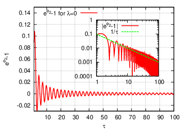
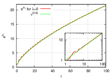
In Figs. 6-7, we show numerical solutions of the full non-linear system for . The numerical results are in good agreement with our analytical estimations. The time evolution of in Fig. 7 clearly exhibits oscillations around its central value as we have shown analytically.
VI Conclusion and Discussion
In this article, we studied time-dependent solutions of the ten-dimensional Einstein-Yang-Mills theory with the Tchrakian term. We obtained a class of simple analytic solutions in which the extra dimensions are static and the scale factor of the four-dimensional Friedmann-Lemaitre-Robertson-Walker metric behaves exponentially in time with the rate of expansion given by constants denoted by (). Thus our model admits solutions describing inflation.
We then considered a possible dynamical compactification of the extra dimensions by allowing them to be time-dependent. In the case , we found solutions in which the scale factor of the extra dimensions undergoes damped oscillations and approaches a constant value, while the four-dimensional scale factor approaches . In the case of , we found numerically that the scale factor behaves as a matter-dominated universe .
Our model includes four dimensionful constants . They define four typical length scales in our model. Or if we fix the Planck scale or the gravitational constant, , we are left with three dimensionless parameters. In addition, if we require the Bogomol’nyi equation to be satisfied, the linear size of the extra dimensions is fixed to be , and there remains only two dimensionless parameters.
As is shown in Sec. II, when the radius of the compact direction is equal to , there are no tachyonic mode in the gauge sector. However, for a set of model parameters that gives a radius substantially different from , a tachyonic mode may appear. To investigate when a tachyon appears and how it affects our model is certainly an important issue. Also for a complete analysis, in addition to fluctuations of the gauge field, it is necessary to include fluctuations of the metric and cross terms between them. These are left for future work.
We also note that all the discussions given in this paper applies equally to the gauge group SU(4) in place of SO(6), because the matrices are block diagonalizable. Namely, if we project those matrices on the four-dimensional eigenspace with respect to the eigenvalue of , we obtain self-duality relation of SU(4) without . Thus all cosmological solutions obtained in this paper are also valid for models with SU(4) gauge theory. Furthermore, since SU(4) is a subgroup of SU(), our cosmological solutions can be embedded into the Einstein-Yang-Mills theory with the Tchrakian term with SU() gauge group. Generalization to other gauge groups like or SO() with remains as a future issue [23].
Recently some of us (HK and MN) considered the Bogomol’nyi equation on [16]. By using the gauge configuration on , we expect that we will be able to obtain similar cosmological solutions for compactification instead of studied in this paper. Also, it is interesting to see if similar cosmological solutions can be obtained for other types of compactification such as the compactification in terms of the Casimir energy [24]. These are also issues to be investigated in the future.
Acknowledgements.
HK would like to show his appreciation to Sung-Jay Lee, Qing-Guo Huang, Pravabati Chingangbam and Eoin Ó Colgáin for their advises. HK thanks to H. Emoto for his comments. HK and MS thank KIAS and its members, particularly Ki-Myeong Lee and Piljin Yi, for their hospitality. The work of MN is supported in part by Grant-in-Aid for Scientific Research No. 20740141 of Monbukagaku-sho (MEXT). The work of MS is supported in part by JSPS Grant-in-Aid for Scientific Research (A) No. 21244033, and by JSPS Grant-in-Aid for Creative Scientific Research No. 19GS0219, and by MEXT Grant-in-Aid for the global COE program at Kyoto University, ”The Next Generation of Physics, Spun from Universality and Emergence”.Appendix A Notation
A.1 Definitions and Properties of Tensors
Here we explain our notation. The Einstein tensor and the energy momentum tensor are defined as
| (104) |
In terms of these tensors the Einstein equation is
| (105) |
The Einstein tensor is obtained by the differentiation of the Einstein-Hilbert action with respect to the metric . The corresponding Levi-Civita connection is defined as
| (106) |
The Riemannian curvature is defined as
| (107) |
The Ricci tensor and scalar curvature are
| (108) |
A.2 Differential Forms
The tangent vector space of a point is spanned by . The basis of the cotangent space is the dual vector, . For vector space the Grassmann algebra is defined as where is the tensor algebra and is the two-sided ideal generated by . We can define a linear operation which is called the Hodge dual. Let us fix and . The Hodge dual operator is defined as
| (109) |
By using the Hodge dual operation the metric on the differential Suppose that is a -form,
| (110) |
The inner product is given by . Let us show the metric in terms of the component,
| (111) | ||||
| (112) | ||||
| (113) | ||||
| (114) |
where the metric is defined as follows:
| (115) |
Here is the -th symmetric group consisting of all permutations of characters. Finally we obtain
| (116) |
The minus sign is from the fact that the signature of the metric is Lorentzian.
A.3 Clifford algebra
We will use the Clifford algebra with respect to the six-dimensional Euclidean metric in order to represent the algebra so(6). Indices refer to the inner space. The Clifford algebra is generated by which satisfy
| (117) |
These generators are represented as matrices. satisfy the commutation relation of the Lie algebra so(6). Anticommutation relation of is
| (118) |
Here is an antisymmetric product of four generators defined as
| (119) |
The chirality operator is defined as
| (120) |
By using this matrix, is written as a sum of products of and ,
| (121) |
A.4 Notation for Gauge Fields
The degree of freedom of a gauge boson is represented by the Lie algebra-valued one-form ,
| (122) |
where is the corresponding gauge field strength two-form and is the gauge coupling constant. Let us rewrite the action in terms of the components,
| (123) | ||||
| (124) | ||||
| (125) | ||||
| (126) |
For notational simplicity, we introduce the composite four form operator ,
| (127) |
The energy momentum tensor is
| (128) | ||||
| (129) |
where
| (130) |
Appendix B constant solutions
In this Appendix, we derive an inequality which gives the condition for Eq. (57) to have two real solutions.
Because for arbitrary , the polynomial has a unique minimum. This means that the number of real solutions of , Eq. (57), is at most 2. Let the value of at the minimum be . Then must be non-positive for a real solution to exist:
| (131) |
Also must be the unique real solution of the equation,
| (132) |
Because is negative, must be positive. In fact, by using Cardano’s formula, we obtain
| (133) |
which is manifestly positive definite.
Now using , the condition (131) reduces to
| (134) |
Thus when the couplings satisfy the condition (134), there are one or two real solutions and , (). Because is positive, and we have the relation , is always positive if it exists. When the equality in Eq. (134) is satisfied, we have .
We assume that the parameters satisfy Eq. (134). Then for or equivalently , we have , hence both solutions are non-negative: . The solutions are given by the Ferrari’s formula,
| (135) |
Here and are , and is
| (136) |
where
| (137) |
If and satisfy Eq. (134), . This means that is positive. The equation must have only one or two real solutions. This implies because if . Thus the two real solutions are
| (138) |
where .
The above expressions for the solutions and are quite complicated as they are. However, using the scaling freedom of , it is possible to simplify the expressions. For this purpose, let us first recapitulate Eq. (59) where the length representing the linear extension of the extra dimensions was introduced,
| (139) |
Then we set , which implies .
Also for , we may also simplify the expression in terms of with the normalization . In this case, since is a solution of , we have Eq. (61),
| (140) |
and can be divided by . The quotient is
| (141) |
In order to use the Cardano’s formula, let us change the equation into the normal form,
| (142) |
where
| (143) |
This equation has only one real positive solution . Therefore the solution is
| (144) |
Finally let us derive the bounds on the parameters and . We assume . From Eq. (140), this gives a bound on and ,
| (145) |
In addition, since Eq. (141) has only one real positive solution which is equal to or smaller than , the left-hand side of it is non-negative at ,
| (146) |
Therefore the conditions that and yield the bounds on the parameters and as
| (147) |
Appendix C Asymptotic behavior in the case of
Here we derive the asymptotic behavior of the solution of the system given by Eqs. (84) and (85). Equations (91) and (92) can be written as
| (148) | |||||
| (149) |
By eliminating the term from these equations, we obtain
| (150) |
where
| (151) |
We can integrate this to obtain an expression for ,
| (152) |
As for the angle , from Eqs. (149) and (150), it satisfies
| (153) |
As clear from this equation, tends to a constant for , Then will be a function oscillating around zero. This implies that the integral of in Eq. (150) cannot be large. Thus in the region where is large enough, damps out in time as ,
| (154) |
This is consistent with our anticipation that tends to a constant. Therefore ignoring an irrelevant integration constant, the asymptotic behaviors of and at large are given by
| (155) |
References
- [1] G. Nordstrom, Phys. Z. 15 (1914) 504 [arXiv:physics/0702221].
- [2] H. Weyl, Sitzungsber. Preuss. Akad. Wiss. Berlin (Math. Phys. ) 1918 (1918) 465.
- [3] T. Kaluza, Sitzungsber. Preuss. Akad. Wiss. Berlin (Math. Phys. ) 1921 (1921) 966.
- [4] O. Klein, Z. Phys. 37 (1926) 895 [Surveys High Energ. Phys. 5 (1986) 241].
- [5] E. Witten, Nucl. Phys. B 443, 85 (1995) [arXiv:hep-th/9503124].
- [6] C. Vafa, Nucl. Phys. B 469, 403 (1996) [arXiv:hep-th/9602022].
- [7] N. Arkani-Hamed, S. Dimopoulos and G. R. Dvali, Phys. Lett. B 429, 263 (1998) [arXiv:hep-ph/9803315]; L. Randall and R. Sundrum, Phys. Rev. Lett. 83, 3370 (1999) [arXiv:hep-ph/9905221]; Phys. Rev. Lett. 83, 4690 (1999) [arXiv:hep-th/9906064].
- [8] S. Kachru, R. Kallosh, A. Linde, J. M. Maldacena, L. P. McAllister and S. P. Trivedi, JCAP 0310, 013 (2003) [arXiv:hep-th/0308055]. S. Kachru, R. Kallosh, A. Linde, J. M. Maldacena, L. P. McAllister and S. P. Trivedi, JCAP 0310, 013 (2003) [arXiv:hep-th/0308055]. S. Kachru, R. Kallosh, A. Linde and S. P. Trivedi, Phys. Rev. D 68, 046005 (2003) [arXiv:hep-th/0301240];
- [9] E. Cremmer and J. Scherk, Nucl. Phys. B 108, 409 (1976); Nucl. Phys. B 118, 61 (1977).
- [10] G. H. Derrick, J. Math. Phys. 5 (1964) 1252; N. S. Manton and P. Sutcliffe, Cambridge, UK: Univ. Pr. (2004) 493 p
- [11] D. H. Tchrakian, J. Math. Phys. 21, 166 (1980); D. H. Tchrakian, Phys. Lett. B 150, 360 (1985).
- [12] H. Kihara, Y. Hosotani and M. Nitta, Phys. Rev. D 71, 041701 (2005) [arXiv:hep-th/0408068].
- [13] B. Chen, H. Itoyama and H. Kihara, Mod. Phys. Lett. A 14, 869 (1999) [arXiv:hep-th/9810237]; Nucl. Phys. B 577, 23 (2000) [arXiv:hep-th/9909075].
- [14] H. Kihara, Phys. Rev. D 77, 127703 (2008) [arXiv:0802.3244 [hep-th]]; Phys. Rev. D 79, 045021 (2009) [arXiv:0810.4750 [hep-th]].
- [15] H. Kihara and M. Nitta, Phys. Rev. D 77, 047702 (2008) [arXiv:hep-th/0703166].
- [16] H. Kihara and M. Nitta, J. Math. Phys. 50, 012301 (2009) [arXiv:0807.1259 [hep-th]].
- [17] H. Kihara and M. Nitta, Phys. Rev. D 76, 085001 (2007) [arXiv:0704.0505 [hep-th]].
- [18] T. Eguchi, P. B. Gilkey and A. J. Hanson, Phys. Rept. 66, 213 (1980).
- [19] P. G. O. Freund, Nucl. Phys. B 209, 146 (1982).
- [20] H. Ishihara, Prog. Theor. Phys. 72, 376 (1984). H. Ishihara, Phys. Lett. B 179, 217 (1986).
- [21] H. Nariai, “On The Electromagnetic Waves In A Peculiar Universe With The Topology S(2) X S(2),” RRK-86-10, (1986).
- [22] P. Smith, D. Jordan, D. W. Jordan, “Nonlinear Ordinary Differential Equations: An Introduction for Scientists and Engineers,” Oxford University Press, New York, 1977
- [23] H. Kihara and E. Ó Colgáin, arXiv:0906.4610 [hep-th].
- [24] S. M. Carroll, M. C. Johnson and L. Randall, arXiv:0904.3115 [hep-th]; F. R. Klinkhamer, arXiv:0904.3276 [gr-qc]. B. R. Greene and J. Levin, JHEP 0711, 096 (2007) [arXiv:0707.1062 [hep-th]]; C. Csaki, M. Graesser, L. Randall and J. Terning, Phys. Rev. D 62, 045015 (2000) [arXiv:hep-ph/9911406]; F. Ferrer and S. Rasanen, JHEP 0602, 016 (2006) [arXiv:hep-th/0509225]; F. Ferrer, T. Multamaki and S. Rasanen, JHEP 0904, 006 (2009) [arXiv:0812.4182 [hep-th]].