Percolation thresholds on 2D Voronoi networks and Delaunay triangulations
Abstract
The site percolation threshold for the random Voronoi network is determined numerically for the first time, with the result , using Monte-Carlo simulation on periodic systems of up to 40000 sites. The result is very close to the recent theoretical estimate of Neher, Mecke, and Wagner. For the bond threshold on the Voronoi network, we find , implying that for its dual, the Delaunay triangulation, . These results rule out the conjecture by Hsu and Huang that the bond thresholds are 2/3 and 1/3 respectively, but support the conjecture of Wierman that for fully triangulated lattices other than the regular triangular lattice, the bond threshold is less than .
I Introduction
The Voronoi diagram [1] for a given set of points on a plane (Fig. 1) is simple to define. Given some set of points on a plane , the Voronoi diagram divides the plane into polygons, each containing exactly one member of . Each point’s polygon cordons off the portion of that is closer to that point than to any other member of . More precisely, the Voronoi polygon around contains all locations on that are closer to than to any other element of . The total Voronoi diagram is the set of all the Voronoi polygons for on ; the Voronoi network is the set of vertices and edges of the Voronoi diagram.
The dual to the Voronoi diagram is interesting in its own right. Known as the Delaunay triangulation [2] (see Fig. 2), it can be defined independently of the Voronoi diagram for the same set of points on : it is simply the set of all possible triangles formed from triples chosen out of whose circumscribed circles do not contain any other members of (Fig. 3). The Delaunay triangulation and the Voronoi diagram for the same set of points can be seen in Fig. 4. Note that while the members of are sites in the Delaunay triangulation, they are not sites in the Voronoi network, whose sites are the vertices of the polygons; also note that the edges of the Voronoi diagram lie along the perpendicular bisectors of the edges of the Delaunay triangulation — however, the edges of the Voronoi diagram do not always intersect the edges of the Delaunay triangulation, as seen in Fig. 4. The Delaunay triangulation represents the connectivity of the Voronoi tessellation of the surface.
There are many algorithms for constructing these networks. The fastest ones run in time for general distributions of points [3, 4, 5, 6], where is the number of generating sites, and this has been proven to be the optimal worst-case performance [4]. For a Poisson distribution of points on the plane, there are many expected-time algorithms [7, 8, 9, 10].
In addition to being theoretically interesting [11, 12, 13, 14, 15], both the Voronoi diagram and the Delaunay triangulation are widely used in modeling and analyzing physical systems. They have seen use in lattice field theory and gauge theories [16], analyzing molecular dynamics of glassy liquids [17], detecting galaxy clusters [18], modeling the atomic structure and folding of proteins [19, 20], modeling plant ecosystems and plant epidemiology [21], solving wireless signal routing problems [22, 23], assisting with peer-to-peer (P2P) network construction [24], the finite-element method of solving differential equations [25], game theory [26, 27], modeling fragmentation [28], and numerous other areas [29, 30].
Percolation theory is used to describe a wide variety of natural phenomena [31, 32]. In the nearly seventy years since the first papers on percolation appeared [33, 34], it has become a paradigmatic example of a continuous phase transition. For a given network, finding the critical probability, , at which the percolation transition occurs is a problem of particular interest. has been found analytically for certain 2D networks [35, 36, 37]; however, most networks remain analytically intractable. Numerical methods have been used to find for many such networks, e.g., [31, 38, 39, 40, 41, 42, 43].
In this paper we consider the percolation thresholds of the Voronoi and Delaunay networks for a Poisson distribution of generating points, as represented in Figs. 1, 2, and 4. There are four percolation thresholds related to these two networks: the site and bond percolation on each. Being a fully triangulated network, the site percolation threshold of the Delaunay network is exactly [35, 44, 45, 46]. This result has recently been proven rigorously by Bollobás and Riordan [47]. Somewhat surprisingly, a search of the literature revealed no prior calculation of the site percolation threshold of the Voronoi network at all, despite the widespread use of such networks. A prediction for its value has recently been made by Neher, Mecke and Wagner [48]; they use an empirical formula to predict , but they too were unable to find any previous calculation of this value, either analytically or numerically. (There are places in the literature (e.g. [29]) where the Voronoi “site” threshold is listed as 1/2. This is true if the “sites” are taken to be the generating points from which the diagram is created, rather than the vertices of the diagram. Thus, this is actually the Voronoi tiling threshold, i.e. the percolation threshold of the Voronoi polygons, which is in turn equivalent to the Delaunay site threshold, well known to be 1/2.)
The bond thresholds of the Voronoi and Delaunay networks are complementary,
| (1) |
because these networks are dual to one another [49]. The first numerical measurement of the bond threshold for either network seems to be that of Jerauld et al. [50], who in 1984 found . Shortly thereafter, Yuge and Hori [51] performed a renormalization group calculation which yielded . In 1999, Hsu and Huang [52] found and through Monte Carlo methods. (The numbers in parentheses represent the errors in the last digits.) These values led them to make the intriguing conjecture that the thresholds are exactly and respectively. There is, however, no known theoretical reason to believe that this conjecture is true. In order to test this conjecture, and to find the site percolation threshold of the Voronoi network, we have carried out extensive numerical simulations, as detailed below. In section II, we describe our methods, and in section III we discuss our results and compare them to the thresholds of several related lattices, and also discuss the covering graph and further generalizations of the Voronoi system. Conclusions are given in section IV.
II Generating algorithms and analysis techniques
II.1 Delaunay/Voronoi generation algorithm
In order to avoid edge effects in the networks when growing percolation clusters, and to make it possible to use more sites as seeds for those clusters (see subsection II.2), we wished to create Voronoi and Delaunay networks with periodic boundary conditions. While popular fast algorithms for generating Voronoi and Delaunay networks exist, most notably the Quickhull algorithm [53], these do not generally support periodic boundary conditions. We therefore created our own fairly straightforward algorithm for generating the desired networks. After coming up with it independently, we later found that it falls into the class of expected-linear-time algorithms known as Incremental Search [8]. The basic outline of the algorithm is as follows:
- 1.
Divide the region in which the generating points (vertices of the Delaunay triangulation) are located into squares of equal size (“bins”).
- 2.
Find a single Delaunay edge by picking a point at random and searching through its bin and neighboring bins to find the point which is its nearest neighbor.
- 3.
Given a Delaunay edge and a “side” to look on (immediately above or below the edge), determine the third point in the Delaunay triangle by looking at the radii of the circumcircles of the triangles formed by that edge with each point in its bin and all of the neighboring bins.
- 4.
Look at the other Delaunay triangles that have been found in that bin and neighboring bins to make sure this new triangle is not a duplicate of one that has already been found. If it is not, find which of its neighbors have already been discovered and mark them as its neighbors, and vice versa.
- 5.
From the list of neighbors of the current triangle, figure out which of its edges are not already shared with neighbors (if any), and, if there are any unshared edges, whether the missing neighbor should be above or below the edge.
- 6.
Repeat steps 3-5 until there are no unprocessed edges left, at which point the Delaunay triangulation is finished. Because the neighbors of each triangle are known, this algorithm also yields an adjacency list of the sites on the Voronoi diagram (because the Voronoi diagram is dual to the Delaunay triangulation).
This algorithm is significantly easier to implement with periodic boundary conditions, because every triangle is guaranteed to have exactly three neighbors. Furthermore, the imposition of periodic boundary conditions also gives the Delaunay and Voronoi networks a very useful property: there are always exactly twice as many Delaunay triangles (Voronoi sites) as there are generating points (vertices of the Delaunay network or polygons in the Voronoi network) for a given diagram. This is a consequence of the more general fact that that the number of faces (triangles) must be double the number of vertices (sites) for any fully triangulated network with doubly-periodic boundary conditions in two dimensions. This fact follows from Euler’s formula and is proven in the appendix. This simple relation makes it easier to spot certain kinds of errors in the code, because improperly written code is rather unlikely to consistently produce the proper number of sites for the given number of generating points. Using this algorithm, we generated thousands of Voronoi diagrams of 40,000 sites each. Fig. 5 shows an example of a smaller Delaunay triangulation created with this algorithm.
II.2 Percolation cluster growth and finding
The Leath-type epidemic growth method [54] that we used involves growing a large number of percolation clusters in order to find . For site percolation clusters, we start with a seed site somewhere on the network. Each of its neighbors is turned on with probability or off with probability . Neighbors of active sites are then visited and the procedure is repeated for all their previously unvisited neighbors; the cluster either dies out naturally or is stopped by the program when it hits a cutoff size of 1000 sites. For bond percolation clusters, an analogous algorithm is used in which sites are simply never turned off, as it is the bonds between sites that are pertinent.
Due to the fact that our Voronoi diagrams are finite and are generated from a random Poisson distribution of points, each diagram yields a slightly different effective value of ; therefore, we had to generate many diagrams. This could have been very computationally expensive, but the choice of periodic boundary conditions helped here as well. Because there are no edges to the diagrams, we were able to place the seed point for a cluster at any site on a diagram, rather than being limited to a small subset of sites near the center. This meant we were able to use many widely separated seed points to grow clusters on each diagram, which reduced the impact of each seed point’s immediate neighborhood upon the value of obtained for each diagram. This, in turn, dramatically reduced the number of distinct diagrams we needed to obtain a particular level of precision. Specifically, we grew clusters of up to 1000 sites on each of 800 diagrams, for a total of clusters grown at each value of . We then repeated this process at each of various near to generate the plots in the next section. Finally, this process was done twice — once for site percolation and once for bond percolation, both on the Voronoi network.
Because the percolation clusters are cut off before they can become large enough to wrap around the network, the clusters effectively see the diagram as infinite in size. Thus, their size distribution can be used to obtain an unbiased estimate of , the probability that a percolation cluster will grow to be at least size (for ) on an infinite network. At the critical threshold , as , where for the two-dimensional percolation cluster universality class [31]. (It is expected that the critical exponents here are the same as for regular two-dimensional lattices.) In the scaling region, where is large and is small such that is constant (with ), behaves as
| (2) |
where and are non-universal metric constants specific to the system being considered, and is a universal scaling function analytic about . If we operate close to such that , then we can make a Taylor-series expansion of to find
| (3) |
where is another constant. Thus, plotting vs. should yield a straight line at large when is near , and that line will have a slope of zero when . Fig. 6 shows several such plots for site percolation clusters on the Voronoi network, and Fig. 7 shows several plots for bond percolation clusters on the same. does indeed approach a linear function for large in these plots, albeit far more quickly for bond percolation than for site percolation, with and .
Unfortunately, for smaller there are deviations in due to finite-size effects, and these are quite apparent for site percolation, even at the largest values of we were able to investigate. Exactly at , one expects
| (4) |
as , where is a constant and is the corrections-to-scaling exponent [55]. Similar deviations should occur when is close to . In the case of site percolation on the Voronoi network, these finite-size effects make it difficult to determine when has a truly horizontal asymptote; thus, it is not possible to use the above method to find to much greater precision than four digits when .
The most straightforward way to solve this problem would be to grow larger site percolation clusters, using a larger system to insure that wrap-around does not occur. However, because of the computational time that would be required to do that, we instead used a more sensitive method to find that takes the finite-size corrections in (4) into account.
Eq. (4) implies that, at , to leading order. This means it’s possible to estimate directly from [55]
| (5) |
Thus, in the regime where is small enough that the finite-size effects of (4) matter, yet large enough that higher-order corrections are unimportant, should approach a constant when . When , there will be deviations due to scaling. Plots of vs. for several values of can be seen in Fig. 9; these yield the result for found in the following section.
III Results and comparison with related lattices
III.1 for site and bond percolation on the Voronoi diagram
Examining Fig. 9, it can be seen that approaches a constant for large for , and we conclude
| (6) |
where the error bars are meant to indicate one standard deviation of error. This plot also gives us a rough value of 0.65 for — close to the value of found for the Penrose rhomb quasi-lattice [55].
We used the method of plotting vs. , outlined in the previous section, to find the bond percolation threshold of the Voronoi diagram. Taking the results shown in Figs. 7 and 8, we see immediately that . Because finite-size effects were not significant for bond percolation, we were able to find excellent least-squares linear fits to the asymptotic portions of the curves in Fig. 8. By plotting the slopes of these lines against the values of used (see Fig. 10), we were able to solve for the value of that would yield a slope of zero; this should be . This technique yielded a more accurate estimate:
| (7) |
which by (1) implies . We considered various contributions to the stated error. First of all, it is unclear precisely where the linear regime begins in Fig. 8, and this leads to some uncertainty in the slopes we measured from the best-fit lines. Statistical effects of course are a source of error. However, a somewhat larger source of uncertainty turned out to be the error involved in reusing the same diagram multiple times during cluster growth — even with different seed points, there is a distinct likelihood that the same part of the non-uniform diagram will be sampled. To estimate this error, we considered our usual runs of 800,000 samples on 10 different diagrams at and looked at the variation in the curves of vs. (Fig. 11). In contrast, we also looked at 10 runs of 800,000 samples each on the same diagram, to gauge the purely statistical error. We found the errors in the previous case larger than in the latter. Using the measured standard deviation and dividing by for the runs we actually used in our simulations for each value of , we estimate a final error of in the slopes of , as indicated in the error bars of Fig. 10. Finally, because the slope of the fitted line in Fig. 10 (which equals the coefficient in Eq. (3)) is nearly , we estimate that the final error in is . Note that the runs for the five values of were each done on 800 different diagrams, so there is no systematic error among the least-squares fit lines drawn in Fig. 8. Because of this, we believe our error bars are conservative.
The results for the thresholds are summarized in Table 1 and discussed further below.
| network | |||
|---|---|---|---|
| Voronoi | 3 | 0.71410(2) | 0.666931(5) |
| Delaunay | 6 (avg.) | 0.5 (exact) | 0.333069(2) |
III.2 Comparison with thresholds of related lattices
The Voronoi network has a uniform coordination number equal to 3. In Table 2, we compare the site and bond thresholds of the Voronoi diagram with several other lattices with , listed in descending order of threshold values. In the Grünbaum-Shepard notation, describes a lattice with triangles, quadrilaterals, etc., per vertex. The Archimedean lattices , , and are illustrated in [57, 56, 58]. The martini lattice was introduced in [59] and can be represented by (3/4)(3, ) + (1/4) .
We also list in Table 2 for each lattice the generalized filling factor , defined as [56]
| (8) |
which generalizes Scher and Zallen’s definition of for lattices not necessarily composed of regular polygons [60]. The has been shown to provide a good correlation to site percolation thresholds for a variety of lattices. To calculate for the Voronoi network, we use , , etc., from [61], where is the fraction of -sided polygons in the system, satisfying and for .
In Table 2 also list the fluctuations in the number of the sides of the polygons for each lattice,
| (9) |
which is equal to the fluctuations in the coordination number of the dual lattice. It follows from Euler’s formula that the average number of sides of the polygons, , in any 3-coordinated network is exactly six. For the Voronoi diagram, is known exactly as an integral [62, 61, 63].
| lattice | ||||
|---|---|---|---|---|
| 0.5 | 0.39067 | |||
| martini | 0.25 | 0.47493 | ||
| 0.222222 | 0.48601 | 0.747806a | 0.693734c | |
| 0.111111 | 0.53901 | 0.729724a | 0.676802c | |
| Voronoi | 0.049468 | 0.57351 | 0.71410e | 0.666931e |
| honeycomb | 0.0 | 0.60460 |
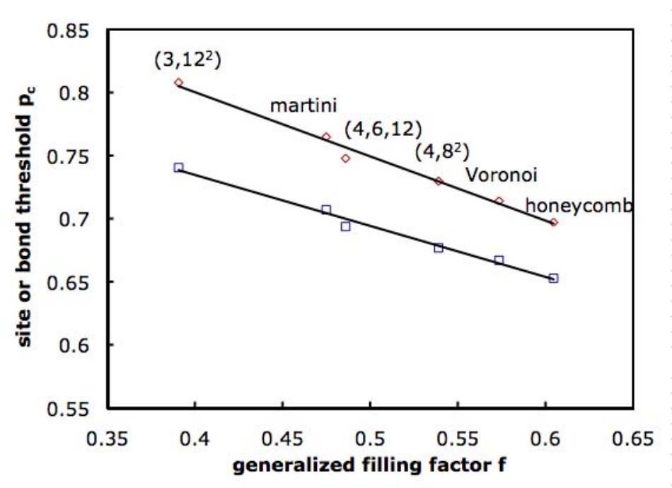
In Fig. 12 we plot the thresholds given in Table 2 as a function of . The thresholds fit well to a linear relation, as can be seen in the figure. In general, for bond percolation, is not effective in correlating thresholds, which depend strongly upon the coordination number . However, for networks with fixed , we find that the correlation of the bond thresholds with is quite good.
We can fit the linear behavior of using just data from exact results, with no numerical input. For site percolation, we use the exactly known thresholds for the (3,122) and martini lattices, while for bond percolation we use the martini and honeycomb lattice results, and find:
| (10) |
These equations imply for the Voronoi diagram (where ), and , which are evidently excellent estimates. Thus, the thresholds for the Voronoi diagram are consistent with other lattices with respect to the filling factor. A similar plot of thresholds versus the fluctuations also shows consistent behavior between the Voronoi results and those for these other lattices.
Finally, the result for the bond threshold for the Voronoi network implies the site threshold for the Voronoi covering graph, shown in Fig. 13. The covering graph (or line graph) for a given network is defined as the graph that connects the centers of the bonds together, and converts the bond percolation problem on that network to a site problem. Thus, The covering graph is a kind of randomized kagomé diagram, consisting of triangles connected together. Using similar arguments given in [67] for generalized kagomé lattices, one can find an estimate for the bond threshold of the covering lattice, with the prediction , as well as an estimate for the site-bond threshold for the Voronoi diagram. Details will be given elsewhere [68].
IV Conclusions
We have determined the site percolation threshold for the Voronoi network, for the first time and to high precision, with the result . We reiterate that this is not the well-known threshold (1/2) of the polygonal tiles of the Voronoi tessellation, which is equivalent to site percolation on the Delaunay triangulation, but rather the threshold for the 3-coordinated diagram of all the Voronoi polygons. Our Monte-Carlo result is very close to the prediction 0.7151 of Neher, Mecke and Wagner [48], and confirms their empirical procedure based upon the Euler characteristic.
We also determined the bond threshold of the Voronoi network. Our result is consistent with Jerauld et al.’s result 0.332 [50] and close to Hsu and Huang’s value 0.3333(1) [52], but runs counter to the latter authors’ conjecture that this threshold is exactly . It is interesting to note that is the value predicted by the general (approximate) bond-threshold correlation given by Vyssotsky et al. [69] for and dimension .
We made comparisons of our results with thresholds of other lattices with the same coordination number (), and found that the Voronoi thresholds are what one would expect based upon correlations with the filling factor for both the site and bond problems.
Wierman has conjectured [70] that , the bond threshold of the regular triangular lattice, is the maximum possible bond threshold for any fully triangulated network, and that no other fully triangulated network has a bond threshold greater than or equal to that value. We indeed find that the bond threshold of the fully triangulated Delaunay network is consistent with this conjecture.
For future work, it would also be interesting to look at thresholds for other random systems, such as Johnson-Mehl tessellations [71] or the graph formed by the random distribution of lines in a plane [72]. Finding thresholds in Voronoi systems of higher dimensions is another interesting open problem.
APPENDIX: Proof that for any fully triangulated network with doubly-periodic boundary conditions in two dimensions
We take advantage of the Euler relation for polyhedra to prove the desired fact about fully triangulated networks. A network on a square surface with doubly-periodic boundary conditions is topologically equivalent to placing the network on the surface of a torus; this network, in turn, can be seen as a polyhedron on the surface of the torus. Thus, the Euler relation for polyhedra applies:
where is the number of vertices on the polyhedron, is the number of edges, the number of faces, and the Euler characteristic for the 2-torus, which is zero. Because every face has exactly three edges (i.e., the network is fully triangulated), and every edge is shared by exactly two faces (the network has no boundary), we have , and we can rewrite the Euler relation as follows:
and thus . QED.
ACKNOWLEDGMENTS
This work was supported in part by the U. S. National Science Foundation Grant No. DMS-0553487.
References
- [1] G. Voronoi, J. Reine Angew. Math 134, 198 (1908).
- [2] B. Delaunay, Bulletin de l’Académie des Sciences de l’URSS, VII Serie, Class des Sciences Mathématiques et Naturelles pp. 793–800 (1934).
- [3] S. Fortune, Algorithmica 2, 153 (1987).
- [4] M. I. Shamos and D. Hoey, in Foundations of Computer Science, 1975., 16th Annual Symposium on (1975), pp. 151–162.
- [5] L. J. Guibas, D. E. Knuth, and M. Sharir, Algorithmica 7, 381 (1992).
- [6] D. T. Lee and B. J. Schachter, International Journal of Parallel Programming 9, 219 (1980).
- [7] R. A. Dwyer, Discrete and Computational Geometry 6, 343 (1991).
- [8] P. Su and S. Drysdale, in Proc. of 11th ACM Computational Geometry Conf. (1995), pp. 61–70.
- [9] A. Maus, BIT Numerical Mathematics 24, 151 (1984).
- [10] J. L. Bentley, B. W. Weide, and A. C. Yao, ACM Transactions on Mathematical Software (TOMS) 6, 563 (1980).
- [11] H. J. Hilhorst, J. Stat. Mech. Th. Exp. 2005, P09005 (2005).
- [12] H. J. Hilhorst, J. Stat. Mech. Th. Exp. 2009, P05007 (2009).
- [13] H. J. Hilhorst, Eur. Phys. J. B 64, 437 (2008).
- [14] V. Lucarini, J. Stat. Phys. 130, 1047 (2008).
- [15] M. M. de Oliveira, S. G. Alves, S. C. Ferreira, and R. Dickman, Phys. Rev. E 78, 031133 (2008).
- [16] N. H. Christ, R. Friedberg, and T. D. Lee, Nucl. Phys. B 202, 89 (1982).
- [17] F. W. Starr, S. Sastry, J. F. Douglas, and S. C. Glotzer, Phys. Rev. Lett. 89, 125501 (2002).
- [18] M. Ramella, W. Boschin, D. Fadda, and M. Nonino, Astron. Astrophys. 368, 776 (2001).
- [19] M. Gerstein, J. Tsai, and M. Levitt, J. Mol. Biol. 249, 955 (1995).
- [20] A. Poupon, Current Opinion in Structural Biology 14, 233 (2004).
- [21] O. Deussen, P. Hanrahan, B. Lintermann, R. Měch, M. Pharr, and P. Prusinkiewicz, in Proceedings of the 25th Annual Conference on Computer Graphics and Interactive Techniques (ACM New York, NY, USA, 1998), pp. 275–286.
- [22] S. Meguerdichian, F. Koushanfar, M. Potkonjak, and M. Srivastava, in IEEE INFOCOM Conference (2001), vol. 3, pp. 1380–1387.
- [23] S. Bandyopadhyay and E. Coyle, in Twenty-Second Annual Joint Conference of the IEEE Computer and Communications Societies (2003), vol. 3.
- [24] M. Naor and U. Wieder, ACM Trans. Algorithms 3, 34 (2007).
- [25] O. C. Zienkiewicz, R. L. Taylor, and J. Z. Zhu, The Finite-Element Method: Its Basis and Fundamentals (Butterworth-Heinemann, 2005).
- [26] H. K. Ahn, S. W. Cheng, O. Cheong, M. Golin, and R. van Oostrum, Theoretical Computer Science 310, 457 (2004).
- [27] O. Cheong, S. Har-Peled, N. Linial, and J. Matousek, Discrete and Computational Geometry 31, 125 (2004).
- [28] T. Kiang, Zeitschrift für Astrophysik 64, 433 (1966).
- [29] A. Okabe, B. Boots, K. Sugihara, and S. N. Chiu, Spatial Tessellations: Concepts and Applications of Voronoi Diagrams (Wiley New York, 2000), 2nd ed.
- [30] F. Aurenhammer, ACM Comput. Surv. 23, 345 (1991).
- [31] D. Stauffer and A. Aharony, Introduction to Percolation Theory (Taylor and Francis, London, 1994), 2nd ed.
- [32] M. Sahimi, Applications of Percolation Theory (Taylor & Francis, 1994).
- [33] P. J. Flory, J. Am. Chem. Soc. 63, 3083 (1941).
- [34] S. R. Broadbent and J. M. Hammersley, Proc. Camb. Phil. Soc. 53, 629 (1957).
- [35] M. F. Sykes and J. W. Essam, J. Math. Phys. 5, 1117 (1964).
- [36] J. C. Wierman, J. Phys. A 17, 1525 (1984).
- [37] R. M. Ziff and C. R. Scullard, J. Phys. A 39, 15083 (2006).
- [38] R. M. Ziff and P. N. Suding, J. Phys. A 30, 5351 (1997).
- [39] C. D. Lorenz and R. M. Ziff, J. Chem. Phys. 114, 3659 (2001).
- [40] X. Feng, Y. Deng, and H. W. J. Blöte, Phys. Rev. E 78, 031136 (2008).
- [41] S. Quintanilla, S. Torquato, and R. M. Ziff, J. Phys. A 33, L399 (2000).
- [42] H. G. Ballesteros, L. A. Fernandez, V. Martín-Mayor, A. Muñoz Sudupe, G. Parisi, and J. J. Ruiz-Lorenzo, J. Phys. A 32, 1 (1999).
- [43] P. Grassberger, Phys. Rev. E 67, 036101 (2003).
- [44] H. Kesten, Percolation Theory for Mathematicians (Birkhäuser, 1982).
- [45] M. V. Menshikov, Soviet Mathematics Doklady 33, 856 (1986).
- [46] M. Aizenman and D. J. Barsky, Comm. Math. Phys. 108, 489 (1987).
- [47] B. Bollobás and O. Riordan, Probability Theory and Related Fields 136, 417 (2006).
- [48] R. A. Neher, K. Mecke, and H. Wagner, J. Stat. Mech: Th. Exp. 2008, P01011 (2008).
- [49] B. Bollobás and O. Riordan, Random Structures and Algorithms 32, 463 (2008).
- [50] G. R. Jerauld, J. C. Hatfield, L. E. Scriven, and H. T. Davis, J. Phys. C 17, 1519 (1984).
- [51] Y. Yuge and M. Hori, J. Phys. A 19, 3665 (1986).
- [52] H.-P. Hsu and M.-C. Huang, Phys. Rev. E 60, 6361 (1999).
- [53] C. B. Barber, D. P. Dobkin, and H. Huhdanpaa, ACM Trans. Math. Softw. 22, 469 (1996).
- [54] P. L. Leath, Phys. Rev. B 14, 5046 (1976).
- [55] R. M. Ziff and F. Babalievski, Physica A 269, 201 (1999).
- [56] P. N. Suding and R. M. Ziff, Phys. Rev. E 60, 275 (1999).
- [57] B. Grünbaum and G. C. Shephard, Tilings and Patterns (Freeman, New York, 1987).
- [58] URL http://en.wikipedia.org/wiki/Percolation_threshold.
- [59] C. R. Scullard, Phys. Rev. E 73, 016107 (2006).
- [60] H. Scher and R. Zallen, J. Chem. Phys. 53, 3759 (1970).
- [61] H. J. Hilhorst, J. Phys. A 40, 2615 (2007).
- [62] K. A. Brakke, Statistics of random plane Voronoi tessellations, unpublished manuscript (1986), URL http://www.susqu.edu/brakke/aux/downloads/papers/vorplane.pdf%.
- [63] S. R. Finch, “Poisson-Voronoi tessellations,” unpublished addendum to Mathematical Constants (Cambridge: Cambridge University Press, 2003), URL http://algo.inria.fr/csolve/vi.pdf.
- [64] R. Parviainen, J. Phys. A 40, 9253 (2007).
- [65] R. M. Ziff, Phys. Rev. E 73, 016134 (2006).
- [66] M. F. Sykes and J. W. Essam, Phys. Rev. Lett. 10, 3 (1963).
- [67] R. M. Ziff and H. Gu, Phys. Rev. E 79, 020102 (2009).
- [68] R. M. Ziff and A. M. Becker (To be published).
- [69] V. A. Vyssotsky, S. B. Gordon, H. L. Frisch, and J. M. Hammersley, Phys. Rev. 123, 1566 (1961).
- [70] J. C. Wierman, J. Phys. A 35, 959 (2002).
- [71] B. Bollobás and O. Riordan, Probability Theory and Related Fields 140, 319Ð343 (2008).
- [72] S. Goudsmit, Rev. Mod. Phys. 17, 321 (1945).