A Fast and Efficient Algorithm for Slater Determinant Updates in Quantum Monte Carlo Simulations
Abstract
We present an efficient low-rank updating algorithm for updating the trial wavefunctions used in Quantum Monte Carlo (QMC) simulations. The algorithm is based on low-rank updating of the Slater determinants. In particular, the computational complexity of the algorithm is during the -th step compared with traditional algorithms that require computations, where is the system size. For single determinant trial wavefunctions the new algorithm is faster than the traditional Sherman-Morrison algorithm for up to updates. For multideterminant configuration-interaction type trial wavefunctions of determinants, the new algorithm is significantly more efficient, saving both work and storage. The algorithm enables more accurate and significantly more efficient QMC calculations using configuration interaction type wavefunctions.
I Introduction
Quantum Monte Carlo (QMC) is an approach capable of yielding highly accurate results in systems ranging from isolated molecules to the solid state[1]. The success of most common QMC methods, namely variational Monte Carlo (VMC) and diffusion Monte Carlo (DMC), depends crucially on the choice of trial wavefunction. Indeed, the trial wavefunction limits both the statistical efficiency and accuracy of the simulation. In QMC methods, the evaluation of the trial wavefunction becomes the most demanding part of the calculation especially when sufficiently large systems are considered or accurate simulations are required. This aspect of QMC was recognized even in the earliest DMC calculations, e.g. Ref. [2]. Consequently, the choice of trial wavefunction used in QMC calculations is motivated both by the accuracy and the speed of evaluation.
The most common form of trial wavefunction is of the Slater-Jastrow type
| (1) |
where, neglecting spin, is a Slater determinant, is a Jastrow function, and is a vector of the position of each electron. In QMC, the simulation commonly proceeds by proposing a local change to the electronic system configuration to . This local change in is induced by the movement of one electron at a time from position to . The probability that the proposed local change is accepted is dependent on the transition probability, which depends on the ratio of , where is a new set of electron positions. This transition probability computation in turn requires the computation of the ratio of determinants and in the new and old configurations respectively. Although a complete re-computation of can be made, an efficient algorithm that computes the necessary ratio without resorting to a complete independent calculation of each determinant can significantly increase the overall efficiency of QMC simulations. Indeed, this efficiency measure is essential to the success of Slater-Jastrow wavefunctions; for a single electron move, the conventional algorithms use Sherman-Morrison formula (special case of Sherman-Morrison-Woodbury formula [3]) which reduces the cost of evaluating to , with an cost if the move is accepted, compared with for a naive evaluation of the determinant. Once the ratio of the determinants has been calculated, most quantities required in the Monte Carlo can be obtained through a simple multiplicative scaling[1]. Comparatively recently, “linear scaling” approaches have been developed to reduce the cost of evaluating the determinants[4, 5, 6, 7, 8] by exploiting spatial locality in the studied physical system. In this paper, we explore alternative and complementary approaches to speedup the computation of transition probabilities and determinant ratios in QMC calculations.
The most accurate and commonly used QMC method is the DMC method performed in the fixed node approximation. This method exhibits a varational error in the energy depending on the quality of the nodal surfaces (zeroes) of the trail wavefunction. To improve the nodes as well as the variational quality of the trial function, it is now routine to utilize multiple determinant trial functions. These are commonly obtained from multiconfiguration quantum chemistry approaches such as the configuration interaction method where the ground state determinant is supplemented by single and double excitations from the ground state. That is,
| (2) |
where denotes a double excitation with orbitals and replaced by and respectively, and and denote the multi-determinant expansion coefficients. Higher order excitations may be progressively included. Such an expansion of the wavefunction allows the nodal surface to be improved.
There are many strong motivations for minimizing the computational cost of multideterminant wavefunctions in QMC: Recent benchmark tests of the accuracy achievable in all electron VMC utilized, for example, up to 499 determinants to obtain over 90% of the correlation energy in the first row atoms[9]. To obtain a similar fraction of correlation energy in larger systems, more determinants are likely required. Numerous recent studies [10, 11, 12] have shown the utility of increased numbers of determinants for improved accuracy in atomic, molecular, and solid-state applications. In general this result is expected since quantum chemical techniques systematically improve the wavefunction with increased numbers of determinants. Improved trial wavefunctions using multideterminants are required for large systems such as the fullerene where current trial wavefunctions are insufficient for computing accurate optical properties[13]. Multiple determinants may also be required to represent certain spin symmetries, e.g. Ref. [14]. Additionally, we have also recently shown that it is possible to sample the ground state wavefunction into a configuration expansion[15] and subsequently improve the trial wavefunction[16]. This application requires the use of large configuration interaction expansions consisting of potentially thousands of determinants.
In this paper we propose an efficient algorithm for utilizing Slater-Jastrow trial wavefunctions in QMC simulations. The algorithm is particularly efficient for multideterminant wavefunctions. Extension to related alternative wavefunction forms such as multi-pfaffian and multi-backflow wavefunctions is straightforward. In Section II we present the details of the algorithm. Section III presents benchmark timing and efficiency measures for single determinant calculations using a variety of system sizes. The multideterminant case is analysed in Section IV. Conclusions are given in Section V.
II Algorithms for updating Slater determinants
As mentioned earlier, in QMC, the Monte Carlo simulation proceeds by proposing a local change to the electronic system configuration to . The acceptance criterion for each such local change follows the traditional Metropolis algorithm, which requires the computation of the transition probability. Each time a local change is accepted, the Slater matrix is updated to by modifying one of the rows of corresponding to an electron movement from to . The simulation then proceeds by proposing a new local change, which requires the re-computation of the determinant of Slater matrix in the subsequent configuration . This progression of the simulation via local changes typically proceeds for many thousands to millions of steps until observables such as the total energy converge to a desired statistical accuracy.
The slater matrix in configuration is given by
where and for indicate respectively the spatial coordinates and spin-orbitals of -th electron. Because we are moving a single electron (say -th electron) at a time from position , the Slater matrix in the new electronic configuration is simply obtained by modifying the -th row as
The Metropolis probability to accept or reject the move is dependent on the ratio of determinants of Slater matrices , where is the determinant of Slater matrix and is the determinant of . The transition probability is in general proportional to , assuming real wavefunctions. If the move is accepted, then the system configuration changes to ; if not, the move is rejected and the system remains in configuration . In the following, whenever the context is clear, we denote by and by D.
For the Monte Carlo simulation to be efficient, all quantities related to the transition probability and any observables must be computed with minimum computational operations. In the case of a single determinant wavefunction the ratio is required. For a single electron move this corresponds to a change of a single row in the Slater matrix. However, for the case of the multideterminant wavefunction, as in Eq. 2, all ratios and are required. These ratios involve determinants with both orbital replacements and single electron moves (i.e., both row and column changes) when compared to the original ground state determinant .
For a single electron move, the basic computational problem involved during the -th MC step may be expressed as: Given the determinanat of Slater matrix , compute the determinant of such that
| (15) |
where defines an index vector that maps such that , and denotes an unit vector with on the -th entry and everywhere else. The vector corresponds to the change in Slater matrix due to the displacement of the -th electron during the -th MC step and is given by
| (16) |
A straight-forward computation of may be obtained as
| (17) |
and can be evaluated as
| (18) |
Hence, for any given , can be evaluated efficiently in computations since can be interpreted as the -th column of , i.e., . However, repetitive computation of during each of the MC simulation steps (for ) requires an efficient procedure to compute for each . For this purpose, traditional algorithms employ the Sherman-Morrison formula to update , which can be expressed as
| (19) |
Using this formula, can be updated to in computations. However, since the required number of MC steps in a typical Monte Carlo simulation readily extends to the thousands to millions range, and can increase with increasing system sizes, scaling of these traditional algorithms poses a significant hindrance for the simulation of large system sizes despite the fact that such large scale simulations are necessary to develop a better understanding of relevant chemistry and physics. As discussed in the introduction, Sec I, multiple determinants compound this problem.
Alternatively, an efficient recursive algorithm for computing may be formulated by expressing Eq. 19 as
| (20) | |||||
where and . Based on Eq. 20, a recursive scheme for computing may be formulated as
| (21) | |||||
An recursive algorithm based on Eq. 21 is presented in Algorithm 1. For each additional step , this algorithm requires storage space for two vectors and of size . In addition, we need to store an index vector that maps such that .
III Single determinant benchmarks
In order to compare the computational efficiency of the recursive algorithm with the traditional algorithm, we first tested the case of a single determinant wavefunction. An analysis of the multideterminant case is given in Sec. IV.
We tested the algorithms on a randomly generated matrix . That is, since the algorithms are applicable for general matrices, we start with a matrix whose elements are randomly chosen between zero and one. Then we consider rank-1 updates of as given by Eq. 15 for number of steps. The site locations are chosen sequentially, modulo , for these steps. The updated orbitals are chosen randomly. Figure 1 presents the ratio of the computational timings obtained using the full matrix updating and recursive updating algorithms. The timings were obtained using a standalone benchmark code using double precision arithmetic. We used the same data structures both in our recursive and full QMC simulations. Machine optimized linear algebra library calls were used for both algorithms. Timings were obtained on a 2.73 GHz Intel Xeon processor with 12 MB Cache.
Examining the timings shown in Fig. 1, we see that the recursive update algorithm is always significantly faster than the Sherman-Morrison algorithm for a small number of updates. For up to ten updates, the new algorithm times faster for a 100 sized matrix, while for a 6400 sized matrix the new algorithm is times faster. For increased numbers of updates the ratio of timings decreases. The crossover between the two algorithms occurs near the theoretically expected updates.
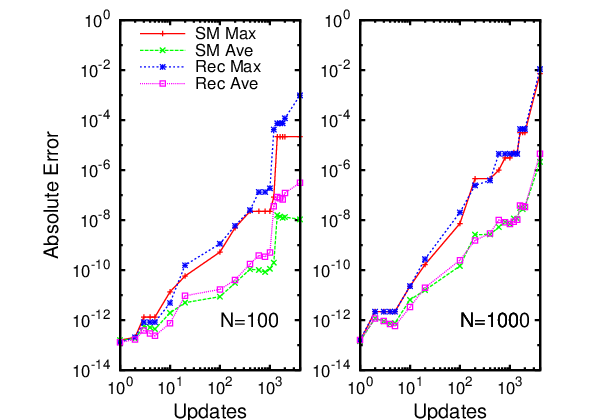
Due to the iterative nature of both algorithms numerical errors accumulate over time. It is common practise in QMC simulations to fully recalculate the inverse cofactor matrices from time to time to limit these errors. Such a recalculation requires operations. We have compared the numerical errors of the recursive update algorithm with the Sherman-Morrison algorithm and find the performance to be similar. Figure 2 illustrates the build up of errors for both algorithms for a single run.
Figure 2 shows that both algorithms have good stability and on average give high accuracy, particularly for small numbers of updates. However, for both algorithms the average and maximum numerical error in the determinant ratio gradually increases with the number of updates and can become substantial. In both cases the maximum error for a fixed number of updates can deviate by several orders of magnitude from the average. This behavior appears to be due to the occasional mixture of very small and very large numbers in the update formulae which results in a significant loss of precision. This data shows that while the recursive algorithm performs similarly to the Sherman-Morrison algorithm, it is vital to check sufficient accuracy is obtained if large numbers of updates are performed.
IV Multiple determinant wavefunctions
In the case of multiple determinant wavefunctions such as a configuration interaction expansion, all the excited Slater matrices and are similar to the ground state matrix , and differ only by a few column interchanges. The use of the recursive algorithm provides an efficient way of calculating the transition probability compared to the traditional algorithm; It is not only faster but also requires reduced storage of for storing only of the ground state matrix. No other potentially large data must be stored, although it is advantageous to reuse the current determinant values between MC steps. The recursive algorithm is used to compute the non-ground state determinants via column changes to the ground state matrix. The cost of each particle move is constant and does not increase when many steps are taken.
For simplicity we analyse the case of a multiple determinant wavefunction consisting of only the ground state determinant and determinants doubly excited from this state. Conventionally the as well as all the excited Slater matrix inverses are stored in memory to enable fastest possible update using the traditional algorithm. When the recursive algorithm is applied to multiple determinant wavefunctions, we store only the of the ground state. Conventional updates are performed on this determinant and the recursive algorithm is used to compute the other excited determinants since the excited and ground state Slater matrices differ by a few column changes. Note that successive row updates can be performed in operations using an algorithm similar to that of Algorithm 1. However, successive row updates followed by multiple column updates always requires a cost associated with a matrix-vector multiplication. Since proposed moves are usually accepted in DMC calculations with an acceptance ratio of , it is convenient to use the conventional (Sherman-Morrison) algorithm to update the inverse of the ground state Slater matrix. It should also be noted that in the event the proposed move is accepted, the traditionally updated used in the evaluation of the excited state determinants can be reused: the recursive update algorithm then requires no additional work over a single determinant calculation. Consequently, using the recursive algorithm an determinant wavefunction can be used with an updating cost scaling only linearly in and system size compared to an scaling cost using the traditional algorithm.
To evaluate determinant ratios such as we first perform a traditional update to obtain . The recursive algorithm is then used to compute from . We assume that is stored and available from a previous MC step, but this can also be calculated using two applications of the recursive algorithm to . In Table 1 we compare the costs of evaluating the determinant ratios in . Independent of the amount of storage chosen for the traditional scheme, the recursive scheme displays an improved computational cost by a factor , or times the cost of a complete single determinant update. The single determinant benchmarks of Sec. III show that these updates, which are few in number and hence correspond to the left side of Fig. 1, are several orders of magnitude faster than the traditional algorithm.
V Conclusions
In this paper, we presented an efficient low-rank updating algorithm for QMC simulations. The algorithm requires only computations during -th MC step compared with computations required by traditional algorithms. Our numerical simulations indicate that for small numbers of updates of a single determinant this algorithm is orders of magnitude faster than traditional algorithms. For single determinant wavefunctions, the traditional algorithms remain the preferred choice for more than updates. For multideterminant wavefunctions of determinants, our algorithm is the preferred choice, being significantly faster and of particular interest for large systems. In addition, it enables workspace to be reduced by a factor . The speed and storage savings of this new algorithm enables QMC calculations to use thousands of determinants.
Acknowledgment
PRCK wishes to thank F. A. Reboredo,
J. Kim, and R. Q. Hood for helpful conversations. This research is
sponsored by the Mathematical, Information and Computational Sciences
Division, Office of Advanced Scientific Computing Research and the Center for Nanophase Materials Sciences, Office of Basic Energy Sciences, both of the
U.S. Department of Energy and under contract number DE-AC05-00OR22725 with
UT-Battelle, LLC. The QMC Endstation project is supported by the
U.S. Department of Energy (DOE) under contract number DOE-DE-FG05-08OR23336.
References
- [1] W. M. C. Foulkes, L. Mitas, R. J. Needs and G. Rajagopal, Rev. Mod. Phys. 73, 33 (2001).
- [2] P. J. Reynolds, D. M. Ceperley, B. J. Alder, and W.A. Lester, J. Chem. Phys. 77, 5593 (1982).
- [3] G. H. Golub and C. F. V. Loan, Matrix Computations (The Johns Hopkins University Press, Baltimore, 1996).
- [4] A. J. Williamson, R. Q. Hood, and J. C. Grossman, Phys. Rev. Lett. 87, 246406 (2001).
- [5] F. A. Reboredo and A. J. Williamson, Phys. Rev. B 71, 121105 (2005).
- [6] D. Alfe and M. J. Gillan, Journal of Physics: Cond. Mat. 16, L305 (2004).
- [7] A. Aspuru-Guzik, R. Salomon-Ferrer, B. Austin, and W. A. Lester Jr, J. Comp. Chem. 26, 708-715 (2005).
- [8] J. Kussmann, H. Riede, and C. Ochsenfeld, Phys. Rev. B 75, 165107 (2007).
- [9] M. D. Brown, J. R. Trail, P. L. Rios, and R. J. Needs, J. Chem. Phys. 126, 224110 (2007).
- [10] J. Lawson, C. Bauschlicher, J. Toulouse, C. Filippi, and C. Umrigar, Chem. Phys. Lett. 466, 170 (2008).
- [11] J. Toulouse and C. J. Umrigar, J. Chem. Phys. 128, 174101 (2008).
- [12] J. R. Trail and R. J. Needs, J. Chem. Phys. 128, 204103 (2008).
- [13] M. L. Tiago, P. R. C. Kent, R. Q. Hood, and F. A. Reboredo, J. Chem. Phys. 129, 084311 (2008).
- [14] R. Q. Hood, P. R. C. Kent, R. J. Needs, and P. R. Briddon, Phys. Rev. Lett. 91, 076403 (2003).
- [15] F. A. Reboredo and P. R. C. Kent, Phys. Rev. B 77, 245110 (2008).
- [16] F. A. Reboredo, R. Q. Hood, and P. R. C. Kent, Accepted in Physical Review B (2009), manuscript BV10869.

| Algorithm | Move evaluation cost | Move acceptance cost | Storage cost |
|---|---|---|---|
| Traditional | |||
| Minimum storage traditional | |||
| Recursive |