Exact AdS/CFT spectrum:
Konishi dimension at any coupling

Four-dimensional Yang-Mills theories are at the heart of modern high energy physics, describing all fundamental interactions except gravity. Nevertheless, in spite of considerable efforts during almost 40 years, we still don’t have a satisfactory quantitative description of the most interesting YM theories, such as QCD, in the region of intermediate and strong couplings. The low energy quantum dynamics of YM field is mostly known only from computer simulations of lattice YM theories. A few important exact results concerned the topological, BPS sectors of N=1,2 SYM were obtained.

Recently, when the hopes on complete exact 4D solutions in particular, for the quantities given by nontrivial 4D Feynman series seemed to start waning, N=4 supersymmetric Yang-Mills theory gave us serious hopes for a better understanding of the dynamics of strongly interacting 4D gauge theories. Due to the AdS/CFT correspondence [1], as well as to the quantum integrability discovered on both sides of this duality in the planar limit (when the number of colors $N\to\infty$ with the ’t Hooft coupling $\lambda=g_{\rm YM}^{2}N$ fixed) [2, 3, 4, 5, 6, 7, 8, 9, 10, 11], we acquire little by little tools for the study of the most important quantities in N=4 SYM, such as the spectrum of dimensions $\Delta(\lambda)$ of local operators as functions of $\lambda$ - the scale independent coupling constant in this superconformal 4D theory. The weak coupling behaviour ($\lambda\to 0$) of $\Delta(\lambda)$ is given by Feynman perturbation theory. The dual string worldsheet $\sigma$-model with the coupling $g=\sqrt{\lambda}/4\pi$ allows to find the strong coupling asymptotics of various dimensions. Integrability allows us to connect the two regimes. In particular, the asymptotic Bethe ansatz (ABA) of [13] gives us the asymptotic spectrum of single trace operators containing an asymptotically large number of elementary fields.

However, for short operators, such as Konishi operator ${\rm Tr}[D,Z]^{2}$ [12] ¹¹ 1 Here $Z$ is one of the complex scalars and $D$ is a covariant derivative in a light cone direction., the calculation of anomalous dimensions is still an interesting and important challenge.

Recently we proposed the Y-system for the planar AdS/CFT [14], a set of functional equations defining the anomalous dimensions of all operators of planar N=4 SYM theory at any coupling. The integral form of the $Y$-system for excited states in $SL(2)$ sector, including the one corresponding to Konishi operator, was presented in [15]. The integral equations for the BPS vacuum energy were independently obtained in [16, 17] by the thermodynamical Bethe ansatz (TBA) technique based on the dynamics of bound states [18, 19, 20, 21, 22, 23, 24] (see also [9, 25]) of the mirror theory [26, 27]. The solutions of the integral Y-system are also solutions of the functional Y-system [16, 15, 17, 28].

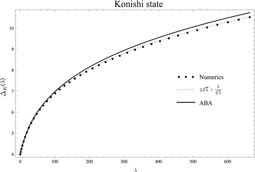
The combination of functional and integral versions of the Y-system appears to be quite efficient to compute numerically the exact spectrum. In this work, we use the functional form of the Y-system to derive the large volume ($L$) ²² 2 $L$ is the number of $Z$ fields in an operator in $SL(2)$ sector. asymptotic solution and then, departing from it, we solve the integral form of the Y-system iteratively. As a demonstration of the power of our method, we calculate numerically the dimension of Konishi operator in a wide range of the ’t Hooft coupling covering both the weak and strong coupling regimes. The results appear to be quite satisfactory: we manage to compute the dimension of Konishi operator in the interval of couplings $0\lesssim\lambda\lesssim 700$ and to confirm, within the precision of our numerics, all the existing data concerning this quantity: the perturbative results ³³ 3 meaningful until the convergency radius $g<g_{c}=1/4$; in this region our numerical data are indistinguishable from the BAE for our accuracy. At week coupling, an interesting numerical prediction could be the order $g^{10}$. However our numerical error $\pm 0.001$ is larger than $(g_{c})^{10}$ and therefore does not allow for such predictions. up to 4 loops (up to $\lambda^{4}$ terms) [29, 30, 31, 32] and the large $\lambda$ asymptotics $2\lambda^{1/4}$ matches the prediction of [33] for the lowest level of the string spectrum. Fitting our numerical data with $\lambda>60$ we find (with uncertainty in last digit)

$$\Delta_{K}=2\lambda^{1/4}\left(1.0002+\frac{0.994}{\lambda^{1/2}}-\frac{1.30}{\lambda}+\frac{3.1}{\lambda^{3/2}}+\dots\right)$$

(1)

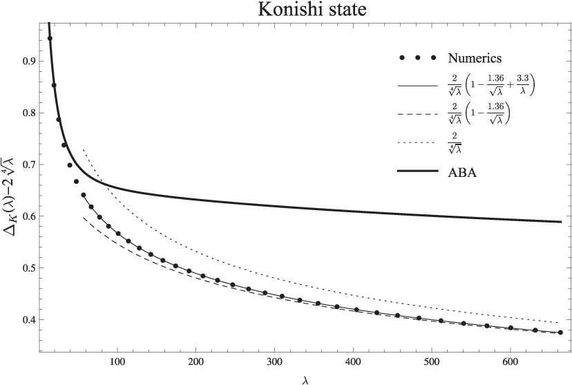
The leading term reproduces indeed the expected large $\lambda$ behavior within our numerical precision. It was also argued in [34] that the subleading coefficient ought to be integer (the next corrections could be transcendental [35]). Indeed, our numerics seems to indicate that $\Delta_{K}=2\lambda^{1/4}+2/\lambda^{1/4}+\dots$ thus predicting the value of this integer!⁴⁴ 4 Assuming the leading coefficient to be $2\lambda^{1/4}$ one gets $1.001$ instead of $0.994$ for the subleading term, even closer to $1$ - the value predicted here. We also obtained predictions for two further subleading corrections (with a lower precision of course).

Our results are represented in Figs.1 and 2.

The Y-system defining the spectrum of all local operators in planar AdS/CFT correspondence reads [14]

$$\frac{Y_{a,s}^{+}Y_{a,s}^{-}}{Y_{a+1,s}Y_{a-1,s}}=\frac{(1+Y_{a,s+1})(1+Y_{a,s-1})}{(1+Y_{a+1,s})(1+Y_{a-1,s})}\,.$$

(2)

where the functions $Y_{a,s}(u)$ correspond only to the nodes marked by ${\includegraphics[scale={0.5}]{ico_b.eps}},{\includegraphics[scale={0.5}]{ico_f1.eps}},{\includegraphics[scale={0.5}]{ico_f2.eps}},{\includegraphics[scale={0.5}]{ico_p.eps}},{\includegraphics[scale={0.5}]{ico_m.eps}}$ on Fig.3 (we will use these notations for $Y$-functions in what follows). The one particle energy at infinite length $\epsilon^{(a)}(u)=a+\frac{2ig}{x^{[-a]}}-\frac{2ig}{x^{[+a]}}$ is defined through the Zhukovski map $x(u)+\frac{1}{x(u)}=\frac{u}{g}\,$ and $f^{[\pm a]}\equiv f(u\pm ia/2),\quad f^{\pm}\equiv f(u\pm i/2)$ for any function $f(u)$. A solution of $Y$-system with a given set of quantum numbers defines the energy of a state (or dimension of an operator in N=4 SYM) through the formula (3) where the Bethe roots $u_{j}$ are fixed by the exact Bethe ansatz equations $Y_{{\includegraphics[scale={0.5}]{ico_m.eps}}_{1}}(u_{j})=-1$.

In this paper we restrict ourselves to the integral form of the $Y$-system for the $SL(2)$-excited states obtained in [15]. Furthermore we focus ourself for simplicity on the Konishi operator where we have only two roots $u_{1}=-u_{2}$ which we can encode into the “Baxter functions" $R^{(\pm)}(u)=(x(u)-x_{1}^{\mp})(x(u)-x_{2}^{\mp})$ and their complex conjugates $B(u)=\bar{R}(u)$ where $x_{1,2}^{\mp}=x(u_{1,2}\mp i/2)$ with the physical choice of branches, such that $|x(u)|>1$, while for the free variable $x(u)$ we should use the mirror kinematics which corresponds to the branches where ${\rm Im}\;(x(u))>0$ [27]. Unless it is explicitly said otherwise, we will be always using this latter choice in what follows. With the mirror choice, $x(u)$ has a semi-infinite cut for $u\in(-\infty,-2g)\cup(2g,+\infty)$. The energy of the Konishi state is computed from

$\displaystyle\Delta_{K}=2+2\epsilon^{(1)}(u_{1})+\sum_{a=1}^{\infty}\int_{-\infty}^{\infty}\frac{du}{2\pi i}\partial_{u}\epsilon^{(a)}\log\left(1+Y_{{\includegraphics[scale={0.5}]{ico_m.eps}}_{a}}\right)\,,$

(3)

where the integral equations defining $Y_{{\includegraphics[scale={0.5}]{ico_m.eps}}_{a}}$ read [15]

	$\displaystyle\log Y_{{\includegraphics[scale={0.5}]{ico_f2.eps}}}\!\!$	$\displaystyle=$	$\displaystyle\!\!K_{m-1}*\log(1+1/Y_{{\includegraphics[scale={0.5}]{ico_b.eps}}_{m}})/(1+Y_{{\includegraphics[scale={0.5}]{ico_p.eps}}_{m}})$
		$\displaystyle+$	$\displaystyle\!\!{\cal R}^{(0m)}*\log(1+Y_{{\includegraphics[scale={0.5}]{ico_m.eps}}_{m}})+\log\frac{-R^{(+)}}{R^{(-)}}$
	$\displaystyle\log Y_{{{\includegraphics[scale={0.5}]{ico_p.eps}}}_{n}}\!\!$	$\displaystyle=$	$\displaystyle\!\!{\cal M}_{nm}*\log(1+Y_{{\includegraphics[scale={0.5}]{ico_m.eps}}_{m}})-K_{n-1}{\circlearrowright\hskip-8.53581pt*\hskip 0.56905pt}\log(1+Y_{{\includegraphics[scale={0.5}]{ico_f2.eps}}})$
		$\displaystyle-$	$\displaystyle\!\!K_{n-1,m-1}*\log(1+Y_{{{\includegraphics[scale={0.5}]{ico_p.eps}}}_{m}})+\log\frac{R_{n}^{(+)}{B_{n-2}^{(+)}}}{R_{n}^{(-)}B_{n-2}^{(-)}}$
	$\displaystyle\log Y_{{{\includegraphics[scale={0.5}]{ico_b.eps}}}_{n}}\!\!$	$\displaystyle=$	$\displaystyle\!\!K_{n\!-\!1,m\!-\!1}\!\!*\!\log(1\!+\!1/Y_{{{\includegraphics[scale={0.5}]{ico_b.eps}}}_{m}}\!)\!+\!K_{n-1}{\circlearrowright\hskip-8.53581pt*\hskip 0.56905pt}\log(1\!+\!Y_{{\includegraphics[scale={0.5}]{ico_f2.eps}}}\!)$
	$\displaystyle\log Y_{{{\includegraphics[scale={0.5}]{ico_m.eps}}}_{n}}\!\!$	$\displaystyle=$	$\displaystyle\!\!{\cal T}_{nm}*\log(1+Y_{{\includegraphics[scale={0.5}]{ico_m.eps}}_{m}})+2{\cal R}^{(n0)}{\circlearrowright\hskip-8.53581pt*\hskip 0.56905pt}\log(1+Y_{{\includegraphics[scale={0.5}]{ico_f2.eps}}})$		(4)
		$\displaystyle+$	$\displaystyle\!\!2{\cal N}_{nm}*\log(1+Y_{{\includegraphics[scale={0.5}]{ico_p.eps}}_{m}})+i\Phi_{n}\,\,.$

We use here the kernels and sources defined in [15] and presented in the appendix for completeness. The integrals in convolutions $K*f=\int dvK(u,v)f(v)$ go along the real axis, but slightly below the poles in the terms involving $Y_{{{\includegraphics[scale={0.5}]{ico_p.eps}}}_{2}}$ (due to the last term in the corresponding integral equation, see [15]). The convolutions ${\circlearrowright\hskip-8.53581pt*\hskip 0.56905pt}$ should be understood in the sense of a B-cycle (see [15]), e.g. ${\cal R}^{(n0)}{\circlearrowright\hskip-8.53581pt*\hskip 0.56905pt}\log(1+Y_{{\includegraphics[scale={0.5}]{ico_f2.eps}}})$ stands for

$$\int_{-2g}^{2g}dv\left[{\cal R}^{(n0)}\log(1+Y_{{\includegraphics[scale={0.5}]{ico_f2.eps}}})-{\cal B}^{(n0)}\log(1+1/Y_{{\includegraphics[scale={0.5}]{ico_f1.eps}}})\right]$$

where $\frac{1}{Y_{{\includegraphics[scale={0.5}]{ico_f1.eps}}}}$ is the analytical continuation of $Y_{{\includegraphics[scale={0.5}]{ico_f2.eps}}}$ across the cut $u\in(-\infty,-2g)\cup(2g,+\infty)$. Summation over the repeated index $m$ is assumed with $m\geq 2$ for ${\includegraphics[scale={0.5}]{ico_p.eps}}_{\pm m}$ and ${\includegraphics[scale={0.5}]{ico_b.eps}}_{\pm m}$, and $m\geq 1$ for ${\includegraphics[scale={0.5}]{ico_m.eps}}_{m}$.

A remarkable feature of all these equations, crucial for the success of our numerics and noticed in [15], is the reality of all $Y$-functions in the integral equations.

The Y-system integral equations for the functions $Y_{a,s}$ need to be supplemented by the exact Bethe equations $Y^{{\rm ph}}_{{{\includegraphics[scale={0.5}]{ico_m.eps}}}_{1}}(u_{j})=-1$ which reproduce the asymptotic Bethe equations of Beisert and Staudacher in the large $L$ limit [14]. To use this equation, we need to analytically continue the last of eq.(4) in the free variable $u$ from mirror to physical plane and then evaluate it at $u=u_{1}$. After some manipulations with contours we find

	$\displaystyle\!\!\!\!\!\log Y^{{\rm ph}}_{{{\includegraphics[scale={0.5}]{ico_m.eps}}}_{1}}(u_{1})\!=\!\tilde{\cal T}_{1m}\!*\!\log(1\!+\!Y_{{\includegraphics[scale={0.5}]{ico_m.eps}}_{m}})\!+\!\log Z_{{\includegraphics[scale={0.5}]{ico_p.eps}}_{2}}\!(u_{1})$		(5)
	$\displaystyle\!\!\!\!\!+i\Phi_{{\rm ph}}(u_{1})+2({\cal R}^{(10)}_{{\rm ph},{\rm mir}}{\circlearrowright\hskip-8.53581pt*\hskip 0.56905pt}K_{m-1}+K_{m-1}^{-})*_{p.v.}\log(Z_{{\includegraphics[scale={0.5}]{ico_p.eps}}_{m}})$
	$\displaystyle\!\!\!\!\!+2{\cal R}^{(10)}_{{\rm ph},{\rm mir}}{\circlearrowright\hskip-8.53581pt*\hskip 0.56905pt}\log(1\!+\!Y_{{\includegraphics[scale={0.5}]{ico_f2.eps}}})\!-\!2\log\tfrac{u_{1}-i/2}{i}\!-\!2\sum_{j=1}^{2}\log\frac{\tfrac{1}{x_{1}^{+}}-x_{j}^{+}}{\tfrac{1}{x_{1}^{-}}-x_{j}^{+}}$

where $*_{p.v.}$. stands for principal value integration, $\tilde{\cal T}_{1m}$ is the dressing phase in the physical kinematics while $i\Phi_{\rm ph}$ is the same as $i\Phi$ but evaluated in the physical region (see appendix). We used $1/Y_{{\includegraphics[scale={0.5}]{ico_f1.eps}}}(u_{j}\pm i/2)=0$ (following from (4)) and denoted $Z_{{\includegraphics[scale={0.5}]{ico_p.eps}}_{m}}=(1+Y_{{\includegraphics[scale={0.5}]{ico_p.eps}}_{m}})(1-1/m^{2})(u^{2}-u_{1}^{2})^{\delta_{m,2}}$ to isolate the poles in $Y_{{\includegraphics[scale={0.5}]{ico_p.eps}}_{2}}$ at $u=u_{j}$ and to ensure decreasing asymptotics at large $u$ which is of course useful for the numerics. Finally, in contrast to $Y^{{\rm ph}}_{{{\includegraphics[scale={0.5}]{ico_m.eps}}}_{1}}(u_{1})$, the term $Z_{{\includegraphics[scale={0.5}]{ico_p.eps}}_{2}}(u_{1})$ is evaluated in mirror kinematics.

We solve the integral equations (4) iteratively for the Konishi state. Namely, we find the $Y$-functions at a step $n$ by plugging the $Y$-functions of step $n-1$ into the r.h.s. of these equations. As the first step of the iterations we use the large $L$, ABA solutions of the $Y$-system [14]. At each step of iterations we also update the position of the Bethe roots by solving the exact Bethe equation of the previous section. It is important to note that the r.h.s. of (5) remains, within our precision, purely imaginary in the process of iterations.

We should also truncate the infinite set of $Y$-functions to some finite number. We explicitly iterate the first $25$ $Y_{{\includegraphics[scale={0.5}]{ico_p.eps}}_{n}}$’s and $25$ $Y_{{\includegraphics[scale={0.5}]{ico_b.eps}}_{n}}$’s at each step. Then we also extrapolate them to obtain extra $40$ $Y_{{\includegraphics[scale={0.5}]{ico_p.eps}}_{n}}$’s and $40$ $Y_{{\includegraphics[scale={0.5}]{ico_b.eps}}_{n}}$’s with higher numbers to replace the infinite sums in (4) on the next step of iteration. For $Y_{{\includegraphics[scale={0.5}]{ico_m.eps}}_{n}}$ we can truncate the sums much earlier (typically $Y_{{\includegraphics[scale={0.5}]{ico_m.eps}}_{2}}/Y_{{\includegraphics[scale={0.5}]{ico_m.eps}}_{1}}\ll 0.1$): the first $5$ of them are largely enough for our precision. Finally, the integrals along the real axis are computed along the stretch $(-X,X)$ with $X$ being a large cut-off. With these approximations, our absolute precision for the energy is around $\pm 0.001$.

We solved the integral equations for a wide range of couplings $0\lesssim\lambda\lesssim 700\gg 1$ stretching from the perturbative region up to this value, which is already a deep strong coupling regime ⁵⁵ 5 The expected world-sheet perturbation theory expansion at strong coupling is $\lambda^{1/4}(a_{1}+a_{2}/\sqrt{\lambda}+\dots)$. The first two coefficients $a_{i}$ - are of order $1$ and we assume that all $a_{i}\sim 1$. In our numerics $1/\sqrt{\lambda}\sim 0.04$. The appropriate extrapolation procedure can easily increase the precision by one order and we expect the absolute numerical error for our $a_{2}$ coefficient to be within $0.005$.. We found no sign of any singularity and the curve looks perfectly smooth. By this reason we believe that any new singularities, such as those related to the Lüscher $\mu$-terms, will not appear. This seems to be the case perturbatively [37] and our numerics seems to indicate that the integral form of Y-system we are solving describes exactly the full spectrum of planar N=4 SYM theory in $SL(2)$ sector. Although we cannot discard a possibility that some new singularities could collide with the integration contours for even larger values of the ’t Hooft coupling (such extra singularities could be easily incorporated into our code), our numerical results suggest that this possibility is very unlikely.

With a precision of $0.001$ we can approximate the Konishi dimension in the range we considered by ${\footnotesize\sqrt[4]{g^{2}+1}}\frac{252.93h^{4}+384.74h^{3}+674.13h^{2}+128.17h+4}{35.67h^{4}+51.43h^{3}+99.71h^{2}+29.29h+1}$ where $h=g^{2}/\sqrt{g^{2}+1}$ and $\lambda=16\pi^{2}g^{2}$ (this function is just a shorthand for the data in Table I).

We presented here a numerical method for solving the Y-system for the Konishi dimension in planar N=4 SYM. It opens the way to the systematic study of the spectrum of many interesting states at any values of the coupling. We also hope to simplify the Y-system in the future using the underlying Hirota integrable dynamics and reducing it to a finite system of integral equations.

We use: ${\cal P}^{(n)}(v)\equiv-\frac{1}{2\pi}\frac{d}{dv}\log\frac{x^{[+n]}_{v}}{x^{[-n]}_{v}}$, $K_{n}\equiv\frac{2n/\pi}{n^{2}+4u^{2}}$ and

	$\displaystyle\!\!\!\!{\cal R}^{(nm)}(u,v)\equiv\frac{\partial_{v}}{2\pi i}\log\frac{x_{u}^{[+n]}-x_{v}^{[-m]}}{x_{u}^{[-n]}-x_{v}^{[+m]}}-\frac{1}{2i}{\cal P}^{(m)}(v)\,,\;\;$
	$\displaystyle\!\!\!\!{\cal B}^{(nm)}(u,v)\equiv\frac{\partial_{v}}{2\pi i}\log\frac{{1/x}_{u}^{[+n]}-x_{v}^{[-m]}}{{1/x}_{u}^{[-n]}-x_{v}^{[+m]}}-\frac{1}{2i}{\cal P}^{(m)}(v)\,,$
	$\displaystyle\!\!\!\!{\cal M}_{nm}\equiv K_{n-1}{\circlearrowright\hskip-8.53581pt*\hskip 0.56905pt}{\cal R}^{(0m)}+K^{\neq}_{n-1,m-1}\,,$
	$\displaystyle\!\!\!\!{\cal N}_{nm}\equiv{\cal R}^{(n0)}{\circlearrowright\hskip-8.53581pt*\hskip 0.56905pt}K_{m-1}+K^{\neq}_{n-1,m-1}\,,$
	$\displaystyle\!\!\!\!K_{nm}\equiv{\cal F}_{n}^{u}\!\circ\!{\cal F}_{m}^{v}\!\circ\!K_{2}(u-v),\,K_{nm}^{\neq}\equiv{\cal F}_{n}^{u}\!\circ\!{\cal F}_{m}^{v}\!\circ\!K_{1}(u-v)\,,$

where the fusion operation ${\cal F}_{n}^{u}\circ A\equiv\sum_{k=-\frac{n-1}{2}}^{\frac{n-1}{2}}A(u+ik)$. Finally, we also use a nice integral representation [15] of the kernel ${\cal T}_{n,m}$ given by

	$\displaystyle\!\!\!\!{\cal T}_{n,m}(u,v)=-{K}_{n,m}(u-v)-\frac{in}{2}\mathcal{P}^{(m)}(v)\,,$		(6)
	$\displaystyle\!\!\!\!-2\sum_{a=1}^{\infty}\int\!\!\left[{\cal B}^{(10)}_{n1}\left(u,w+i\tfrac{a}{2}\right){\cal B}_{1m}^{(01)}\left(w-i\tfrac{a}{2},v\right)+c.c.\right]dw\,\,,$

where ${\cal B}^{(10)}_{nm}={\cal F}_{n}^{u}\circ{\cal F}_{m}^{v}\circ{\cal B}^{(10)}$. For the exact Bethe equations we should use this kernel in the mixed representation,

	$\displaystyle\!\!\!\!\tilde{\cal T}_{1m}=-\sum_{a=1}^{\infty}2{\cal B}_{{\rm ph},{\rm mir}}^{(10)}(u,w+i\tfrac{a}{2})\!*\!{\cal B}_{{\rm mir},{\rm mir}}^{(0m)}(w-i\tfrac{a}{2},v)$
	$\displaystyle\!\!\!\!-\sum_{a=1}^{\infty}2{\cal B}^{(10)}_{{\rm ph},{\rm mir}}(u,w-i\tfrac{a}{2}-i0)\!*\!{\cal B}_{{\rm mir},{\rm mir}}^{(0m)}(w+i\tfrac{a}{2},v)-{K}_{1m}\,.$

Finally the source term $\Phi_{n}(u)={\cal F}_{n}^{u}\circ\Phi(u)$, with

$$\Phi(u)=\frac{1}{i}\log\left[\left(\frac{{x}^{-}}{{x}^{+}}\right)^{L+M}S^{2}\frac{B^{(+)+}R^{(-)-}}{B^{(-)-}R^{(+)+}}\right]\;$$

(7)

where the BES [13] dressing phase $S(u)=\prod_{j=1}^{2}\sigma\left(x^{[\pm]},x_{j}^{\pm}\right)$ should be taken in the mixed, mirror-physical representation in the integral equations and in the physical-physical representation for $\Phi_{\rm ph}$ appearing in the exact Bethe equations. We use the mirror-physical integral representation [15]

	$\displaystyle\log S=\log\frac{B^{(-)+}}{B^{(+)+}}$		(8)
	$\displaystyle+\left({\cal B}^{(10)}(u,w+i0)*{\cal G}*\log\frac{R^{(+)}(u-i0)}{R^{(-)}(u-i0)}+c.c.\right)$

where ${\cal G}(u)\equiv\frac{\partial_{u}}{2\pi i}\log\frac{\Gamma(1-iu)}{\Gamma(1+iu)}$ while for the physical-physical representation we can use the DHM integral representation [38]. Finally ${\mathcal{K}}_{{\rm ph},{\rm mr}}(u,v)$ represents a kernel where we use the physical (mirror) branches for $u$ ($v$). For Konishi $L=2$ and it has $M=2$ derivatives.

Acknowledgments

The work of NG was partly supported by the German Science Foundation (DFG) under the Collaborative Research Center (SFB) 676 and RFFI project grant 06-02-16786. The work of VK was partly supported by the ANR grants INT-AdS/CFT (ANR36ADSCSTZ) and GranMA (BLAN-08-1-313695) and the grant RFFI 08-02-00287. We thank G. Arutyunov, S. Frolov, R. Hernandez, R. Janik, L. Lipatov, T. Lukowski, E. Lopez, A. Rej, R. Roiban, R. Suzuki, M. Staudacher, A. Tseytlin and K. Zarembo for interesting discussions. NG and PV would like to thank CFP for hospitality and computational facilities.

References

- [1] J. M. Maldacena, Adv. Theor. Math. Phys. 2 (1998) 231 [Int. J. Theor. Phys. 38 (1999) 1113]; S. S. Gubser, I. R. Klebanov and A. M. Polyakov, Phys. Lett. B 428 (1998) 105; E. Witten, Adv. Theor. Math. Phys. 2 (1998) 253
- [2] J. A. Minahan and K. Zarembo, JHEP 0303 (2003) 013
- [3] I. Bena, J. Polchinski and R. Roiban, Phys. Rev. D 69 (2004) 046002
- [4] N. Beisert, C. Kristjansen and M. Staudacher, Nucl. Phys. B 664 (2003) 131
- [5] V. A. Kazakov, A. Marshakov, J. A. Minahan and K. Zarembo, JHEP 0405, 024 (2004)
- [6] N. Beisert, V. A. Kazakov, K. Sakai and K. Zarembo, Commun. Math. Phys. 263, 659 (2006)
- [7] R. A. Janik, Phys. Rev. D 73, 086006 (2006)
- [8] M. Staudacher, JHEP 0505, 054 (2005)
- [9] N. Beisert, Adv. Theor. Math. Phys. 12, 945 (2008)
- [10] G. Arutyunov, S. Frolov and M. Staudacher,JHEP 10 (2004) 016.
- [11] N. Beisert, R. Hernandez and E. Lopez, JHEP 0611 (2006) 070
- [12] M. Bianchi, S. Kovacs, G. Rossi and Y. S. Stanev, JHEP 0105 (2001) 042.; B. Eden, C. Jarczak, E. Sokatchev and Y. S. Stanev, Nucl. Phys. B 722, 119 (2005).
- [13] N. Beisert, B. Eden and M. Staudacher, J. Stat. Mech. 0701 (2007) P021
- [14] N. Gromov, V. Kazakov and P. Vieira, arXiv:0901.3753.
- [15] N. Gromov, V. Kazakov, A. Kozak and P. Vieira, arXiv:0902.4458 [hep-th].
- [16] D. Bombardelli, D. Fioravanti and R. Tateo, arXiv:0902.3930 [hep-th].
- [17] G. Arutyunov and S. Frolov, arXiv:0903.0141 [hep-th].
- [18] Al. B. Zamolodchikov, Phys. Lett. B 253 (1991) 391.
- [19] N. Dorey, J. Phys. A 39, 13119 (2006)
- [20] M. Takahashi, Cambridge University Press, 1999.
- [21] F.H.L. Essler, H.Frahm, F.Göhmann, A. Klümper and V. Korepin, Cambridge University Press, 2005.
- [22] V.Bazhanov, S.Lukyanov and A.Zamolodchikov, Nucl. Phys. B 489, 487 (1997)
- [23] P. Dorey and R. Tateo, Nucl. Phys. B 482, 639 (1996)
- [24] D. Fioravanti, A. Mariottini, E. Quattrini and F. Ravanini, Phys. Lett. B 390 (1997) 243
- [25] G. Arutyunov and S. Frolov, JHEP 0903 (2009) 152
- [26] J. Ambjorn, R. A. Janik and C. Kristjansen, Nucl. Phys. B736 (2006) 288–301
- [27] G. Arutyunov and S. Frolov, JHEP 0712 (2007) 024
- [28] S. Frolov and R. Suzuki, arXiv:0906.0499 [hep-th].
- [29] Z. Bajnok and R. A. Janik, Nucl. Phys. B 807, 625 (2009)
- [30] Z. Bajnok, R. A. Janik and T. Lukowski arXiv:0811.4448
- [31] F. Fiamberti, A. Santambrogio, C. Sieg and D. Zanon, Nucl. Phys. B 805 (2008) 231; V. N. Velizhanin, arXiv:0811.0607 [hep-th]
- [32] N. Beisert, T. McLoughlin and R. Roiban, Phys. Rev. D 76 (2007) 046002 [arXiv:0705.0321 [hep-th]].
- [33] S. S. Gubser, I. R. Klebanov and A. M. Polyakov, Nucl. Phys. B 636 (2002) 99
- [34] R.Roiban, A.Tseytlin, arXiv:0906.4294, (see A. Tseytlin’s talk at Shifmania 2009).
- [35] A. Tirziu and A. A. Tseytlin, Phys. Rev. D 78 (2008) 066002
- [36] V. Kazakov, A. Sorin and A. Zabrodin, Nucl. Phys. B 790, 345 (2008)
- [37] Z. Bajnok, A. Hegedus, R. Janik, T. Lukowski, arXiv:0906.4062 [hep-th].
- [38] N. Dorey, D. M. Hofman and J. M. Maldacena, Phys. Rev. D 76 (2007) 025011