Comparing AdS/CFT Calculations to HERA Data
Abstract
We show that HERA data for the inclusive structure function at small Bjorken- and can be reasonably well described by a color-dipole model with an AdS/CFT-inspired dipole-proton cross section. The model contains only three free parameters fitted to data. In our AdS/CFT-based parameterization the saturation scale varies in the range of becoming independent of energy/Bjorken- at very small . This leads to the prediction of -independence of the and structure functions at very small . We provide predictions for and in the kinematic regions of future experiments. We discuss the limitations of our approach and its applicability region, and argue that our AdS/CFT-based model of non-perturbative physics could be viewed as complimentary to the perturbative description of data based on saturation/Color Glass Condensate physics.
pacs
24.85.+p,25.75.-q, 12.38.Mh,13.85.NiAugust 24, 2026
I Introduction
Experimental measurements of the proton structure function in deep inelastic lepton-hadron scattering (DIS) at small Bjorken- have been one of the most valuable sources of information for the exploration of a new regime of QCD which is characterized by high parton density. For sufficiently high energies/small Bjorken-x, perturbative QCD predicts that gluons in a hadron wavefunction form a Color Glass Condensate (CGC) [1, 3, 2, 4]. The main principle of the CGC is the existence of a hard saturation scale at which nonlinear gluons recombination effects start to become important. The saturation scale insures that the strong coupling constant is small.
The saturation scale grows rapidly with energy or a power of as follows from the perturbative nonlinear small-x Balitsky-Kovchegov (BK) [2] and Jalilian-Marian–Iancu–McLerran–Weigert–Leonidov–Kovner (JIMWLK) [3] quantum evolution equations. The BK and JIMWLK evolution equations unitarize the linear Balitsky-Fadin-Kuraev-Lipatov (BFKL) [5] evolution equation at small- in the large- limit (BK) and beyond (JIMWLK). In the leading logarithmic () approximation at fixed coupling, the BK equation predicts that ( is the strong coupling) [6, 7], which is a much faster growth of the saturation scale than one expects phenomenologically from HERA data. On the other hand, it has been shown that next-to-leading-order (NLO) corrections to the BFKL equation (and therefore to BK and JIMWLK kernels) are large and negative [8]: they slow down the growth of the cross sections (and, therefore, of the saturation scale) with energy too much for the theory to fit the data. It is generally believed that the higher order corrections to the NLO BK and JIMWLK equations should remedy this problem and bring CGC theoretical predictions closer to the experimental data. This idea has been recently supported by the phenomenological success of the inclusion of running coupling corrections into the BFKL, BK and JIMWLK equations [9, 10, 11].
Another possible way to constrain higher order corrections to the BFKL, BK and JIMWLK equations is to consider small- evolution in the large coupling limit. At large coupling all higher order perturbative corrections are summed up: thus the behavior of the scattering amplitude and cross sections at strong coupling should serve as a guide to estimate the size of higher order corrections to the perturbative (small coupling) evolution equations. Indeed strong coupling analytic calculations are not possible in QCD. In light of this, one may resort to other QCD-like theories, such as super Yang-Mills (YM) where one can perform calculations in the non-perturbative limit of large ‘t Hooft coupling by employing the Anti-de Sitter space/conformal field theory (AdS/CFT) correspondence [12]. Analysis of high energy scattering amplitudes in the AdS/CFT framework was pioneered in [13, 14]. Applications of AdS/CFT techniques to DIS were further developed in [15].
Very recently, the authors of [17] calculated the total cross-section for a quark dipole scattering on a nucleus at high energy for a strongly coupled super Yang-Mills (SYM) theory using AdS/CFT correspondence. The forward scattering amplitude for the dipole-nucleus scattering was derived in [17] and exhibited an interesting feature: at high energy the amplitude would stop growing with energy, becoming a constant. Such phenomenon happens even for the range of dipole sizes where the interaction is still not very strong, outside of the black disk limit. At very small dipole sizes the amplitude continues to grow fast with energy, in qualitative agreement with the findings of [13, 14] (see [17] for details). The slow growth with energy of the DIS cross section found in [17] may allow one to identify it with the soft pomeron contribution [16]. As such the amplitude may be compatible to DIS data in the (presumably) non-perturbative region of small . Indeed one has to keep in mind that the results of [17] were derived for SYM theory, and their relation to QCD should be qualitative at best.
The main aim of this paper is to confront the color-dipole scattering amplitude on a nucleus from [17] with the available HERA data. It is not a priori obvious whether the available data at HERA are in the kinematics regime of validity of this model. Given the non-perturbative nature of the AdS/CFT approach, we expect this model to be valid at small but also at small where the experimental data is very limited. Below we show that the HERA data for the inclusive structure function for and can be well described within the color dipole picture inspired by the AdS/CFT approach of [17]. We extract the saturation scale from the dipole-proton scattering amplitude fitted to HERA data. We show that, unlike the perturbative predictions for its behavior, the saturation scale given by the AdS/CFT approach of [17] becomes independent of energy/Bjorken-x at very high energy, while being energy-dependent at lower energies. This leads to a new phenomenon, the -independent behavior of structure function at very small and . We point out that qualitatively similar behavior of (i.e., slowing down of the -dependence at small-) is expected from the CGC approach as well [11].
The paper is organized as follows: in Sect. II we briefly recall the color dipole description of structure function . In Sect. III we introduce the AdS/CFT model for the dipole-target forward scattering amplitude. In Sect. IV we present our AdS-inspired fit to the HERA data. In Sect. V we plot our fit for the structure function and extend our curves to make predictions for smaller values of than measured at HERA. We do the same for the charm structure function . We also make predictions for the longitudinal structure function and the total photoproduction cross section. As a conclusion, in Sect. VI we highlight the main results, and discuss the prospects and caveats of our model.
II Color dipole description of structure function
One of the most promising approaches to description of the DIS total and diffractive lepton-proton cross sections at small has been the color dipole factorization scheme. In the color-dipole picture the scattering between the virtual photon and the proton is seen as the dissociation of into quark-antiquark pair (the so-called dipole) of flavor with transverse size which then interacts with the proton via gluon exchanges and emissions,
| (1) |
where the light-cone wavefunction for is computable in QED [18, 19, 20] with denoting the longitudinal and transverse polarizations of the virtual photon:
| (2a) | |||||
| (2b) | |||||
Here is the fraction of the light cone momentum of the virtual photon carried by the quark, is quark mass, , is the electromagnetic coupling constant, is the electric charge of a quark with flavor , and denotes the number of colors. Below, we will first follow [19] and use three light quark flavors only with MeV. Then, we will also consider a case with three light flavors and a charm quark with mass GeV. To estimate the effect of light quark masses, we will also consider a case with massless light quarks. For the light quarks, the gluon density is evaluated at (Bjorken-x), while for charm quarks we take .
The dipole-proton cross-section incorporates QCD effects. It is usually written as an integral of the imaginary part of the forward scattering amplitude over the impact parameter [2]:
| (3) |
where bold letters denote two-dimensional vectors in transverse plane. Following the usual approach we will neglect the -dependence in making the integral in Eq. (3) trivial giving the proton’s transverse area factor: .
The proton structure function and the longitudinal structure function can be written in terms of cross-section,
| (4) | |||||
| (5) |
The contribution of the charm quark to the wave functions in Eqs. (2) feeds into Eqs. (1) and (4) directly giving the charm structure function . In the CGC framework the dipole-proton forward scattering amplitude can be found by solving BK or JIMWLK evolution equations [21, 11]. Alternatively there exist many different phenomenological approaches to model both CGC and non-perturbative effects in the dipole cross-section or amplitude which can be then tested against the HERA data, see [22] and references therein. Here, we show that the AdS/CFT-inspired color-dipole model of [17] predicts a new scaling behavior for the proton structure function at very small and in a region where there is no experimental data yet and argue that future experimental measurement of in this region can be used to test the model.
III AdS/CFT color dipole model
The forward scattering amplitude of a dipole on a large nuclear target (with atomic number ) at high-energy for a strongly coupled super Yang-Mills theory employing AdS/CFT correspondence was derived in [17] and has the following form:
| (6) | |||||
| (7) | |||||
| (8) | |||||
| (9) |
The parameter in the above equations is a constant which relates the transverse dipole size , the collision energy and the maximum extent of the string in the -direction labeled by [17],
| (10) |
where the value of is given by11 1 From Eq. (10) one can immediately recover the case considered by Maldacena [23] for the shape of a static Wilson loop in an empty AdS5 space by putting .
| (11) |
The parameter in Eq. (6) is given by
| (12) |
where denotes the ‘t Hooft coupling with the Yang-Mills coupling constant. The parameter can be identified as the transverse momentum scale [17]. Note that in Eq. (8) can be imaginary for small , but the parameter is always real.
One can also rewrite the dipole amplitude Eq. (6) as a function of Bjorken-. To simplify and approximate the -integral in Eq. (1) we relate the virtuality of the photon to the dipole size where the parameter will be determined from a fit to the data. Therefore, the Bjorken- variable in DIS becomes22 2 Note that we ignore the proton mass in the Bjorken-x definition since its effects in the kinematic region of our interest is negligible and will not change the results.
| (13) |
By using the above relation, one can rewrite the dipole-nucleus amplitude defined in Eq. (6) as a function of and ,
| (14) |
with
| (15) |
where we defined and . The impact-parameter integrated dipole cross-section on a proton target is then related to the dipole amplitude via .
As a comparison to other dipole models, we will cross-check our results with the popular GBW color dipole model proposed by Golec-Biernat and Wüsthoff [19]. This model is able to describe DIS data with the dipole cross-section parametrized as
| (16) |
where -dependence of the saturation scale is given by
| (17) |
We have not assumed anything about the functional form of the saturation scale in the dipole amplitude (14). Note that there is no unique definition for the saturation scale in literature. Following Refs. [19, 24, 25, 26] we define a saturation scale as a momentum scale at which the dipole scattering amplitude becomes sizable
| (18) |
For the GBW model, this definition coincides with the saturation scale defined in Eq. (17). Similarly, the saturation scale in AdS/CFT dipole model (14) is then defined as
| (19) |
Note that the AdS/CFT dipole scattering amplitude from Eq. (14) with the saturation scale from Eq. (19) exhibits the property of geometric scaling [27]: it is a function of only, . Moreover, the anomalous dimension in the AdS/CFT dipole model is which is rather close to the value of obtained from the numerical solution of the BK equation [28]. Thus in many ways our AdS/CFT inspired model is similar to the predictions of CGC. The main difference is in the -dependence of the saturation scale , which we will discuss shortly.
IV Fit to HERA Data
In this section, we confront the AdS/CFT color-dipole with the experimental data from DIS and test its validity by investigating whether its free parameters can be fitted to the experimental measurements of the proton structure function .
In the dipole amplitude given by Eqs. (14) we take to be a free parameter since the value of is not known. The parameters and always appear only as a product denoted by and cannot be taken in the fitting as two independent parameters. By taking as a free parameter, we also allow the parameter to deviate from its value obtained from the AdS/CFT approach. This is motivated by the fact that the value of given by Eq. (11) is true for SYM theory, and is likely to be different for QCD. The parameter in the AdS/CFT dipole model appears as an overall factor in the saturation scale in Eq. (19): it can be taken as another free parameter in the fit. As and only appear together in we put GeV throughout this paper and vary . We examine different cases with and . The other two free parameters and in the AdS/CFT dipole model will be determined from a fit to the DIS data. Notice that the GBW dipole model given by Eq. (16) also has unknown parameters: , and .
| AdS/CFT dipole model | ||||
|---|---|---|---|---|
| GBW dipole model | ||||
|---|---|---|---|---|
We shall use HERA data from ZEUS [30, 31, 32, 33] measurement of . Following the earlier analysis Refs. [24, 25, 26, 29, 34], we do not include the H1 data in order to avoid introducing extra normalization parameters relating ZEUS and H1 data. The AdS/CFT color dipole model is motivated by non-perturbative QCD and could only be applicable at small . Therefore, we are interested in small and where most data is from ZEUS. Unfortunately the experimental data points for the structure function at very small and are very limited.
Note that the GBW model is motivated by the perturbative QCD and its validity at very small is questionable, though it can be extended to higher if the full DGLAP evolution is used. For the same reason, in the earlier analysis of the GBW model, the data below was not included in the fitting [19], although inclusion of those data does not have a significant effect on the parameters obtained from the fit (see also table II). Here, we use the GBW model only as a benchmark in order to compare our results with a perturbatively motivated dipole model.
| 140 | |||||
| 0 |
The resulting parameters of the AdS/CFT and the GBW color-dipole models and values obtained from the fit in which we consider only three light flavors with the quark mass are presented in tables I and II for the same data bin. From table II, it is seen that the parameters of the GBW model obtained from the fit to the data bin of are very similar to those in the case when one takes all the data within [25]. However, the value of the intercept increases from to when we limit the data to a lower virtuality . The value of is consistent with perturbative predictions based on small- evolution with running coupling and other higher order corrections [35, 11, 9, 6, 36]. The quality of the fit based on the AdS/CFT color-dipole model is very sensitive to the upper bound of the given Bjorken- bin. This can be seen in table I where including data with dramatically increases and worsens the fit. This is in contrast to the GBW model which gives a surprisingly good fit for a wide range of (see also table II). We show in table I that a good fit with (with ) for the AdS/CFT dipole amplitude can be found for the current available data within and . Note that currently there is no experimental data below the lower and bound we have taken, and also there is no experimental data for at large but very small . In table I, we also show the results of the fit to the same data bin for different values of . Notice that our model is valid in the non-perturbative regime, therefore we do not expect a very small value of . However, with a smaller we can relax the upper bound on the -bin and find a good fit for even larger . It is also seen from table I that for a wide range of , the results of the fit change only little.
While the smaller values of appear to give better description of the data using our AdS/CFT ansatz, one has to keep in mind that AdS/CFT correspondence is valid for . We therefore can not use very small in the fit, as the whole underlying theoretical approach of [17] would reach its limit of applicability. At smaller higher order string excitations become important introducing corrections to the single-pomeron intercept [14] and probably to the rest of the expression (6). To (roughly) quantify how small the coupling can be with our ansatz (6) still remaining dominant we notice that string excitations corrections calculated in the second reference in [14] modify the pomeron intercept in the amplitude from to . For the correction to be small one needs . In our analysis here we therefore restrict to be . Indeed in QCD at low- one has , which is in the range of considered in our fits. Values of for QCD as low as in AdS/CFT framework have been considered in the literature [37] to describe RHIC heavy ion data.
In table III, we present our fits for the AdS/CFT dipole model in the presence of charm quark. It can be seen that while the inclusion of charm quark slightly worsens the fit, nevertheless is still in the acceptable range. In tables III, IV to investigate the importance of the value of light quark masses, we also show the results of the fit (to two different data bins for the two tables) in which the light quark masses are taken to be zero, . For comparison, we also show the results of the fit obtained with MeV for the same data bins. It can be seen that taking improves the fit somewhat. One has to keep in mind that the AdS/CFT dipole amplitude (6) was calculated in [17] for very heavy dressed (constituent) quarks: extrapolating it to massless quarks pushes Eq. (6) closer to the theoretical limit of its applicability. In practice, due to the largeness of the saturation scale in this model (see below), the structure function is not very sensitive to light quark masses in the range of that we consider. One may expect that, since the AdS/CFT calculation of [17] was done for heavy quarks, the fit should improve with the inclusion of charm. However, note that large charm quark mass makes QCD coupling small making corresponding QCD physics more perturbative. As the AdS/CFT calculation we are using is valid for large coupling only, inclusion of charm also pushes the model to the limit of its applicability. This could be the reason the fit gets slightly worse when we include charm quark mass. Another potential danger of including heavy flavor is in the fact that they shorten the typical coherence length of the quark dipole, potentially making it smaller than the size of the proton and invalidating the dipole approach altogether. This is a problem common to all dipole models.
The value of obtained from the fit (in tables I, III and IV) is surprisingly small. The parameter relates the virtuality of the photon to the dipole size, and one expects it to be of order of one. On the other hand, the parameter obtained from the AdS/CFT approach Eq. (11) is in SYM theory. In order to clarify whether the smallness of should be associated with or with we employed -dependent AdS/CFT dipole model defined in Eqs. (6-9) which has the parameter but no . (That is we undid the numerical simplification we had made by writing to define Bjorken in Eq. (13).) We first tried to keep the parameter fixed as given in the AdS/CFT approach. However, this did not lead to a good fit for a wide range of . Then, arguing that should be different in QCD as compared to in SYM theory, we considered the parameter to be a free parameter and determined it from the fit. In table V, we show the results of the fit for different fixed values of . It is seen that generally the preferred value of from the fit is two orders of magnitude smaller than the AdS/CFT value. This is consistent with the smallness of obtained from the -dependent AdS/CFT dipole model. Therefore, the smallness of is due to the smallness of the parameter preferred by HERA data.


V Plots and predictions
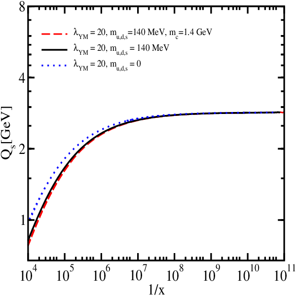
Let us now plot the structure function given by our fit presented above. In Fig. 1, we show the description of the proton structure function obtained from the fit given in table I for the AdS/CFT and in table II for the GBW dipole model. Notice that although both models give a good fit of existing data, they lead to drastically different predictions for the structure function at smaller in the region where there is no experimental data yet. The main prediction of the AdS/CFT color-dipole model is that at very small it gives rise to a saturating behavior of the structure function which becomes independent of . The onset of this limiting (scaling) behavior moves to a smaller for larger . This can be also seen from Fig. 2 where in the left panel we plot the AdS/CFT dipole cross-section as a function of the dipole transverse size . It is obvious that AdS/CFT dipole cross-section profile saturates for and will not change further with . This is in contrast with the GBW model (and other available dipole models) where the dipole cross-section rapidly changes as we move toward smaller , though a certain slowing down of the -dependence at small- is observed in [11] due to running coupling effects. In the right panel of Fig. 2 we show the saturation scale for both the AdS/CFT and the GBW dipole models. It can be seen that the saturation scale in AdS/CFT dipole model is smaller than the one obtained from the GBW model at very small . Moreover, the AdS/CFT model of [17] predicts that the saturation scale saturates. The saturation scale in the AdS/CFT dipole model defined via Eq. (19) is proportional to . Therefore, smaller leads to a smaller saturation scale. One can also see from Fig. 3 that the saturation scales for the case of massless light flavors only () and also for the case of massive light quarks with MeV with the charm quark included are very similar to the case of three light flavors only with MeV. This independence of the saturation scale of the light quark masses is due to the large saturation scale in this model, which cuts off the infrared effects making the physics less sensitive to the quark masses. The fact that the saturation scale in Fig. 3 is rather large probably explains why the charm quark mass does not affect it either. The curves for the structure function in the massless light quarks case are not very different visually from the massive quarks case curves shown in Fig. 1 already: that is why we do not show the massless case curves there.


In Fig. 4, we plot the charm structure function given by our AdS/CFT dipole model. Note that we use a fit to data (table III) within the range of and . Therefore the experimental data in Fig. 4 are beyond the range of our fit. Moreover, the large values of in Fig. 4 push our AdS-inspired model to the limit of its validity. Hence the curves in Fig. 4 can be thought of as predictions of our model. We see that the agreement with data even in this region is rather good.
In Fig. 5, we show the predictions of our AdS-inspired model for the longitudinal structure function calculated using Eq. (5). We use the same fits as employed in Fig. 1. Unfortunately currently there is no data for at low and low where our model is valid. It can be seen from Fig. 5 that a precise measurement of at small and can offer a complimentary information which may help one discriminate between different DIS models.


In Fig. 6, we show our predictions for the total photoproduction cross section . It is calculated by taking at . (As can be seen from Eqs. (1) and (2b), at and does not need to be included.) One can see that using the same effective quark mass MeV as in the fit our model slightly overestimates photoproduction data, though mostly remains withing the error bars of the data points. To show the effect of light quark mass on photoproduction cross section we also show the predictions of our model for MeV, which go directly through the photoproduction data. Indeed using MeV would lead to larger of the fit presented above. Therefore, the real predictions of our model are for MeV and slightly miss photoproduction data. (We checked that including charm quark will not improve the fit either.) There could be several reasons for this small discrepancy, one of them being that, after all, the AdS/CFT calculation [17] was not done for QCD, but for a different theory, SYM. For photoproduction the most important difference between QCD and SYM theory is probably the absence of confinement in the latter. As one can see from Eqs. (1) and (2a), the integrand of Eq. (1) falls off as for and decays exponentially () for . (The exponential falloff is due to the light-cone wavefunction (2a) which contains the modified Bessel function which decays exponentially at large values of the argument.) Exponential decay is essential for convergence of the integral over in Eq. (1). We see that the effective infrared cutoff of the -integral is and the resulting cross section depends logarithmically on . In case of photoproduction (for ) we have . Therefore the non-perturbative light quark mass serves as the only infrared cutoff of the -integral in Eq. (1) in the photoproduction () limit, as the photoproduction cross section becomes infinite for . Hence in QCD photoproduction cross section is dominated by non-perturbative effects: this is the basis for the vector meson dominance models. While AdS/CFT calculation [17] does indeed contain non-perturbative effects, it is done for a theory without confinement, allowing for the slight disagreement between our MeV curves and the data in Fig. 6.


Note that we have not included total photoproduction cross-section data in obtaining the fit given in table V since there are only few data points at high energies with rather large error bars. The lower-energy photoproduction data points, while exist [39], are beyond the limit of applicability of our high-energy model. It has been already shown that it is very difficult to simultaneously describe the low energy photoproduction total cross-section and data with a single color dipole amplitude without any extra input [41]. This is partly due to the fact that the color dipole approach is not valid at low energy as the coherence length becomes too short compared to the size of the target proton. One should also bear in mind that the AdS/CFT color dipole amplitude was derived while modeling the proton by an ultra-relativistic shock wave, which may not be a good approximation for lower energy scattering.
From Figs. 1, 4, 5 and 6 it is again clear that the AdS/CFT color dipole model predicts that at low virtuality and at very high energy/very small-, the underlying dipole-target cross section should become independent of or , leading to a plateau in the -dependence for , , and the total photoproduction cross-section.
VI Discussion
In this paper we have demonstrated that the AdS/CFT-inspired parameterization of the dipole amplitude is consistent with the existing low- HERA data for the structure function. The AdS/CFT parameterization of the dipole amplitude allows to make distinct predictions for and structure functions at values of below those where the data exist. In particular our AdS/CFT-inspired model predicts -independence of the structure functions and at very small-. Hence the predictions of our AdS/CFT parameterization can be tested at the future colliders, such as LHC and the proposed LHeC.
Indeed to make the above AdS/CFT model fit the data we had to assume that is about two orders of magnitude smaller than predicted by classical AdS/CFT calculations of [17]. The discrepancy between the two results may be due to the difference between SYM theory and QCD. One should also remember that the calculation of [17] was purely classical (extremizing the string profile in the classical gravity background), and quantum corrections of the order of may be important for the description of the data. Further research is needed to quantify these issues.
A more general question about the applicability of strong-coupling based methods like AdS/CFT to the description of DIS data also has to be asked. Indeed if the strong coupling constant always runs with , then at low- considered above the coupling should be large justifying the use of non-perturbative approaches. At the same time at low- but with small enough for to be large, it is likely that the coupling runs with the saturation scale . As the proton’s saturation scale for the range of small considered above varies in the interval of GeV for most models [19, 9, 11], one could then argue that the problem is perturbative and strongly-coupled methods are not needed to describe the DIS data. Indeed purely perturbative CGC approaches are rather successful in describing the DIS data (see [11] for the most comprehensive and rigorous CGC calculation to date). However, it is likely that the story is more complicated: as one can see in the explicit running coupling calculations [10] for the BK and JIMWLK equations, the strong coupling runs with the size of the dipoles, which indeed varies from non-perturbative to perturbative distance scales. Hence even at large the non-perturbative contribution to may be non-negligible, though it does tend to be suppressed as grows very large. Our work above could be viewed as an effort to estimate the shape of the contribution of the non-perturbative physics to the structure function. We find it rather interesting that, modulo the above-mentioned open questions, the non-perturbative AdS/CFT-inspired physics can be made largely consistent with the data at small-.
Acknowledgements.
Yu.K. would like to thank Boris Kopeliovich, Irina Potashnikova, and the Theoretical Physics group at the Universidad Técnica Federico Santa María in Valparaíso, Chile for their hospitality and support during the initial stages of this work. Yu.K. is also grateful to Genya Levin for informative discussions. The work of Yu.K. is sponsored in part by the U.S. Department of Energy under Grant No. DE-FG02-05ER41377. The work of Z.L. is supported by PBCT (Chile) project ACT-028. A.H.R. would like to thank Boris Kopeliovich for useful discussions. A.H.R. is very grateful to the hospitality of Andreas Schäfer group at Universität Regensburg where this work was finalized, and acknowledges the financial support from Conicyt Programa Bicentenario PSD-91-2006, Fondecyt grants 1090312 (Chile) and the Alexander von Humboldt foundation (Germany). The authors are grateful to Javier Albacete for a useful suggestion.References
- [1] L. V. Gribov, E. M. Levin, and M. G. Ryskin, Phys. Rept. 100 (1983) 1; A. H. Mueller and J.-w. Qiu, Nucl. Phys. B268 (1986) 427; L. D. McLerran and R. Venugopalan, Phys. Rev. D50 (1994) 2225; L. D. McLerran and R. Venugopalan, Phys. Rev. D49 (1994) 3352; L. D. McLerran and R. Venugopalan, Phys. Rev. D49 (1994) 2233; Y. V. Kovchegov, Phys. Rev. D54 (1996) 5463; Y. V. Kovchegov, Phys. Rev. D55 (1997) 5445; J. Jalilian-Marian, A. Kovner, L. D. McLerran, and H. Weigert, Phys. Rev. D55 (1997) 5414.
- [2] Y. V. Kovchegov, Phys. Rev. D60 (1999) 034008; Y. V. Kovchegov, Phys. Rev. D61 (2000) 074018; I. Balitsky, Nucl. Phys. B463 (1996) 99; I. Balitsky, hep-ph/9706411; I. Balitsky, Phys. Rev. D60 (1999) 014020.
- [3] J. Jalilian-Marian, A. Kovner, A. Leonidov, and H. Weigert, Nucl. Phys. B504 (1997) 415; J. Jalilian-Marian, A. Kovner, A. Leonidov, and H. Weigert, Phys. Rev. D59 (1998) 014014; J. Jalilian-Marian, A. Kovner, and H. Weigert, Phys. Rev. D59 (1998) 014015; J. Jalilian-Marian, A. Kovner, A. Leonidov, and H. Weigert, Phys. Rev. D59 (1999) 034007; A. Kovner, J. G. Milhano, and H. Weigert, Phys. Rev. D62 (2000) 114005; H. Weigert, Nucl. Phys. A703 (2002) 823; E. Iancu, A. Leonidov, and L. D. McLerran, Nucl. Phys. A692 (2001) 583; E. Ferreiro, E. Iancu, A. Leonidov, and L. McLerran, Nucl. Phys. A703 (2002) 489.
- [4] E. Iancu and R. Venugopalan, hep-ph/0303204; H. Weigert, Prog. Part. Nucl. Phys. 55 (2005) 461; J. Jalilian-Marian and Y. V. Kovchegov, Prog. Part. Nucl. Phys. 56 (2006) 104.
- [5] E. A. Kuraev, L. N. Lipatov, and V. S. Fadin, Sov. Phys. JETP 45 (1977) 199; Y. Y. Balitsky and L. N. Lipatov Sov. J. Nucl. Phys. 28 (1978) 822.
- [6] E. Iancu, K. Itakura, and L. McLerran, Nucl. Phys. A708 (2002) 327.
- [7] J. L. Albacete, N. Armesto, J. G. Milhano, C. A. Salgado, and U. A. Wiedemann, Phys. Rev. D71 (2005) 014003.
- [8] V. S. Fadin and L. N. Lipatov, Phys. Lett. B429 (1998) 127; M. Ciafaloni and G. Camici, Phys. Lett. B430 (1998) 349; I. Balitsky and G. A. Chirilli, Phys. Rev. D77 (2008) 014019; D. A. Ross, Phys. Lett. B431 (1998) 161; Y. V. Kovchegov and A. H. Mueller, Phys. Lett. B439 (1998) 428.
- [9] J. L. Albacete, Phys. Rev. Lett. 99 (2007) 262301; M. Ciafaloni and G. Camici, Phys. Lett. B430 (1998) 349; I. Balitsky and G. A. Chirilli, Phys. Rev. D77 (2008) 014019; D. A. Ross, Phys. Lett. B431 (1998) 161; Y. V. Kovchegov and A. H. Mueller, Phys. Lett. B439 (1998) 428; M. Ciafaloni, D. Colferai, and G. P. Salam, Phys. Rev. D60 (1999) 114036.
- [10] I. I. Balitsky, Phys. Rev. D 75 (2007) 014001; Y. Kovchegov and H. Weigert, Nucl. Phys. A 784 (2007) 188; E. Gardi, J. Kuokkanen, K. Rummukainen, and H. Weigert, Nucl. Phys. A784 (2007) 282; J. L. Albacete and Y. V. Kovchegov, Phys. Rev. D75 (2007) 125021.
- [11] J. L. Albacete, N. Armesto, J. G. Milhano and C. A. Salgado, arXiv:0902.1112.
- [12] J. M. Maldacena, Adv. Theor. Math. Phys. 2 (1998) 231; S. S. Gubser, I. R. Klebanov, and A. M. Polyakov, Phys. Lett. B428 (1998) 105; E. Witten, Adv. Theor. Math. Phys. 2 (1998) 253; O. Aharony, S. S. Gubser, J. M. Maldacena, H. Ooguri, and Y. Oz, Phys. Rept. 323 (2000) 183.
- [13] R. A. Janik and R. B. Peschanski, Nucl. Phys. B 565, 193 (2000) [arXiv:hep-th/9907177].
- [14] J. Polchinski and M. J. Strassler, Phys. Rev. Lett. 88, 031601 (2002) [arXiv:hep-th/0109174]; R. C. Brower, J. Polchinski, M. J. Strassler and C. I. Tan, JHEP 0712, 005 (2007) [arXiv:hep-th/0603115].
- [15] Y. Hatta, E. Iancu and A. H. Mueller, JHEP 0801, 063 (2008) [arXiv:0710.5297]; L. Cornalba and M. S. Costa, Phys. Rev. D 78, 096010 (2008) [arXiv:0804.1562]; P. G. O. Freund and H. Nastase, arXiv:0809.1277; E. Levin, J. Miller, B. Z. Kopeliovich and I. Schmidt, JHEP 0902, 048 (2009) [arXiv:0811.3586].
- [16] A. Donnachie and P. V. Landshoff, Phys. Lett. B 437, 408 (1998) [arXiv:hep-ph/9806344].
- [17] J. L. Albacete, Y. V. Kovchegov and A. Taliotis, JHEP 0807 (2008) 074.
- [18] N. N. Nikolaev and B. G. Zakharov, Z. Phys. C 49, 607 (1991).
- [19] K. Golec-Biernat and M. Wüsthoff, Phys. Rev. D59 (1999) 014017; D60 (1999) 114023.
- [20] Y. V. Kovchegov and L. D. McLerran, Phys. Rev. D 60, 054025 (1999) [Erratum-ibid. D 62, 019901 (2000)] [arXiv:hep-ph/9903246].
- [21] M. Lublinsky, E. Gotsman, E. Levin and U. Maor, Nucl. Phys. A 696, 851 (2001) [arXiv:hep-ph/0102321]; E. Levin and M. Lublinsky, Nucl. Phys. A 696, 833 (2001) [arXiv:hep-ph/0104108].
- [22] L. Motyka, K. Golec-Biernat and G. Watt, arXiv:0809.4191; B. Z. Kopeliovich, A. H. Rezaeian, arXiv:0811.2024; B. Z. Kopeliovich, E. Levin, A. H. Rezaeian and I. Schmidt, Phys. Lett. B675 (2009) 190 [arXiv:0902.4287].
- [23] J. M. Maldacena, Phys. Rev. Lett. 80, 4859 (1998) [arXiv:hep-th/9803002].
- [24] G. Watt and H. Kowalski, Phys. Rev. D78 (2008) 014016.
- [25] H. Kowalski, L. Motyka and G. Watt, Phys. Rev. D74 (2006) 074016.
- [26] H. Kowalski and D. Teaney, Phys. Rev. D68 (2003) 114005.
- [27] A. M. Stasto, K. J. Golec-Biernat and J. Kwiecinski, Phys. Rev. Lett. 86 (2001) 596 [arXiv:hep-ph/0007192].
- [28] D. Boer, A. Utermann and E. Wessels, Phys. Rev. D75 (2007) 094022.
- [29] E. Iancu, K. Itakura and S. Munier, Phys. Lett. B590 (2004) 199.
- [30] J. Breitweg et al. [ZEUS Collaboration], Eur. Phys. J. C7 (1999) 609 [arXiv:hep-ex/9809005].
- [31] M. Derrick et al. [ZEUS Collaboration], Z. Phys. C69 (1996) 607 [arXiv:hep-ex/9510009].
- [32] S. Chekanov et al. [ZEUS Collaboration], Eur. Phys. J. C21 (2001) 443 [arXiv:hep-ex/0105090].
- [33] J. Breitweg et al. [ZEUS Collaboration], Phys. Lett. B487 (2000) 53 [arXiv:hep-ex/0005018].
- [34] J. R. Forshaw and G. Shaw, JHEP 0412 (2004) 052.
- [35] D. N. Triantafyllopoulos, Nucl. Phys. B648 (2003) 293.
- [36] A. H. Mueller and D.N. Triantafyllopoulos, Nucl. Phys. B640 (2002) 331 ; D. N. Triantafyllopoulos, Nucl. Phys. B648 (2003) 293.
- [37] S. S. Gubser, Phys. Rev. D76 (2007) 126003 [arXiv:hep-th/0611272].
- [38] ZEUS Collaboration, Phys. Rev. D69 (2004) 012004.
- [39] H1-collaboration, Phys. Lett. B299 (1993) 374; Z. Phys. C69 (1995) 27.
- [40] ZEUS Collaboration, Nucl. Phys. B627 (2002) 3.
- [41] J. R. Forshaw, G. Kerley and G. Shaw, Phys. Rev. D60 (1999) 074012.