Oscillons in dilaton-scalar theories

Preprint: …

Zalán Horváth Affiliation: Institute for Theoretical Physics, Eötvös University, Márk Mezei Affiliation: H-1117 Budapest, Pázmány Péter sétány 1/A, Hungary

Abstract:

It is shown by both analytical methods and numerical simulations that extremely long living spherically symmetric oscillons appear in virtually any real scalar field theory coupled to a massless dilaton (DS theories). In fact such ”dilatonic” oscillons are already present in the simplest non-trivial DS theory – a free massive scalar field coupled to the dilaton. It is shown that in analogy to the previously considered cases with a single nonlinear scalar field, in DS theories there are also time periodic quasibreathers (QB) associated to small amplitude oscillons. Exploiting the QB picture the radiation law of the small amplitude dilatonic oscillons is determined analytically.

Keywords:

Nonperturbative Effects, Solitons Monopoles and Instantons

1 Introduction

Long-living, spatially localized classical solutions in field theories containing scalar fields exhibiting nearly periodic oscillations in time – oscillons – [1]–[16] have attracted considerable interest in the last few years. Oscillons closely resemble ”true” breathers of the one-dimensional ( $D=1$ ) sine-Gordon (SG) theory, which are time periodic and are exponentially localized in space, but unlike true breathers they are continuously losing energy by radiating slowly. On the other hand oscillons exist for different scalar potentials in various spatial dimensions, in particular for $D=1,2,3$ . Just like a breather, an oscillon possesses a spatially well localized “core”, but it also has a “radiative” region outside of the core. Oscillons appear from rather generic initial data in the course of time evolution in an impressive number of physically relevant theories including the bosonic sector of the standard model [17]–[20]. Moreover they form in physical processes making them of considerable importance [21]–[28]. In a series of papers, [12], [29]–[31], it has been shown that oscillons can be well described by a special class of exactly time-periodic ”quasibreathers” (QB). QBs also possess a well localized core in space (just like true breathers) but in addition they have a standing wave tail whose amplitude is minimized. At this point it is important to emphasize that there are (infinitely) many time periodic solutions characterized by an asymptotically standing wave part. In order to select one solution, we impose the condition that the standing wave amplitude be minimal. This is a physically motivated condition, which heuristically should single out ”the” solution approximating a true breather as well as possible, for which this amplitude is identically zero. The amplitude of the standing wave tail of a QB is closely related to that of the oscillon radiation, therefore its computation is of prime interest. It is a rather non-trivial problem to compute this amplitude even in one spatial dimensional scalar theories [32], [30]. In the limit when the core amplitude is small, we have developed a method to compute the leading part of the exponentially suppressed tail amplitude for a general class of theories in various dimensions [31].

In this paper we show that oscillons also appear in rather general (real) scalar field theories coupled to a (massless) dilaton field (DS theory). Dilaton fields appear naturally in low energy effective field theories derived from superstring models [33, 34, 35] and the study of their effects is of major interest. As the present study shows, the coupling of a dilaton even to a free massive scalar field, referred to as the dilaton-Klein-Gordon (DKG) theory, which is the conceivably simplest non-trivial DS theory, has some rather remarkable consequences. This simple DKG theory already admits QBs and as our numerical investigations show from generic initial data small amplitude oscillons evolve. We concentrate on solutions with the simplest spatial geometry - spherical symmetry. We do not think that considering spherically symmetric configurations is a major restriction since non-symmetric configurations are expected to contain more energy and to evolve into symmetric ones [25]. The dilatonic oscillons are very robust and once formed from the initial data they do not even seem to radiate their energy, hence their lifetime is extremely long (not even detectable by our numerical methods).

Our means for constructing dilatonic oscillons will be the small amplitude expansion, in which the small parameter, $\varepsilon$ , determines the difference of oscillation frequency from the mass threshold. The small amplitude oscillons of the DKG theory appear to be stable in dimensions $D=3,4$ , unstable in $D=5,6$ , and their core amplitude is proportional to $\varepsilon^{2}$ . This is to be contrasted to self-interacting scalar theories whose oscillons are stable in $D=1,2$ , unstable in $D=3$ , and their core amplitude is proportional to $\varepsilon$ . The master equations determining oscillons to leading order in the small amplitude expansion turn out to be the Schrödinger-Newton (SN) equations. The main analytical result of this paper is the analytic computation of the amplitude of the standing wave tail of the dilatonic QBs for any dimension $D$ , and thereby the determination of the radiation law and the lifetime of small amplitude oscillons in DS theories. The used methods have been developed in Refs. [32], [36], [37], [30] and [31].

The above results, namely the stability properties and the SN equations playing the rôle of master equation, show striking similarity to those obtained in the Einstein-Klein-Gordon (EKG) theory, i.e. for a free massive scalar field coupled to Einstein’s gravity, where also stable, long living oscillons (known under the name of oscillating soliton stars, or more recently oscillatons) have been found and investigated in many papers [38]–[44].

2 The scalar-dilaton system

The action of a scalar-dilaton system is

A=\int dt\,d^{D}\!x\left[\frac{1}{2}(\partial_{\mu}\varphi)^{2}+\frac{1}{2}(\partial_{\mu}\Phi)^{2}-e^{-2\kappa\varphi}\,U(\Phi)\right]\,,

(1)

where $\varphi$ is the dilaton field and $\Phi$ is a scalar field with self interaction potential $U(\Phi)$ .

The energy corresponding to the action (1) can be written as

E=\int d^{D}x\,{\cal E}\,,\qquad{\cal{E}}=\frac{1}{2}\left[\left(\partial_{t}\Phi\right)^{2}+\left(\partial_{i}\Phi\right)^{2}+\left(\partial_{t}\varphi\right)^{2}+\left(\partial_{i}\varphi\right)^{2}\right]+e^{-2\kappa\varphi}U(\Phi)\,,

(2)

where ${\cal{E}}$ denotes the energy density. In the case of spherical symmetry

E=\int_{0}^{\infty}dr\,\frac{\pi^{D/2}r^{D-1}}{\Gamma(D/2)}\left[\left(\partial_{t}\Phi\right)^{2}+\left(\partial_{r}\Phi\right)^{2}+\left(\partial_{t}\varphi\right)^{2}+\left(\partial_{r}\varphi\right)^{2}+2e^{-2\kappa\varphi}U(\Phi)\right]\,.

(3)

We assume that the potential can be expanded around its minimum at $\Phi=0$ as

U(\Phi)=\sum_{k=1}^{\infty}\frac{g_{k}}{k+1}\Phi^{k+1}\,,\qquad U^{\prime}(\Phi)=\sum_{k=1}^{\infty}g_{k}\Phi^{k}\ ,

(4)

where $g_{k}$ are real constants. For a free massive scalar field with mass $m$ the only nonzero coefficient is $g_{1}=m^{2}$ . If $g_{2k}=0$ for integer $k$ the potential is symmetric around its minimum. In that case, as we will see, for periodic configurations the Fourier expansion of $\Phi$ in $t$ will contain only odd, while the expansion of $\varphi$ only even Fourier components. For spherically symmetric systems the field equations are

	$\displaystyle-\frac{\partial^{2}\Phi}{\partial t^{2}}+\frac{\partial^{2}\Phi}{\partial r^{2}}+\frac{D-1}{r}\,\frac{\partial\Phi}{\partial r}$	$\displaystyle=$	$\displaystyle e^{-2\kappa\varphi}\,U^{\prime}(\Phi)\,,$		(5)
	$\displaystyle-\frac{\partial^{2}\varphi}{\partial t^{2}}+\frac{\partial^{2}\varphi}{\partial r^{2}}+\frac{D-1}{r}\,\frac{\partial\varphi}{\partial r}$	$\displaystyle=$	$\displaystyle-2\kappa\,e^{-2\kappa\varphi}\,U(\Phi)\,.$		(6)

Since $g_{1}=m$ is intended to be the mass of small excitations of $\Phi$ at large distances, we look for solutions satisfying $\varphi\to 0$ for $r\to\infty$ . Finiteness of energy also requires $\Phi\to 0$ as $r\to\infty$ . Rescaling the coordinates as $t\to t/m$ and $r\to r/m$ we first set $g_{1}=m^{2}=1$ . Then redefining $\varphi\to\varphi/(2\kappa)$ and $\Phi\to\Phi/(2\kappa)$ and appropriately changing the constants $g_{k}$ we arrange that $2\kappa=1$ . If for some reason we obtain a solution for which $\varphi$ tends to a nonzero constant at infinity then the dilatation symmetry of the system allows us to shift $\varphi$ and rescale the coordinates so that it is transformed to a solution satisfying $\varphi\to 0$ for $r\to\infty$ .

An important feature of a localized dilatonic configuration is its dilaton charge, $Q$ . It can be defined for almost time-periodic spherically symmetric configurations like oscillons as:

	$\displaystyle\varphi$	$\displaystyle\approx$	$\displaystyle Q\,r^{2-D}\qquad{\rm for}\;r\to\infty\;{\rm in}\;D\not=2$		(7)
	$\displaystyle\varphi$	$\displaystyle\approx$	$\displaystyle Q\,\ln r\qquad{\rm for}\;r\to\infty\;{\rm in}\;D=2\,.$		(8)

3 The small amplitude expansion

In this section we will construct a finite-energy family of localized small amplitude solutions of the spherically symmetric field equations (5) and (6) which oscillate below the mass threshold [36]. It will be shown that such solutions exist for $2<D<6$ . The subtleties of the case $D=6$ will be dealt with in subsection 3.5. The result of the small amplitude expansion is an asymptotic series representation of the core region of a quasibreather or oscillon, but misses a standing or outgoing wave tail whose amplitude is exponentially small with respect to the core. The amplitude of the tail will be determined in section 5.

We are looking for small amplitude solutions, therefore we expand the scalar fields, $\varphi$ and $\Phi$ , in terms of a parameter $\varepsilon$ as

\varphi=\sum_{k=1}^{\infty}\varepsilon^{k}\varphi_{k}\,,\qquad\Phi=\sum_{k=1}^{\infty}\varepsilon^{k}\Phi_{k}\,,

(9)

and search for functions $\phi_{k}$ and $\Phi_{k}$ tending to zero at $r\to\infty$ . The size of smooth configurations is expected to increase for decreasing values of $\varepsilon$ , therefore it is natural to introduce a new radial coordinate by the following rescaling

\rho=\varepsilon r\,.

(10)

In order to allow for the $\varepsilon$ dependence of the time-scale of the configurations a new time coordinate is introduced as

\tau=\omega(\varepsilon)t\,.

(11)

Numerical experience shows that the smaller the oscillon amplitude is the closer its frequency becomes to the threshold $\omega=1$ . The function $\omega(\varepsilon)$ is assumed to be analytic near $\omega=1$ , and it is expanded as

\omega^{2}(\varepsilon)=1+\sum_{k=1}^{\infty}\varepsilon^{k}\omega_{k}\,.

(12)

We note that there is a considerable freedom in choosing different parametrisations of the small amplitude states, changing the actual form of the function $\omega(\varepsilon)$ . The physical parameter is not $\varepsilon$ but the frequency of the periodic states that will be given by $\omega$ . After the rescalings Eqs. (5) and (6) take the following form

	$\displaystyle-\omega^{2}\frac{\partial^{2}\Phi}{\partial\tau^{2}}+\varepsilon^{2}\frac{\partial^{2}\Phi}{\partial\rho^{2}}+\varepsilon^{2}\frac{D-1}{\rho}\,\frac{\partial\Phi}{\partial\rho}$	$\displaystyle=$	$\displaystyle e^{-\varphi}\left(\Phi+\sum_{k=2}^{\infty}g_{k}\Phi^{k}\right),$		(13)
	$\displaystyle-\omega^{2}\frac{\partial^{2}\varphi}{\partial\tau^{2}}+\varepsilon^{2}\frac{\partial^{2}\varphi}{\partial\rho^{2}}+\varepsilon^{2}\frac{D-1}{\rho}\,\frac{\partial\varphi}{\partial\rho}$	$\displaystyle=$	$\displaystyle-e^{-\varphi}\left(\frac{1}{2}\Phi^{2}+\sum_{k=2}^{\infty}\frac{g_{k}}{k+1}\Phi^{k+1}\right).$		(14)

Substituting the small amplitude expansion (9) into (13) and (14), to leading $\varepsilon$ order we obtain

\frac{\partial^{2}\Phi_{1}}{\partial\tau^{2}}+\Phi_{1}=0\,,\qquad\frac{\partial^{2}\varphi_{1}}{\partial\tau^{2}}=0\,.

(15)

Since we are looking for solutions which remain bounded in time and since we are free to shift the origin $\tau=0$ of the time coordinate, the solution of (15) can be written as

\Phi_{1}(\tau,\rho)=P_{1}(\rho)\cos\tau\,,\qquad\varphi_{1}(\tau,\rho)=p_{1}(\rho)\,,

(16)

where $P_{1}(\rho)$ and $p_{1}(\rho)$ are some functions of the rescaled radial coordinate $\rho$ .

The $\varepsilon^{2}$ terms in the expansion of (14) yield

\frac{\partial^{2}\varphi_{2}}{\partial\tau^{2}}=\frac{1}{4}P_{1}^{2}\left[1+\cos(2\tau)\right]\,.

(17)

This equation can have a solution for $\varphi_{2}$ which remains bounded in time only if the time independent term in the right hand side vanishes, implying $P_{1}=0$ and consequently $\Phi_{1}=0$ . Then the solution of (17) is $\varphi_{2}(\tau,\rho)=p_{2}(\rho)$ . The $\varepsilon^{2}$ terms in (13) yield

\frac{\partial^{2}\Phi_{2}}{\partial\tau^{2}}+\Phi_{2}=0\,.

(18)

Since $\Phi_{1}=0$ we are again free to shift the time coordinate, and the solution is $\Phi_{2}(\tau,\rho)=P_{2}(\rho)\cos\tau$ .

The $\varepsilon^{3}$ order terms in the expansion of (14) give

\frac{\partial^{2}\varphi_{3}}{\partial\tau^{2}}=\frac{d^{2}p_{1}}{d\rho^{2}}+\frac{D-1}{\rho}\,\frac{dp_{1}}{d\rho}\,.

(19)

In order to have a solution for $\varphi_{3}(\tau,\rho)$ that remains bounded in time, the right hand side must be zero, yielding $p_{1}(\rho)=p_{11}+p_{12}\rho^{2-D}$ when $D\not=2$ and $p_{1}(\rho)=p_{11}+p_{12}\ln\rho$ for $D=2$ , with some constants $p_{11}$ and $p_{12}$ . Since we look for bounded regular solutions tending to zero at $\rho\to\infty$ , we must have $p_{11}=p_{12}=0$ . As we have already seen that $\Phi_{1}=0$ , this means that the small amplitude expansion (9) starts with $\varepsilon^{2}$ terms. The solution of (19) is then $\varphi_{3}(\tau,\rho)=p_{3}(\rho)$ . The $\varepsilon^{3}$ order terms in the expansion of (13) give

\frac{\partial^{2}\Phi_{3}}{\partial\tau^{2}}+\Phi_{3}-\omega_{1}P_{2}\cos\tau=0\,.

(20)

This equation can have a solution for $\Phi_{3}$ which remains bounded in time only if the resonance term proportional to $\cos\tau$ vanishes, implying $\omega_{1}=0$ . After applying an $\varepsilon^{3}$ order small shift in the time coordinate, the solution of (20) is $\Phi_{3}(\tau,\rho)=P_{3}(\rho)\cos\tau$ . Continuing to higher orders, the basic frequency $\sin\tau$ term can always be absorbed by a small shift in $\tau$ . It is important to note that after transforming out the $\sin\tau$ terms no $\sin(k\tau)$ terms will appear in the expansion, implying the time reflection symmetry of $\Phi$ and $\varphi$ at $\tau=0$ .

3.1 The Schrödinger-Newton equations

The $\varepsilon^{4}$ terms in the expansion of (13) and (14) yield the differential equations

	$\displaystyle\frac{\partial^{2}\Phi_{4}}{\partial\tau^{2}}+\Phi_{4}$	$\displaystyle=$	$\displaystyle\left[\frac{d^{2}P_{2}}{d\rho^{2}}+\frac{D-1}{\rho}\,\frac{dP_{2}}{d\rho}+(p_{2}+\omega_{2})P_{2}\right]\cos\tau-\frac{1}{2}g_{2}P_{2}^{2}\left[1+\cos(2\tau)\right],$		(21)
	$\displaystyle\frac{\partial^{2}\varphi_{4}}{\partial\tau^{2}}$	$\displaystyle=$	$\displaystyle\frac{d^{2}p_{2}}{d\rho^{2}}+\frac{D-1}{\rho}\,\frac{dp_{2}}{d\rho}+\frac{1}{4}P_{2}^{2}\left[1+\cos(2\tau)\right].$		(22)

The function $\Phi_{4}(\tau,\rho)$ and $\varphi_{4}(\tau,\rho)$ can remain bounded only if the $\cos\tau$ resonance terms in (21) and the time independent terms in (22) vanish,

	$\displaystyle\frac{d^{2}P_{2}}{d\rho^{2}}+\frac{D-1}{\rho}\,\frac{dP_{2}}{d\rho}+(p_{2}+\omega_{2})P_{2}$	$\displaystyle=$	$\displaystyle 0\,,$		(23)
	$\displaystyle\frac{d^{2}p_{2}}{d\rho^{2}}+\frac{D-1}{\rho}\,\frac{dp_{2}}{d\rho}+\frac{1}{4}P_{2}^{2}$	$\displaystyle=$	$\displaystyle 0\,.$		(24)

Then the time dependence of $\Phi_{4}(\tau,\rho)$ and $\varphi_{4}(\tau,\rho)$ is determined by (21) and (22) as

\Phi_{4}(\tau,\rho)=P_{4}(\rho)\cos\tau+\frac{1}{6}g_{2}P_{2}^{2}\left[\cos(2\tau)-3\right]\,,\qquad\varphi_{4}(\tau,\rho)=p_{4}(\rho)-\frac{1}{16}P_{2}(\rho)^{2}\cos(2\tau)\,.

(25)

Here we see the first contribution of a nontrivial $U(\Phi)$ potential, the term proportional to $g_{2}$ in $\Phi_{4}$ . If (and only if) the potential is non-symmetric around its minimum, even Fourier components appear in the expansion of $\Phi$ .

Introducing the new variables

S=\frac{1}{2}P_{2}\,,\qquad s=p_{2}+\omega_{2}\,,

(26)

(23) and (24) can be written into the form which is called the time-independent Schrödinger-Newton (or Newton-Schrödinger) equations in the literature:

	$\displaystyle\frac{d^{2}S}{d\rho^{2}}+\frac{D-1}{\rho}\,\frac{dS}{d\rho}+sS$	$\displaystyle=$	$\displaystyle 0\,,$		(27)
	$\displaystyle\frac{d^{2}s}{d\rho^{2}}+\frac{D-1}{\rho}\,\frac{ds}{d\rho}+S^{2}$	$\displaystyle=$	$\displaystyle 0\,.$		(28)

We look for localized solutions of these equations, in order to determine the core part of small amplitude oscillons to a leading order approximation in $\varepsilon$ . The main features of the solutions depend on the number of spatial dimensions $D$ . For $D\geq 6$ positive monotonically decreasing solutions necessarily satisfy $s=S$ , they tend to zero, furthermore, the Lane-Emden equation holds [45]

\frac{d^{2}s}{d\rho^{2}}+\frac{D-1}{\rho}\,\frac{ds}{d\rho}+s^{2}=0\,.

(29)

For $D>6$ solutions are decreasing as $1/\rho^{2}$ for large $\rho$ , consequently they have infinite energy. It can also be shown that solutions of the original Schrödinger-Newton system with $s\not=S$ , and a necessarily oscillating scalar field, have infinite energy, hence there is no finite energy solution for $D>6$ . For $D=6$ the explicit form of the asymptotically decaying solutions of (29) are known

s=\pm S=\frac{24\alpha^{2}}{\left(1+\alpha^{2}\rho^{2}\right)^{2}}\,,

(30)

where $\alpha$ is any constant. Since the replacement of $\Phi$ with $-\Phi$ and a simultaneous reflection of the potential around its minimum is a symmetry of the system, we choose the positive sign for $S$ in (30). For $D=6$ the total energy remains finite.

If $D<6$ , then localized solutions have the property that for large values of $\rho$ the function $S$ tends to zero exponentially, while $s$ behaves as $s\approx s_{0}+s_{1}\rho^{2-D}$ for $D\not=2$ and as $s\approx s_{0}+s_{1}\ln\rho$ for $D=2$ , where $s_{0}$ and $s_{1}$ are some constants. Since we are interested in localized solutions we assume $2<D<6$ . From (27) it is apparent that exponentially localized solutions for $S$ can only exist if $s$ tends to a negative constant, i.e. $s_{0}<0$ . In this case the localized solutions of the Schrödinger-Newton (SN) equations (27) and (28) can be parametrized by the number of nodes of $S$ . The physically important ones are the nodeless solutions satisfying $S>0$ , since the others correspond to higher energy and less stable oscillons.

Motivated by the asymptotic behaviour of $s$ , if $D\not=2$ it is useful to introduce the variables

\mu=\frac{\rho^{D-1}}{2-D}\,\frac{ds}{d\rho}\,,\qquad\nu=s-\rho^{2-D}\mu\ .

(31)

In $2<D<6$ dimensions these variables tend exponentially to the earlier introduced constants

\lim_{\rho\to\infty}\mu=s_{1}\,,\qquad\lim_{\rho\to\infty}\nu=s_{0}\,.

(32)

Then the SN equations can be written into the equivalent form

$\displaystyle\frac{d\mu}{d\rho}+\frac{\rho^{D-1}}{2-D}S^{2}$	$\displaystyle=$	$\displaystyle 0\,,$	(33)
$\displaystyle\frac{d\nu}{d\rho}+\frac{\rho}{D-2}S^{2}$	$\displaystyle=$	$\displaystyle 0\,,$	(34)
$\displaystyle\frac{d^{2}S}{d\rho^{2}}+\frac{D-1}{\rho}\,\frac{dS}{d\rho}+\left(\nu+\rho^{2-D}\mu\right)S$	$\displaystyle=$	$\displaystyle 0\,.$	(35)

The SN equations (27) and (28) have the scaling invariance

(S(\rho),s(\rho))\to(\lambda^{2}S(\lambda\rho),\lambda^{2}s(\lambda\rho))\,.

(36)

If $2<D<6$ we use this freedom to make the nodeless solution unique by setting $s_{0}=-1$ . At the same time we change the $\varepsilon$ parametrization by requiring

\omega_{2}=-1\ \ {\rm for}\ \ 2<D<6\,,

(37)

ensuring that the limiting value of $\varphi$ vanishes to $\varepsilon^{2}$ order. Going to higher orders, it can be shown that one can always make the choice $\omega_{i}=0$ for $i\geq 3$ , thereby fixing the $\varepsilon$ parametrization, and setting

\omega=\sqrt{1-\varepsilon^{2}}\ \ {\rm for}\ \ 2<D<6\,.

(38)

If $D=6$ , since both $s$ and $S$ tend to zero at infinity, we have no method yet to fix the value of $\alpha$ in (30). Moreover, in order to ensure that $\varphi$ tends to zero at infinity we have to set

\omega_{2}=0\ \ {\rm for}\ \ D=6\,.

(39)

3.2 Absence of odd $\varepsilon$ powers in the expansion

Calculating the $\varepsilon^{5}$ order equations from (13) and (14) and requiring the boundedness of $\Phi_{5}$ and $\varphi_{5}$ we obtain a pair of equations for $P_{3}$ and $p_{3}$ :

	$\displaystyle\frac{d^{2}P_{3}}{d\rho^{2}}+\frac{D-1}{\rho}\,\frac{dP_{3}}{d\rho}+(p_{2}+\omega_{2})P_{3}+P_{2}(p_{3}+\omega_{3})$	$\displaystyle=$	$\displaystyle 0\,,$		(40)
	$\displaystyle\frac{d^{2}p_{3}}{d\rho^{2}}+\frac{D-1}{\rho}\,\frac{dp_{3}}{d\rho}+\frac{1}{2}P_{2}P_{3}$	$\displaystyle=$	$\displaystyle 0\,.$		(41)

These equations are solved by constant multiples of

P_{3}=2P_{2}+\rho\frac{dP_{2}}{d\rho}\,,\qquad p_{3}+\omega_{3}=2(p_{2}+\omega_{2})+\rho\frac{dp_{2}}{d\rho}\,,

(42)

corresponding to the scaling invariance (36) of the SN equations. In $D>2$ dimensions $p_{3}$ given by (42) tends to $\omega_{3}-2$ for large $\rho$ . Since we are looking for solutions for which $\varphi$ tends to zero asymptotically, after choosing $\omega_{3}=0$ we can only use the trivial solution $P_{3}=p_{3}=0$ . The important consequence is that $\Phi_{3}=\varphi_{3}=0$ . Going to higher orders in the $\varepsilon$ expansion, at odd orders we get the same form of equations as (40) and (41), consequently, all odd coefficients of $\Phi_{k}$ and $\varphi_{k}$ can be made to vanish. Instead of the more general form (9) we can write the small amplitude expansion as

\varphi=\sum_{k=1}^{\infty}\varepsilon^{2k}\varphi_{2k}\,,\qquad\Phi=\sum_{k=1}^{\infty}\varepsilon^{2k}\Phi_{2k}\,.

(43)

3.3 Higher orders in the $\varepsilon$ expansion

The $\varepsilon^{6}$ order equations, after requiring the boundedness of $\Phi_{6}$ and $\varphi_{6}$ , yield a pair of equations for $P_{4}$ and $p_{4}$ :

	$\displaystyle\frac{d^{2}P_{4}}{d\rho^{2}}+\frac{D-1}{\rho}\,\frac{dP_{4}}{d\rho}+(p_{2}+\omega_{2})P_{4}+P_{2}(p_{4}+\omega_{4})$
	$\displaystyle\qquad-\frac{1}{2}p_{2}^{2}P_{2}-\frac{1}{32}P_{2}^{3}+\left(\frac{5}{6}g_{2}^{2}-\frac{3}{4}g_{3}\right)P_{2}^{3}=0\,,$		(44)
	$\displaystyle\frac{d^{2}p_{4}}{d\rho^{2}}+\frac{D-1}{\rho}\,\frac{dp_{4}}{d\rho}+\frac{1}{2}P_{2}P_{4}-\frac{1}{4}p_{2}P_{2}^{2}=0\,.$		(45)

This is an inhomogeneous linear system of differential equations with nonlinear, asymptotically decaying source terms given by the solutions of the SN equations. Since the homogeneous terms have the same structure as in (40) and (41), one can always add multiples of

P_{4}^{(h)}=2P_{2}+\rho\frac{dP_{2}}{d\rho}\,,\qquad p_{4}^{(h)}+\omega_{4}=2(p_{2}+\omega_{2})+\rho\frac{dp_{2}}{d\rho}\,,

(46)

to a particular solution of (44) and (45). If $2<D<6$ we are interested in solutions for which at large radii $P_{4}$ decays exponentially, and $p_{4}\approx q_{0}+q_{1}\rho^{2-D}$ with some constants $q_{0}$ and $q_{1}$ . We use the homogeneous solution (46) to make $q_{0}=0$ . Since similar choice can be made at higher $\varepsilon$ orders, this will ensure that the limit of $\varphi$ will remain zero at $\rho\to\infty$ . We note that, in general, it is not possible to make $q_{1}$ also vanish, implying a nontrivial $\varepsilon$ dependence of the dilaton charge $Q$ .

The resulting expressions for the original $\Phi$ and $\varphi$ functions are

$\displaystyle\Phi$	$\displaystyle=$	$\displaystyle\varepsilon^{2}P_{2}\cos\tau+\varepsilon^{4}\left\{P_{4}\cos\tau+\frac{1}{6}g_{2}P_{2}^{2}\left[\cos(2\tau)-3\right]\right\}+\varepsilon^{6}\Biggl\{P_{6}\cos\tau$	(47)
		$\displaystyle+\frac{P_{2}^{3}}{256}\left(1+\frac{16}{3}g_{2}^{2}+8g_{3}\right)\cos(3\tau)-g_{2}\left[P_{2}P_{4}-(p_{2}+\omega_{2})P_{2}^{2}+\left(\frac{dP_{2}}{d\rho}\right)^{2}\right]$
		$\displaystyle+\frac{g_{2}}{9}\left[3P_{2}P_{4}-(p_{2}+\omega_{2})P_{2}^{2}-\left(\frac{dP_{2}}{d\rho}\right)^{2}\right]\cos(2\tau)\Biggr\}+{\cal O}(\varepsilon^{8})\,,$
$\displaystyle\varphi$	$\displaystyle=$	$\displaystyle\varepsilon^{2}p_{2}+\varepsilon^{4}\left[p_{4}-\frac{P_{2}^{2}}{16}\cos(2\tau)\right]+\varepsilon^{6}\Biggl\{p_{6}-\frac{1}{32}\negthinspace\left[4P_{2}P_{4}-(p_{2}+\omega_{2})P_{2}^{2}-\left(\frac{dP_{2}}{d\rho}\right)^{2}\right]\cos(2\tau)$	(48)
		$\displaystyle+\frac{1}{54}g_{2}P_{2}^{3}\left[9\cos\tau-\cos(3\tau)\right]\Biggr\}+{\cal O}(\varepsilon^{8})\,,$	(48)

where the functions $P_{2}$ and $p_{2}$ are determined by the SN equations (23) and (24), $P_{4}$ and $p_{4}$ can be obtained from (44) and (45), furthermore, the equations for $P_{6}$ and $p_{6}$ can be calculated from the $\varepsilon^{8}$ order terms as

	$\displaystyle\frac{d^{2}P_{6}}{d\rho^{2}}+\frac{D-1}{\rho}\,\frac{dP_{6}}{d\rho}+(p_{2}+\omega_{2})P_{6}+(p_{6}+\omega_{6})P_{2}+\left(p_{4}+\omega_{4}-\frac{p_{2}^{2}}{2}\right)P_{4}$
	$\displaystyle\qquad-\left(\frac{3}{32}-\frac{5}{2}g_{2}^{2}+\frac{9}{4}g_{3}\right)P_{2}^{2}P_{4}-p_{2}P_{2}p_{4}+\left(\frac{3}{64}-\frac{49}{18}g_{2}^{2}+\frac{3}{4}g_{3}\right)p_{2}P_{2}^{3}$		(49)
	$\displaystyle\qquad+\left(\frac{1}{64}-\frac{17}{9}g_{2}^{2}\right)\omega_{2}P_{2}^{3}+\frac{1}{6}p_{2}^{3}P_{2}+P_{2}\left(\frac{1}{64}+\frac{19}{9}g_{2}^{2}\right)\left(\frac{dp_{2}}{d\rho}\right)^{2}=0\,,$
	$\displaystyle\frac{d^{2}p_{6}}{d\rho^{2}}+\frac{D-1}{\rho}\,\frac{dp_{6}}{d\rho}+\frac{1}{2}P_{2}P_{6}+\frac{1}{4}P_{4}^{2}-\frac{1}{2}p_{2}P_{2}P_{4}$
	$\displaystyle\qquad-\frac{1}{4}P_{2}^{2}p_{4}+\frac{1}{8}p_{2}^{2}P_{2}^{2}+\frac{P_{2}^{4}}{16}\left(\frac{1}{8}-\frac{11}{9}g_{2}^{2}+\frac{3}{2}g_{3}\right)=0\,.$		(50)

We remind the reader that the only non-vanishing $\omega_{k}$ for $2<D<6$ is $\omega_{2}=-1$ , and we will show in Subsection 3.5, that in general, for $D=6$ the only nonzero component is $\omega_{4}$ . The above expressions, especially those for $\Phi$ and $\varphi$ , simplify considerably for symmetric $U(\Phi)$ potentials, in which case $g_{2}=0$ .

3.4 Free scalar field in $2<D<6$ dimensions

If $\Phi$ is a free massive field with potential $U(\Phi)=m^{2}\Phi^{2}/2$ , after scaling out $m$ and $\kappa$ no parameters remain in the equations determining $P_{i}$ and $p_{i}$ . The spatially localized nodeless positive solution of the ordinary differential equations (23), (24), and the corresponding solution of (44), (45), (49) and (50) can be calculated numerically. For $D=3$ the obtained curves are shown on Figs. 1 and 2.

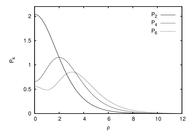
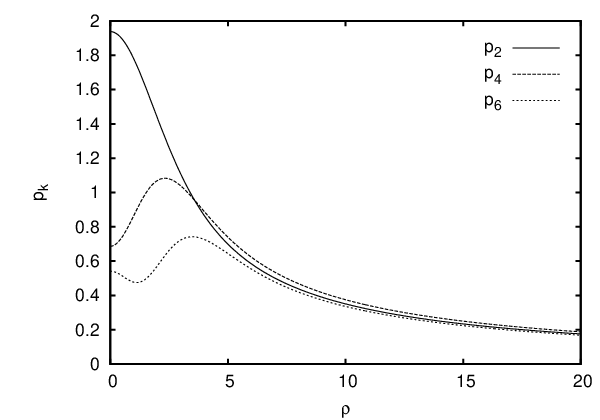
Refer to caption — Figure 1: The first three $P_{k}$ functions for the free scalar field case in $D=3$ spatial dimensions.

The obtained central values of $P_{i}$ and $p_{i}$ for $i=2,4,6$ in $D=3,4,5$ are collected in Table 1.

	$D=3$	$D=4$	$D=5$
$P_{2c}$	2.04299	7.08429	28.0399
$p_{2c}$	1.93832	4.42976	14.90729
$P_{4c}$	0.658158	-5.93174	-348.868
$p_{4c}$	0.686532	-4.08270	-200.353
$P_{6c}$	0.557141	27.3950	9532.72
$p_{6c}$	0.541339	17.9090	5500.18

Table 1: Central values of the first three functions

P_{i}

and

p_{i}

for the free scalar field in

3

4

and

5

spatial dimensions.

The chosen central values make all functions $P_{i}$ and $p_{i}$ , and consequently $\Phi_{i}$ and $\varphi_{i}$ , tend to zero for $\rho\to\infty$ . Although for $i\geq 4$ $P_{i}$ and $p_{i}$ are not monotonically decreasing functions, their central values represent well the magnitude of these functions. Generally, the validity domain of an asymptotic series ends where a higher order term starts giving larger contributions than previous order terms. For $D=3$ the sixth order $\varepsilon$ expansion can be expected to be valid even for as large parameter values as $\varepsilon=1$ . For $D=4$ this domain is $\varepsilon<0.7$ , while for $D=5$ it decreases to $\varepsilon<0.22$ .

3.5 $\varepsilon^{4}$ order for $D=6$

As we have already stated in Subsection 3.1, if $D=6$ then $\omega_{2}=0$ , $s=S$ and the explicit form of the solution of the SN equations is given by (30). Introducing the new variables $z$ and $Z$ by

P_{4}=\frac{1}{3}(2Z+z)\,,\qquad p_{4}+\omega_{4}=\frac{1}{3}(Z-z)\,,

(51)

equations (44) and (45) decouple,

	$\displaystyle\frac{d^{2}z}{d\rho^{2}}+\frac{5}{\rho}\,\frac{dz}{d\rho}-sz+\frac{3}{4}\beta_{1}s^{3}$	$\displaystyle=$	$\displaystyle 0\,,$		(52)
	$\displaystyle\frac{d^{2}Z}{d\rho^{2}}+\frac{5}{\rho}\,\frac{dZ}{d\rho}+2sZ-\frac{9}{4}\beta_{2}s^{3}$	$\displaystyle=$	$\displaystyle 0\,,$		(53)

where the constants $\beta_{1}$ and $\beta_{2}$ are defined by the coefficients in the potential as

	$\displaystyle\beta_{1}$	$\displaystyle=$	$\displaystyle 1+\frac{80}{9}g_{2}^{2}-8g_{3}\,,$		(54)
	$\displaystyle\beta_{2}$	$\displaystyle=$	$\displaystyle 1-\frac{80}{27}g_{2}^{2}+\frac{8}{3}g_{3}\,.$		(55)

For a free scalar field with $U(\Phi)=\Phi^{2}/2$ we have $\beta_{1}=\beta_{2}=1$ . The general regular solution of (52) can be written in terms of the (complex indexed) associated Legendre function $P$ as

z=\frac{144\beta_{1}\alpha^{4}(14+6\alpha^{2}\rho^{2}+\alpha^{4}\rho^{4})}{13(1+\alpha^{2}\rho^{2})^{4}}+\frac{C_{1}}{\alpha^{2}\rho^{2}}P_{(i\sqrt{23}-1)/2}^{2}\left(\frac{1-\alpha^{2}\rho^{2}}{1+\alpha^{2}\rho^{2}}\right)\,,

(56)

where $C_{1}$ is some constant. The limiting value at $\rho\to\infty$ is $z_{\infty}=-C_{1}\cosh(\pi\sqrt{23}/2)/\pi\approx-297.495\,C_{1}$ . The regular solution of (53) is

	$\displaystyle Z$	$\displaystyle=$	$\displaystyle\frac{3888\beta_{2}\alpha^{4}(1-\alpha^{2}\rho^{2})}{7(1+\alpha^{2}\rho^{2})^{3}}\ln(1+\alpha^{2}\rho^{2})$		(57)
			$\displaystyle+\frac{324\beta_{2}\alpha^{6}\rho^{2}(220+100\alpha^{2}\rho^{2}-16\alpha^{4}\rho^{4}-\alpha^{6}\rho^{6})}{35(1+\alpha^{2}\rho^{2})^{4}}+C_{2}\frac{\alpha^{2}\rho^{2}-1}{(\alpha^{2}\rho^{2}+1)^{3}}\,,$		(57)

The limiting value at $\rho\to\infty$ is $Z_{\infty}=-324\beta_{2}\alpha^{4}/35$ , independently of $C_{2}$ . Since $P_{4}$ must tend to zero, according to (51), $z_{\infty}=648\beta_{2}\alpha^{4}/35$ , fixing the constant $C_{1}$ . Since the mass of the field $\Phi$ is intended to remain $m=1$ , the limit of $p_{4}$ also has to vanish, giving

\omega_{4}=-\frac{324}{35}\beta_{2}\alpha^{4}\,.

(58)

This expression is not enough to fix $\omega_{4}$ yet, since $\alpha$ is a free parameter. If $\beta_{2}>0$ then it is reasonable to use (58) to set $\omega_{4}=-1$ , thereby fixing the free parameter $\alpha$ in the $\varepsilon^{2}$ order component of $\Phi$ and $\varphi$ . The change of the so far undetermined constant $C_{2}$ corresponds to a small rescaling of the parameter $\alpha$ in the expression (30). Its concrete value will fix the coefficient $\omega_{6}$ in the expansion of the frequency. The homogeneous parts of the differential equations at higher $\varepsilon$ order will have the same structure as those for $P_{4}$ and $p_{4}$ . Choosing the appropriate homogeneous solutions all higher $\omega_{k}$ components can be set to zero, yielding

\omega=\sqrt{1-\varepsilon^{4}}\ \ {\rm for}\ \ D=6\ \ {\rm if}\ \ \beta_{2}>0\,.

(59)

This expression is valid for the free scalar field case with potential $U(\Phi)=\Phi^{2}/2$ in $D=6$ , since then $\beta_{2}=1$ . For certain potentials $\beta_{2}<0$ , and one can use (58) to set $\omega_{4}=1$ . This case is quite unusual in the sense that the frequency of the oscillon state is above the fundamental frequency $m=1$ . In the very special case, when $\beta_{2}=0$ the frequency differs from the fundamental frequency only in $\varepsilon^{6}$ or possibly higher order terms.

3.6 Total energy and dilaton charge of oscillons

Substituting (47) and (48) into the expression (3) of the total energy, we get

E=\varepsilon^{4-D}E_{0}+\varepsilon^{6-D}E_{1}+\mathcal{O}(\varepsilon^{8-D})\,,

(60)

where

E_{0}=\frac{\pi^{D/2}}{\Gamma(D/2)}\int_{0}^{\infty}d\rho\,\rho^{D-1}P_{2}^{2}\,,\qquad E_{1}=\frac{\pi^{D/2}}{\Gamma(D/2)}\int_{0}^{\infty}d\rho\,\rho^{D-1}P_{2}(2P_{4}-P_{2})\,.

(61)

Since $P_{2}=2S$ , for $2<D<6$ we can use (32) and (33) to get

E_{0}=\frac{4\pi^{D/2}}{\Gamma(D/2)}(D-2)s_{1}\,.

(62)

The numerical values of $s_{1}$ , $E_{0}$ and $E_{1}$ for $D=3,4,5$ are listed in Table 2.

	$D=3$	$D=4$	$D=5$
$s_{1}$	3.50533	7.69489	10.4038
$E_{0}$	88.0985	607.565	1642.91
$E_{1}$	123.576	2522.10	31374.2

Table 2: The numerical values of

s_{1}

E_{0}

and

E_{1}

3

4

and

5

spatial dimensions.

To the calculated order, i.e. up to $\varepsilon^{6-D}$ , for $D=3$ and $D=4$ the energy is a monotonically increasing function of $\varepsilon$ , while for $D=5$ there is an energy minimum at $\varepsilon=0.2288$ . This result can only be taken as an estimate, as the validity domain of an asymptotic series ends when two subsequent terms are approximately equal.

For $D=6$ the leading order term in the total energy is

E=\frac{192\pi^{3}}{\alpha^{2}\varepsilon^{2}}\,.

(63)

As we have already noted, for $D>6$ there are no finite energy solutions.

The leading order $\varepsilon$ dependence of the dilaton charge for $2<D<6$ is given by

Q=s_{1}\varepsilon^{4-D}\,,

(64)

where we used the definition (7), (32) and the relation $\rho=\varepsilon r$ . The dilaton charge for the $D=6$ oscillon is infinite. In higher orders in $\varepsilon$ the proportionality between the dilaton charge and energy is violated.

4 Time evolution of oscillons

In this section we employ a numerical time evolution code in order to simulate the actual behaviour of oscillons in the scalar-dilaton theory. We use a fourth order method of line code with spatial compactification in order to investigate spherically symmetric fields [46]. Our aim is to find configurations which are as closely periodic as possible. To achieve this, we use initial data obtained from the leading $\varepsilon^{2}$ terms of the small amplitude expansion (47) and (48). The smaller the chosen $\varepsilon$ is, the more closely periodic the resulting oscillating state becomes. However, for moderate values of $\varepsilon$ , it is possible to improve the initial data by simply multiplying it by some overall factor very close to $1$ .

The main characteristics of the evolution of small amplitude initial data depend on the number of spatial dimensions $D$ . For $D=3$ and $D=4$ oscillons appear to be stable. If there is some moderate error in the initial data, it will still evolve into an extremely long living oscillating configuration, but its amplitude and frequency will oscillate with a low frequency modulation. We employ a fine-tuning procedure to minimize this modulation by multiplying the initial data with some empirical factor. For $D=5$ and $D=6$ small amplitude oscillons are not stable, having a single decay mode. In this case we can use the fine-tuning method to suppress this decay mode, and make long living oscillon states with well defined amplitude and frequency. Without tuning in $D=5$ and $D=6$ , in general, an initial data evolves into a decaying state. The tuning becomes possible because there are two possible ways of decay. One with a steady outwards flux of energy, the other is through collapsing to a central region first.

Having calculated several closely periodic oscillon configurations, it is instructive to see how closely their total energy follow the expressions (60)-(63). Apart from checking the consistency of the small amplitude and the time-evolution approaches, this also gives information on how large $\varepsilon$ values the small amplitude expansion remains valid. The parameter $\varepsilon$ for the evolving oscillon is calculated from the numerically measured frequency by the expression $\varepsilon=\sqrt{1-\omega^{2}}$ . The results for $D=3$ are presented on Fig. 3.

In contrast to general relativistic oscillatons, there is no maximum on the energy curve. This indicates that all three dimensional oscillons in the dilaton theory are stable.

The $\varepsilon$ dependence of the energy for $D=5$ is presented on Fig. 4.

There is an energy minimum of the numerically obtained states, approximately at $\varepsilon=0.21$ , above which oscillons are stable. The place of the minimum agrees quite well with the value $\varepsilon=0.2288$ calculated in Subsection 3.6 using the first two terms of the small amplitude expansion. The behaviour of the energy close to the minimum is shown on Fig. 5.

We have also constructed oscillon states for $D=6$ dimensions. These oscillons have quite large energy, due to the slow spatial decay of the functions $\Phi$ and $\varphi$ . For free massive scalar fields, oscillons have frequency given by (59), i.e. an initial data with a given $\varepsilon$ value will evolve to an oscillon state with frequency approximately following $\omega=\sqrt{1-\varepsilon^{4}}$ . However, there are potentials, for which the oscillation frequency is above the threshold $\omega=1$ . For example, this happens for the potential $U(\Phi)=\Phi^{2}(\Phi-2)^{2}/8$ with the choice $\kappa=1/2$ .

In conclusion, in the dilaton-scalar theory oscillons follow the stability pattern observed in the case of self-interacting scalar and Einstein-Klein-Gordon theory; if $\varepsilon$ decreases with decreasing energy, oscillons are stable, while if $\varepsilon$ increases with decreasing energy, oscillons are unstable. In other words if the time evolution (i.e. energy loss) of an oscillon leads to spreading of the core, the oscillon is stable, while oscillons are unstable, if they have to contract with time evolution. The decreasing or increasing nature of the energy, and hence empirically the stability of the oscillating configurations, is well described by the first two terms of the small amplitude expansion (60). The result following from Eq. (60) shows the existence of an energy minimum for $D>4$ . This provides an analytical argument for the existence of at least one unstable mode. In particular, for $D=5$ spatial dimensions the frequency separating the stable and unstable domains is determined by the small amplitude expansion to satisfactory precision.

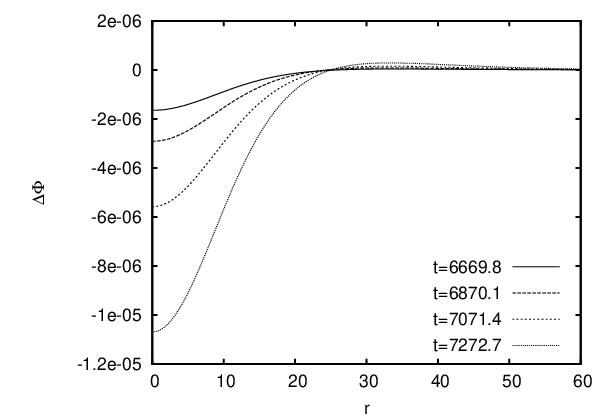
In order to study the instability in more detail numerically, we compared the evolution of two almost identical initial data obtained from the small amplitude expansion with $\varepsilon=0.05$ . In order to make the unstable state long living, a fine tuning procedure is applied, multiplying the amplitude of the initial data by a factor with value close to $1.0178$ . The multiplicative factors used in the two chosen initial values differ by $2.2\times 10^{-16}$ . One of the two initial data develops into a configuration decaying with a uniform outward current of energy, the other through collapsing to a high density state first. On Fig. 6 the time evolution of the difference of the central value of the dilaton fields in the two states $\Delta\varphi=\varphi_{1}-\varphi_{2}$ is shown.

The curve follows extremely well the exponential increase described by

\Delta\varphi=6.583\times 10^{-16}\exp(0.003157\,t)\,,

(65)

showing that there is a single decay mode growing exponentially. The difference of the scalar fields, $\Delta\Phi=\Phi_{1}-\Phi_{2}$ , grows with the same exponent. The spatial dependence of the decaying mode is illustrated on Fig. 7, where $\Delta\Phi$ is plotted at several moments of time corresponding to the maximum of $\Phi_{1}$ at the center.

Our numerical results strongly indicate that oscillons in the scalar-dilaton theory are unstable for $D>4$ , and they admit a single decay mode. For the single scalar field system the instability arises for $D>2$ (see Ref. [31]), but the decay modes have been calculated analytically only in some very special cases. The scalar theory with potential $U(\phi)=\phi^{2}(1-\ln\phi^{2})$ admits exactly time-periodic breathers in any dimensions. The stability of these breathers in three dimensions has been investigated in detail in [47][48]. It has been found that these breathers always admit a single unstable mode. It needs further studies whether an analysis along the lines of Ref. [47] can also be applied to more general potentials in the small amplitude limit, and whether it can be generalized to the case when the scalar is coupled to a dilaton field.

5 Determination of the energy loss rate

Although oscillons are extremely long living, generally they are not exactly periodic. In this section we calculate how the energy loss rate depends on the oscillon frequency for small amplitude configurations. To simplify the expressions in this section we consider a massive free scalar field, i.e. $U(\Phi)=m^{2}\Phi^{2}/2$ . We assume that $2<D<6$ , since then the scalar field tends to zero exponentially for large $\rho$ .

The outgoing radiation will dominantly be in the dilaton field and the radiation amplitude will have the $\varepsilon$ dependence: $\varepsilon\,\exp\left(-2Q_{D}/\varepsilon\right)$ . In Refs. [30] and [31] we have used two different methods for determining the $\varepsilon$ independent part of the radiation amplitude: Borel summation and solution of the complexified mode equations numerically. In this paper we will use an analytic method based on Borel-summing the asymptotic series in the neighborhood of its singularity in the complex plane. Other potentials which are symmetric around their minima can be treated analogously. If the potential is asymmetric only the numerical method could be used. This phenomenon is in complete analogy with the problem arising with a single scalar field considered in Ref. [30].

5.1 Singularity of the small $\varepsilon$ expansion

We first investigate the complex extension of the functions obtained by the small amplitude expansion in Sec. 3. Extending the solutions $s$ and $S$ of the Schrödinger-Newton equations (27) and (28) to complex $\rho$ coordinates they both have pole singularities on the imaginary axis of the complex plane. We consider the closest pair of singularities to the real axis, since these will give the dominant contribution to the energy loss. They are located at $\rho=\pm iQ_{D}$ . The numerically calculated values of $Q_{D}$ are listed in Table 3 for spatial dimensions $D=3,4,5$ .

$\ \ \ D\ \ \$	$\ \ \ \ \ Q_{D}\ \ \ \ \$
3	3.97736
4	2.30468
5	1.23595

Table 3: The distance

Q_{D}

between the real axis and the pole of the fundamental solution of the SN equation for various spatial dimensions

D

Let us measure distances from the upper singularity by a coordinate $R$ defined as

\rho=iQ_{D}+R\,.

(66)

Close to the pole we can expand the SN equations, and obtain that $s$ and $S$ have essentially the same behaviour,

s=\pm S=-\frac{6}{R^{2}}-\frac{6i(D-1)}{5Q_{D}R}-\frac{(D-1)(D-51)}{50Q_{D}^{2}}+{\cal O}(R)\ ,

(67)

even though they clearly differ on the real axis. Since for symmetric potentials we can always substitute $\Phi$ by $-\Phi$ , we choose the positive sign for $S$ in (67). This choice is compatible with the sign of $S$ used on the real axis at the small amplitude expansion section. We note that for $D>1$ there are logarithmic terms in the expansion of $s$ and $S$ , starting with terms proportional to $R^{4}\ln R$ . According to (26), the functions determining the leading $\varepsilon^{2}$ parts of $\varphi$ and $\Phi$ in this case are

p_{2}=s+1\,,\qquad P_{2}=2S\,.

(68)

Substituting these into the equations (44) and (45), the $\varepsilon^{4}$ order contributions $p_{4}$ and $P_{4}$ can also be expanded around the pole

	$\displaystyle p_{4}$	$\displaystyle=$	$\displaystyle-\frac{1161}{52R^{4}}+\frac{324i(D-1)\ln R}{35Q_{D}R^{3}}+\frac{c_{-3}}{R^{3}}+{\cal O}\left(\frac{\ln R}{R^{2}}\right)$		(69)
	$\displaystyle P_{4}-2p_{4}$	$\displaystyle=$	$\displaystyle\frac{81}{13R^{4}}+\frac{18i(D-1)}{5Q_{D}R^{3}}+{\cal O}\left(\frac{1}{R^{2}}\right)\,,$		(70)

where the constant $c_{-3}$ can only be determined from the specific behaviour of the functions on the real axis, namely from the requirement of the exponential decay of $P_{4}$ for large real $\rho$ .

5.2 Fourier mode expansion

Since all terms of the small amplitude expansion (9) are asymptotically decaying, i.e. localized functions, the small amplitude expansion can be successfully applied to the core region of oscillons. However it cannot describe the exponentially small radiative tail responsible for the energy loss. Instead of studying a slowly varying frequency radiating oscillon configuration it is simpler to consider exactly periodic solutions having a large core and a very small amplitude standing wave tail. We look for periodic solutions with frequency $\omega$ by Fourier expanding the scalar and dilaton field as

\Phi=\sum_{k=0}^{N_{F}}\Psi_{k}\cos(k\omega t)\,,\qquad\varphi=\sum_{k=0}^{N_{F}}\psi_{k}\cos(k\omega t)\,.

(71)

Although, in principle, the Fourier truncation order $N_{F}$ should tend to infinity, one can expect very good approximation for moderate values of $N_{F}$ . In (71) we denoted the Fourier components by psi instead of phi to distinguish them from the small $\varepsilon$ expansion components in (9). Since in this section we only deal with an self-interaction free scalar field with a trivially symmetric potential,

\Psi_{2k}=0\,,\qquad\psi_{2k+1}=0\,,\qquad{\rm for\ integer}\ k\,.

(72)

We note that the absence of sine terms in (71) is equivalent to the assumption of time reflexion symmetry at $t=0$ . This assumption appears reasonable physically, and we have seen in Sec. 3 that it holds in the small amplitude expansion framework.

For small amplitude configurations we can establish the connection between the expansions (9) and (71) by comparing to (47) and (48), obtaining

$\displaystyle\Psi_{1}$	$\displaystyle=$	$\displaystyle\varepsilon^{2}P_{2}+\varepsilon^{4}P_{4}+\varepsilon^{6}P_{6}+{\cal O}(\varepsilon^{8})\ ,$	(73)
$\displaystyle\Psi_{3}$	$\displaystyle=$	$\displaystyle\varepsilon^{6}\frac{P_{2}^{3}}{256}+{\cal O}(\varepsilon^{8})\ ,$	(74)
$\displaystyle\psi_{0}$	$\displaystyle=$	$\displaystyle\varepsilon^{2}p_{2}+\varepsilon^{4}p_{4}+\varepsilon^{6}p_{6}+{\cal O}(\varepsilon^{8})\ ,$	(75)
$\displaystyle\psi_{2}$	$\displaystyle=$	$\displaystyle-\varepsilon^{4}\frac{P_{2}^{2}}{16}-\varepsilon^{6}\frac{1}{32}\left[4P_{2}P_{4}-(p_{2}-1)P_{2}^{2}-\left(\frac{dP_{2}}{dR}\right)^{2}\right]+{\cal O}(\varepsilon^{8})\ .$	(76)

Let us define a coordinate $y$ for an “inner region” by $R=\varepsilon y$ . This coordinate will have the same scale as the original radial coordinate $r$ , since they are related as

r=\frac{iQ_{D}}{\varepsilon}+y\,.

(77)

The “inner region” $|R|\ll 1$ is not small in the $y$ coordinate; if $\varepsilon\to 0$ then $\varepsilon|y|=|R|\ll 1$ but $|y|\to\infty$ . Using the coordinate $y$ and substituting (67)-(70) into the small amplitude Fourier mode expressions (73)-(76), we obtain that the leading asymptotic behaviour of the Fourier modes for $|y|\to\infty$ can be written as

$\displaystyle\Psi_{1}$	$\displaystyle=$	$\displaystyle-\frac{12}{y^{2}}-\frac{999}{26y^{4}}+\varepsilon\ln\varepsilon\frac{648i(D-1)}{35Q_{D}y^{3}}$	(78)
		$\displaystyle+\varepsilon\left[\frac{6i(D-1)}{5Q_{D}y}\left(\frac{3}{y^{2}}+\frac{108\ln y}{7y^{2}}-2\right)+\frac{2c_{-3}}{y^{3}}\right]+\ldots\ ,$	(78)
$\displaystyle\Psi_{3}$	$\displaystyle=$	$\displaystyle-\frac{27}{4y^{6}}-\varepsilon\frac{81i(D-1)}{20Q_{D}y^{5}}+\ldots\ ,$	(79)
$\displaystyle\psi_{0}$	$\displaystyle=$	$\displaystyle-\frac{6}{y^{2}}-\frac{1161}{52y^{4}}+\varepsilon\ln\varepsilon\frac{324i(D-1)}{35Q_{D}y^{3}}$	(80)
		$\displaystyle+\varepsilon\left[\frac{6i(D-1)}{5Q_{D}y}\left(\frac{54\ln y}{7y^{2}}-1\right)+\frac{c_{-3}}{y^{3}}\right]+\ldots\ ,$	(80)
$\displaystyle\psi_{2}$	$\displaystyle=$	$\displaystyle-\frac{9}{y^{4}}-\varepsilon\frac{18i(D-1)}{5Q_{D}y^{3}}+\ldots\ .$	(81)

These expressions are simultaneous series in $1/y$ and in $\varepsilon$ .

5.3 Fourier mode equations

In order to obtain finite number of Fourier mode equations with finite number of terms, when substituting (71) into the field equations (5) and (6) we Taylor expand and truncate the exponential

e^{-\varphi}=\sum_{k=0}^{N_{e}}\frac{1}{k!}(-\varphi)^{k}\,.

(82)

We need to carefully check how large $N_{e}$ should be chosen to have only a negligible influence to the calculated results. For $n\leq N_{F}$ the Fourier mode equations have the form

	$\displaystyle\left(\frac{\mathrm{d^{2}}}{\mathrm{d}r^{2}}+\frac{D-1}{r}\,\frac{\mathrm{d}}{\mathrm{d}r}+n^{2}\omega^{2}-1\right)\Psi_{n}$	$\displaystyle=$	$\displaystyle F_{n}\ ,$		(83)
	$\displaystyle\left(\frac{\mathrm{d^{2}}}{\mathrm{d}r^{2}}+\frac{D-1}{r}\,\frac{\mathrm{d}}{\mathrm{d}r}+n^{2}\omega^{2}\right)\psi_{n}$	$\displaystyle=$	$\displaystyle f_{n}\ ,$		(84)

where we have collected the nonlinear terms to the right hand sides, and denoted them with $F_{n}$ and $f_{n}$ . These are polynomial expressions involving various $\Psi_{k}$ and $\psi_{k}$ , with quickly increasing complexity when increasing the truncation orders $N_{F}$ and $N_{e}$ . The solution of (83) and (84) yields the intended quasibreathers, with a localized core and a very small amplitude oscillating tail. For small amplitude configurations the functions $\Psi_{k}$ and $\psi_{k}$ will have poles at the complex $r$ plane, just as we have seen in the small amplitude expansion formalism. In order to calculate the tail amplitude it is necessary to investigate the Fourier mode equations instead of the equations obtained in Sec. 3. Although in the Fourier decomposition method we have not defined a small amplitude parameter yet, motivated by (38), we can, in general, define $\varepsilon$ as

\varepsilon=\sqrt{1-\omega^{2}}\,.

(85)

Dropping $\mathcal{O}(\varepsilon^{2})$ terms, in the neighborhood of the singularity the mode equations take the form

	$\displaystyle\left(\frac{\mathrm{d^{2}}}{\mathrm{d}y^{2}}+\varepsilon\frac{D-1}{iQ_{D}}\,\frac{\mathrm{d}}{\mathrm{d}y}+n^{2}-1\right)\Psi_{n}$	$\displaystyle=$	$\displaystyle F_{n}\ ,$		(86)
	$\displaystyle\left(\frac{\mathrm{d^{2}}}{\mathrm{d}y^{2}}+\varepsilon\frac{D-1}{iQ_{D}}\,\frac{\mathrm{d}}{\mathrm{d}y}+n^{2}\right)\psi_{n}$	$\displaystyle=$	$\displaystyle f_{n}\ .$		(87)

We look for solutions of these equations that satisfy (78)-(81) as boundary conditions for $|y|\to\infty$ for $-\pi/2<\arg y<0$ . This corresponds to the requirement that the functions decay to zero without any oscillating tails for large $r$ on the real axis. The small correction corresponding to the nonperturbative tail of the quasibreather will arise in the imaginary part of the functions on the $\textrm{Re}\,y=0$ axis.

5.4 $\varepsilon\to 0$ limit near the pole

For very small $\varepsilon$ values one can neglect the terms proportional $\varepsilon$ on the left hand sides of (86) and (87). In this limit the there is no dependence on the number of spatial dimensions $D$ . We investigate this simpler system first, and consider finite but small $\varepsilon$ corrections later as perturbations to it. We expand the solution of (86) and (87) (with $\varepsilon=0$ ) in even powers of $1/y$ ,

\Psi_{2k+1}=\sum_{j=k+1}^{\infty}A_{2k+1}^{(j)}\frac{1}{y^{2j}}\,,\qquad\psi_{2k}=\sum_{j=k+1}^{\infty}a_{2k}^{(j)}\frac{1}{y^{2j}}\,.

(88)

We illustrate our method by a minimal system where radiation loss can be studied, namely the case with $N_{F}=3$ and $N_{e}=1$ . Then the mode equations are still short enough to print:

$\displaystyle\frac{d^{2}\psi_{0}}{dy^{2}}$	$\displaystyle=$	$\displaystyle\frac{1}{4}(\psi_{0}-1)(\Psi_{1}^{2}+\Psi_{3}^{2})+\frac{1}{8}\psi_{2}\Psi_{1}(\Psi_{1}+2\Psi_{3})\,,$	(89)
$\displaystyle\frac{d^{2}\Psi_{1}}{dy^{2}}$	$\displaystyle=$	$\displaystyle-\psi_{0}\Psi_{1}-\frac{1}{2}\psi_{2}(\Psi_{1}+\Psi_{3})\,,$	(90)
$\displaystyle\frac{d^{2}\psi_{2}}{dy^{2}}+4\psi_{2}$	$\displaystyle=$	$\displaystyle\frac{1}{4}\Psi_{1}(\psi_{0}-1)(\Psi_{1}+2\Psi_{3})+\frac{1}{4}\psi_{2}(\Psi_{1}^{2}+\Psi_{1}\Psi_{3}+\Psi_{3}^{2})\,,$	(91)
$\displaystyle\frac{d^{2}\Psi_{3}}{dy^{2}}+8\Psi_{3}$	$\displaystyle=$	$\displaystyle-\frac{1}{2}\psi_{2}\Psi_{1}-\psi_{0}\Psi_{3}\,.$	(92)

When looking for solution of these equations in the form of the $1/y^{2}$ expansion (88), only one ambiguity arises, the sign of $A_{0}^{(1)}$ . Choosing it to be negative, the first few terms of the expansion turn out to be

$\displaystyle\psi_{0}$	$\displaystyle=$	$\displaystyle-\frac{6}{y^{2}}-\frac{837}{52y^{4}}+\mathcal{O}\left(\frac{1}{y^{6}}\right)\,,$	(93)
$\displaystyle\Psi_{1}$	$\displaystyle=$	$\displaystyle-\frac{12}{y^{2}}-\frac{459}{26y^{4}}+\mathcal{O}\left(\frac{1}{y^{6}}\right)\,,$	(94)
$\displaystyle\psi_{2}$	$\displaystyle=$	$\displaystyle-\frac{9}{y^{4}}-\frac{1845}{52y^{6}}+\mathcal{O}\left(\frac{1}{y^{8}}\right)\,,$	(95)
$\displaystyle\Psi_{3}$	$\displaystyle=$	$\displaystyle-\frac{27}{4y^{6}}-\frac{2565}{416y^{8}}+\mathcal{O}\left(\frac{1}{y^{10}}\right)\,.$	(96)

The first terms agree with those of (78)-(81) obtained by the small amplitude expansion. The difference in the $1/y^{4}$ terms of $\psi_{0}$ and $\Psi_{1}$ are caused by the too low truncation for the Taylor expansion of the exponential. For $N_{e}\geq 2$ these terms agree as well.

When increasing $N_{F}$ and $N_{e}$ growing number of additional terms appear on the right hand sides of (89)-(92), and the number of mode equations rise to $N_{F}+1$ . These complicated mode equations can be calculated and $1/y^{2}$ expanded using an algebraic manipulation program. However, apart from a factor, the leading order behaviour of the coefficients $a_{2}^{(n)}$ and $A_{3}^{(n)}$ for large $n$ will remain the same as that of the minimal system (89)-(92). The large $n$ behaviour of these coefficients will be essential for the calculation of the nonperturbative effects resulting in radiation loss for oscillons.

Starting from the free system, consisting of the linear terms on the left hand sides, it is easy to see that the mode equations are consistent with the following asymptotic (large $n$ ) behavior of the coefficients,

	$\displaystyle a_{2}^{(n)}$	$\displaystyle\sim$	$\displaystyle k\,(-1)^{n}\,\frac{(2n-1)!}{4^{n}}$		(97)
	$\displaystyle a_{0}^{(n)},\,A_{1}^{(n)},\,A_{3}^{(n)}\,$	$\displaystyle\ll$	$\displaystyle a_{2}^{(n)}\,,$		(98)

where $k$ is some constant. The value of $k$ can be obtained to a satisfactory precision by substituting the $1/y$ expansion into the mode equations and explicitly calculating the coefficients to up to high orders in $n$ . In practice, using an algebraic manipulation software, we have calculated coefficients up to order $n=50$ . The dependence of $k$ on the order of the Fourier expansion is given in Table 4.

$N_{F}$	$N_{e}^{(min)}$	$k$
$3$	$5$	$3.71\times 10^{-3}$
$4$	$7$	$3.12\times 10^{-6}$
$5$	$8$	$6.03\times 10^{-9}$
$6$	$10$	$4.61\times 10^{-13}$

Table 4: Dependence of the constant

k

on the considered Fourier components

N_{F}

. The second column lists the minimal exponential expansion order

N_{e}

which is necessary to get the

k

value with the given precision.

The results strongly indicate that in the $N_{f},N_{e}\to\infty$ limit $k=0$ . We do not yet understand what is the deeper reason or symmetry behind this. Hence, instead of (97) and (98), the correct asymptotic behavior is

	$\displaystyle A_{3}^{(n)}$	$\displaystyle\sim$	$\displaystyle K\,(-1)^{n}\,\frac{(2n-1)!}{8^{n}}$		(99)
	$\displaystyle a_{0}^{(n)},\,A_{1}^{(n)},\,a_{2}^{(n)}\,$	$\displaystyle\ll$	$\displaystyle A_{3}^{(n)}\,.$		(100)

Taking at least $N_{F}=6$ and $N_{e}=9$ , the numerical value of the constant turns out to be $K=-0.57\pm 0.01$ . The above results indicate that the outgoing radiation is in the $\Psi_{3}$ scalar mode instead of being in the $\psi_{2}$ dilaton mode. This conclusion is valid only in the framework of the approximation employed in the present subsection, i.e. when dropping the terms proportional to $\varepsilon$ in (86) and (87). As we will see in the next subsection, the situation will change to be just the opposite when taking into account $\varepsilon$ corrections.

All terms of the expansion (88) are real on the imaginary axis $\mathrm{Re}\,y=0$ . However, using the Borel-summation procedure it is possible to calculate there an exponentially small correction to the imaginary part. We will only sketch how the summation is done, for details see [30] and [37]. We illustrate the method by applying it to $\Psi_{3}$ . The first step is to define a Borel summed series by

V(z)=\sum_{n=2}^{\infty}\frac{A_{3}^{(n)}}{(2n)!}\;z^{2n}\sim\sum_{n=2}^{\infty}K\,\frac{(-1)^{n}}{2n}\;\left(\frac{z}{\sqrt{8}}\right)^{2n}=-\frac{K}{2}\ln\left(1+\frac{z^{2}}{8}\right)\;.

(101)

This series has logarithmic singularities at $z=\pm i\sqrt{8}$ . The Laplace transform of $V(z)$ will give us the Borel summed series of $\Psi_{3}(y)$ which we denote by $\widehat{\Psi}_{3}(y)$

\widehat{\Psi}_{3}(y)=\int_{0}^{\infty}\;\mathrm{d}t\,e^{-t}V\left(\frac{t}{y}\right)\,.

(102)

The choice of integration contour corresponds to the requirement of exponential decay on the real axis. The logarithmic singularity of $V\left(t/y\right)$ does not contribute to the integral and integrating on the branch cut starting from it yields the imaginary part

{\rm Im}\,\widehat{\Psi}_{3}(y)=\int_{i\sqrt{8}\,y}^{\infty}\;\mathrm{d}t\;e^{-t}\,\frac{K\pi}{2}=\frac{K\pi}{2}\,\exp\left(-i\sqrt{8}\,y\right)\,.

(103)

A similar calculation for the $\psi_{2}$ dilaton mode yields

{\rm Im}\,\widehat{\psi}_{2}(y)=\frac{k\pi}{2}\,\exp\left(-2iy\right)\,.

(104)

Since $k=0$ , this mode is vanishing now. However, as we will show in the next subsection, when taking into account order $\varepsilon$ corrections a similar expression for $\psi_{2}$ with $\exp\left(-2iy\right)$ behaviour arise, which, due to its slower decay, will become dominant when $\mathrm{Im}\,y\to-\infty$ . The continuation to the real axis of these imaginary corrections turns out to be closely related to the asymptotically oscillating mode responsible for the slow energy loss of oscillons.

5.5 Order $\varepsilon$ corrections near the pole

Before discussing the issue of matching the imaginary correction calculated in the neighborhood of the singularity to the solution of the field equation on the real axis we deal with the corrections arising when taking into account the terms proportional to $\varepsilon$ in the mode equations (86) and (87). We denote the solutions obtained in the previous subsection by $\psi_{n}^{(0)}$ and $\Psi_{n}^{(0)}$ , and linearize the mode equations around them by defining

\psi_{n}=\psi_{n}^{(0)}+\widetilde{\psi}_{n}\,,\qquad\Psi_{n}=\Psi_{n}^{(0)}+\widetilde{\Psi}_{n}\,.

(105)

The mode equations take the form

	$\displaystyle\left(\frac{{\rm d}^{2}}{{\rm d}y^{2}}+n^{2}\right)\widetilde{\psi}_{n}+\varepsilon\frac{D-1}{iQ_{D}}\,\frac{{\rm d}\psi_{n}^{(0)}}{{\rm d}y}$	$\displaystyle=$	$\displaystyle\sum_{m}\frac{\partial f_{n}}{\partial\psi_{m}}\widetilde{\psi}_{m}+\sum_{m}\frac{\partial f_{n}}{\partial\Psi_{m}}\widetilde{\Psi}_{m}\,,$		(106)
	$\displaystyle\left(\frac{{\rm d}^{2}}{{\rm d}y^{2}}+n^{2}-1\right)\widetilde{\Psi}_{n}+\varepsilon\frac{D-1}{iQ_{D}}\,\frac{{\rm d}\Psi_{n}^{(0)}}{{\rm d}y}$	$\displaystyle=$	$\displaystyle\sum_{m}\frac{\partial F_{n}}{\partial\psi_{m}}\widetilde{\psi}_{m}+\sum_{m}\frac{\partial F_{n}}{\partial\Psi_{m}}\widetilde{\Psi}_{m}\,,$		(107)

where the partial derivatives on the right hand sides are taken at $\Psi_{n}=\Psi_{n}^{(0)}$ and $\psi_{n}=\psi_{n}^{(0)}$ . The small dimensional corrections $\widetilde{\psi}_{n}$ and $\widetilde{\Psi}_{n}$ have parts of order both $\varepsilon\ln\varepsilon$ and $\varepsilon$ .

The linearized equations (106) and (107) are solved to $\varepsilon\ln\varepsilon$ order by the following functions:

	$\displaystyle\widetilde{\psi}_{n}$	$\displaystyle=$	$\displaystyle\varepsilon\ln\varepsilon\,C\frac{{\rm d}\psi_{n}^{(0)}}{{\rm d}y}\,,$		(108)
	$\displaystyle\widetilde{\Psi}_{n}$	$\displaystyle=$	$\displaystyle\varepsilon\ln\varepsilon\,C\frac{{\rm d}\Psi_{n}^{(0)}}{{\rm d}y}\,,$		(109)

where $C$ is an arbitrary constant. The reason for this is quite simple: in $\varepsilon\ln\varepsilon$ order the terms proportional to $\varepsilon$ on the left hand sides are negligible and we get the $\varepsilon=0$ equation linearized about the original solution. Our formula simply gives the zero mode of this equation. The constant $C$ is determined by the appropriate behaviour when continuing back our functions to the real axis. This can be ensured by requiring agreement with the first few terms of the small amplitude expansion formulae (78)-(81), yielding

C=\frac{27i(D-1)}{35Q_{D}}\,.

(110)

In the small amplitude expansion (78)-(81) to every term of order $\varepsilon\ln\varepsilon$ corresponds a term of order $\varepsilon$ which we get by changing $\ln\varepsilon$ to $\ln y$ . Thus, we define the new variables $\overline{\psi}_{n}$ and $\overline{\Psi}_{n}$ to describe the $\varepsilon$ order small perturbations by

	$\displaystyle\widetilde{\psi}_{n}$	$\displaystyle=$	$\displaystyle\varepsilon\ln\varepsilon\,C\frac{{\rm d}\psi_{n}^{(0)}}{{\rm d}y}+\varepsilon\left(C\ln y\,\frac{{\rm d}\psi_{n}^{(0)}}{{\rm d}y}+\overline{\psi}_{n}\right)\,,$		(111)
	$\displaystyle\widetilde{\Psi}_{n}$	$\displaystyle=$	$\displaystyle\varepsilon\ln\varepsilon\,C\frac{{\rm d}\Psi_{n}^{(0)}}{{\rm d}y}+\varepsilon\left(C\ln y\,\frac{{\rm d}\Psi_{n}^{(0)}}{{\rm d}y}+\overline{\Psi}_{n}\right)\,.$		(112)

Substituting into the linearized equations (106) and (107) we see that all terms containing $\ln y$ cancel out,

	$\displaystyle\left(\frac{{\rm d}^{2}}{{\rm d}y^{2}}+n^{2}\right)\overline{\psi}_{n}+\frac{C}{y^{2}}\left(2y\frac{{\rm d^{2}}\psi_{n}^{(0)}}{{\rm d}y^{2}}-\frac{{\rm d}\psi_{n}^{(0)}}{{\rm d}y}\right)+\frac{D-1}{iQ_{D}}\,\frac{{\rm d}\psi_{n}^{(0)}}{{\rm d}y}=$
	$\displaystyle\qquad=\sum_{m}\frac{\partial f_{n}}{\partial\psi_{m}}\overline{\psi}_{m}+\sum_{m}\frac{\partial f_{n}}{\partial\Psi_{m}}\overline{\Psi}_{m}\,,$		(113)
	$\displaystyle\left(\frac{{\rm d}^{2}}{{\rm d}y^{2}}+n^{2}-1\right)\overline{\Psi}_{n}+\frac{C}{y^{2}}\left(2y\frac{{\rm d^{2}}\Psi_{n}^{(0)}}{{\rm d}y^{2}}-\frac{{\rm d}\Psi_{n}^{(0)}}{{\rm d}y}\right)+\frac{D-1}{iQ_{D}}\,\frac{{\rm d}\Psi_{n}^{(0)}}{{\rm d}y}=$
	$\displaystyle\qquad=\sum_{m}\frac{\partial F_{n}}{\partial\psi_{m}}\overline{\psi}_{m}+\sum_{m}\frac{\partial F_{n}}{\partial\Psi_{m}}\overline{\Psi}_{m}\,.$		(114)

If $C$ is given by (110), $\overline{\psi}_{n}$ and $\overline{\Psi}_{n}$ turn out to be algebraic asymptotic series which are analytic in $y$ . Let us write their expansion explicitly:

\overline{\Psi}_{2k+1}=\sum_{n=k+1}^{\infty}B_{2k+1}^{(n)}\frac{1}{y^{2n-1}}\,,\qquad\overline{\psi}_{2k}=\sum_{n=k+1}^{\infty}b_{2k}^{(n)}\frac{1}{y^{2n-1}}\,.

(115)

Substituting these and the expansions (88) for $\psi_{n}^{(0)}$ and $\Psi_{n}^{(0)}$ into (113) and (114), it is possible to solve for the coefficients $b_{k}^{(n)}$ and $B_{k}^{(n)}$ , up to one free parameter. Comparing to (78)-(81) it is natural to choose this free parameter to be $b_{0}^{(2)}=c_{-3}$ . Similarly to that case, $b_{0}^{(2)}$ will only be determined by the requirement that the extension to the real axis represent a localized solution. Furthermore, leaving $C$ a free constant and requiring the absence of logarithmic terms in the expansion of $\overline{\psi}_{k}$ and $\overline{\Psi}_{k}$ yields exactly the value of $C$ given in (110).

Eq. (113) is consistent with the asymptotics

b_{2}^{(n)}\sim ik_{D}\,(-1)^{n}\,\frac{(2n-2)!}{2^{2n-1}}\left[1+\mathcal{O}\left(\frac{1}{n^{3}}\right)\right],

(116)

where $k_{D}$ is some constant. Since the leading order result for $A_{3}^{(n)}$ is given by (99), if $k_{D}\neq 0$ , the coefficients follow the hierarchy $b_{2}^{(n)}\gg A_{3}^{(n-1)}$ . In order to be able to extract the value of $k_{D}$ we have calculated $b_{2}^{(n)}$ by solving the mode equations to high orders in $1/y$ , obtaining

k_{D}=1.640\,\frac{D-1}{Q_{D}}\,.

(117)

The displayed four digits precision for $k_{D}$ can be relatively easily obtained by setting $N_{F}\geq 4$ , $N_{e}\geq 5$ and calculating $b_{2}^{(n)}$ to orders $n\geq 25$ . We note that there is also a term proportional to the unknown $b_{0}^{(2)}=c_{-3}$ in each $b_{2}^{(n)}$ , giving a $c_{-3}$ dependent $k_{D}$ . Luckily, the influence of this term to $k_{D}$ quickly becomes negligible as $N_{F}$ and $N_{e}$ grow, making the concrete value of $c_{-3}$ irrelevant for our purpose.

The Borel summation procedure can be done similarly as in Eqs. (101)-(103). On the imaginary axis $\psi_{2}$ is real to every order in $1/y$ , however it gets a small imaginary correction from the summation procedure given by

{\rm Im}\,\widehat{\psi}_{2}(y)=\varepsilon\,\frac{k_{D}\pi}{2}\,\exp\left(-2iy\right)\,.

(118)

5.6 Extension to the real axis

Solutions of the Fourier mode equations (83) and (84) can be considered to be the sum of two parts. The first part corresponds to the result of the small amplitude expansion, the second to an exponentially small correction to it. The small amplitude expansion is an asymptotic expansion, it gives better and better approximation until reaching an optimal order, but higher terms give increasingly divergent results. The smaller $\varepsilon$ is, the higher the optimal truncation order becomes, and the precision also improves. The small amplitude expansion procedure gives time-periodic localized regular functions to all orders, characterizing the core part of the quasibreather. Their extension to the complex plane is real on the imaginary axis. Furthermore, the functions obtained by the $\varepsilon$ expansion are smooth on large scales, missing an oscillating tail and short wavelength oscillations in the core region. On the imaginary axis, to a very good approximation, the small second part of the solution of the mode equations (83) and (84) is pure imaginary, and satisfies the homogeneous linear equations obtained by keeping only the left hand sides of these equations, because the quasibreather is a small-amplitude one. In the ”inner region” it is of order $1/y^{2}$ , while on the real axis its amplitude is of order $\varepsilon^{2}$ , hence to leading order the quasibreather core background does not contribute. In the previous subsection we have determined the behaviour of this small correction close to the poles. Now we extend it to the real axis.

In the “inner region”, close to the pole, the function ${\rm Im}\,\widehat{\psi}_{2}$ given by (118) solves the homogeneous linear differential equations given by the left hand side of (87). The extension of this function to the real axis will provide the small correction to the small amplitude result mentioned in the previous paragraph. We intend to find the solution $\widehat{\psi}_{2}$ of the left hand side of (84), which reduces to the value given by (118) close to the upper pole, where $r=iQ_{D}/\varepsilon+y$ , and behaves as

{\rm Im}\,\widehat{\psi}_{2}(y)=-\varepsilon\,\frac{k_{D}\pi}{2}\,\exp\left(2iy\right)\,.

(119)

near the lower pole, where $r=-iQ_{D}/\varepsilon+y$ . We follow the procedure detailed in [31]. The resulting function for large $r$ is

\widehat{\psi}_{2}=\varepsilon\,\frac{ik_{D}\pi}{2}\left(\frac{Q_{D}}{\varepsilon r}\right)^{(D-1)/2}\exp\left(-\frac{2Q_{D}}{\varepsilon}\right)\left[i^{(D-1)/2}\exp(-2ir)-(-i)^{(D-1)/2}\exp(2ir)\right].

(120)

The general solution of the left hand side of (84) can be written as a sum involving Bessel functions $J_{n}$ and $Y_{n}$ , which have the asymptotic behaviour

	$\displaystyle J_{\nu}(x)$	$\displaystyle\to$	$\displaystyle\sqrt{\frac{2}{\pi x}}\,\cos\left(x-\frac{\nu\pi}{2}-\frac{\pi}{4}\right),$		(121)
	$\displaystyle Y_{\nu}(x)$	$\displaystyle\to$	$\displaystyle\sqrt{\frac{2}{\pi x}}\,\sin\left(x-\frac{\nu\,\pi}{2}-\frac{\pi}{4}\right),$		(122)

for $x\to+\infty$ . The solution satisfying the asymptotics given by (120) is

\widehat{\psi}_{2}=\sqrt{\pi}\,\frac{\alpha_{D}}{r^{D/2-1}}Y_{D/2-1}(2r)\,,

(123)

where the amplitude at large $r$ is given by

\alpha_{D}=\varepsilon\pi k_{D}\left(\frac{Q_{D}}{\varepsilon}\right)^{(D-1)/2}\exp\left(-\frac{2Q_{D}}{\varepsilon}\right).

(124)

For $D>2$ the function given by (123) is singular at the center, due to the usual central singularity of spherical waves. Since the amplitude of the quasibreather core is proportional to $\varepsilon^{2}$ , and its size to $1/\varepsilon$ , for small $\varepsilon$ it is possible to extend the function $\widehat{\psi}_{2}$ in its form (123) to the real axis into a region which is outside the domain where $\widehat{\psi}_{2}$ gets large, but which is still close to the center when considering the enlarged size of the quasibreather core. When extending this function further out along the real $r$ axis, because of the large size of the quasibreather core, the nonlinear source terms on the right hand side of (84) are not negligible anymore, and the expression (123) for $\widehat{\psi}_{2}$ cannot be used. What actually happens is that $\widehat{\psi}_{2}$ tends to zero exponentially as $r\to\infty$ . This follows from the special choice of the “inner solution” close to the singularity; namely, we were looking for a solution which agreed with the small amplitude expansion for ${\rm Re}\,y\to\infty$ . The small amplitude expansion gives exponentially localized functions to each order and we also required decay beyond all orders when choosing the contour of integration in the Borel summation procedure.

By the above procedure we have constructed a solution of the mode equations which is singular at $r=0$ . The singularity is the consequence of the initial assumption of exponential decay for large $r$ . The asymptotic decay induces an oscillation given by (123) in the intermediate core, and a singularity at the center. In contrast, the quasibreather solution has a regular center, but contains a minimal amplitude standing wave tail asymptotically. Considering the left hand side of (84) as an equation describing perturbation around the asymptotically decaying solution, we just have to add a solution $\delta\psi_{2}$ determined by the amplitude (124) with the opposite sign of (123) to cancel the oscillation and the singularity in the core. This way one obtains the regular quasibreather solution, whose minimal amplitude standing wave tail is given as

	$\displaystyle\phi_{QB}$	$\displaystyle=$	$\displaystyle-\sqrt{\pi}\,\frac{\alpha_{D}}{r^{D/2-1}}Y_{D/2-1}(2r)\cos(2t)$		(125)
		$\displaystyle\approx$	$\displaystyle-\frac{\alpha_{D}}{r^{(D-1)/2}}\sin\left[2r-(D-1)\frac{\pi}{4}\right]\cos(2t).$		(126)

Adding the regular solution, where $Y$ is replaced by $J$ , would necessarily increase the asymptotic amplitude.

If we subtract the incoming radiation from a QB and cut the remaining tail at large distances, we obtain an oscillon state to a good approximation. Subtracting the regular solution with a phase shift in time, we cancel the incoming radiating component, and obtain the radiative tail of the oscillon,

	$\displaystyle\phi_{osc}$	$\displaystyle=$	$\displaystyle-\sqrt{\pi}\,\frac{\alpha_{D}}{r^{D/2-1}}\left[Y_{D/2-1}(2r)\cos(2t)-J_{D/2-1}(2r)\sin(2t)\right]$		(127)
		$\displaystyle\approx$	$\displaystyle-\frac{\alpha_{D}}{r^{(D-1)/2}}\sin\left[2r-(D-1)\frac{\pi}{4}-2t\right].$		(128)

The radiation law of the oscillon is easily obtained now,

\frac{\mathrm{d}E}{\mathrm{d}t}=-k_{D}^{2}\pi^{2}\,\frac{4\pi^{D/2}}{\Gamma\left(\frac{D}{2}\right)}\,\varepsilon^{2}\left(\frac{Q_{D}}{\varepsilon}\right)^{D-1}\exp\left(-\frac{4Q_{D}}{\varepsilon}\right),

(129)

where the constant $k_{D}$ is given by (117). If we assume adiabatic time evolution of the $\varepsilon$ parameter determining the oscillon state, using Eqs. (60) and (62) giving $E$ as a function of $\varepsilon$ , we get a closed evolution equation for small amplitude oscillons, determining their energy as the function of time.

For the physically most interesting case, $D=3$ we write the evolution equation for $\varepsilon$ and its leading order late time behavior explicitly:

	$\displaystyle\frac{\mathrm{d}\varepsilon}{\mathrm{d}t}$	$\displaystyle=$	$\displaystyle-30.29\,\exp\left(-\frac{15.909}{\varepsilon}\right)$		(130)
	$\displaystyle\varepsilon$	$\displaystyle\approx$	$\displaystyle\frac{15.909}{\ln t}\,,\quad E\approx\frac{1401.6}{\ln t}\,.$		(131)

6 Acknowledgments

This research has been supported by OTKA Grants No. K61636, NI68228.

References

[1] R. F. Dashen, B. Hasslacher and A. Neveu, Phys. Rev. D 11, 3424 (1975).
[2] A. E. Kudryavtsev, JETP Letters 22, 82 (1975).
[3] I. L. Bogolyubskii, and V. G. Makhan’kov, JETP Letters 25, 107 (1977).
[4] V. G. Makhankov, Physics Reports 35, 1-128 (1978).
[5] J. Geicke, Physica Scripta 29, 431 (1984).
[6] M. Gleiser, Phys. Rev. D 49, 2978 (1994).
[7] E. J. Copeland, M. Gleiser and H.-R. Müller, Phys. Rev. D 52, 1920 (1995).
[8] M. Gleiser and A. Sornborger, Phys. Rev. E 62, 1368 (2000).
[9] E. P. Honda and M. W. Choptuik, Phys. Rev. D 65, 084037 (2002).
[10] M. Gleiser Phys. Lett. B 600, 126 (2004).
[11] M. Hindmarsh and P. Salmi, Phys. Rev. D 74, 105005 (2006).
[12] G. Fodor, P. Forgács, P. Grandclément and I. Rácz, Phys. Rev. D 74, 124003 (2006).
[13] N. Graham and N. Stamatopoulos, Phys. Lett. B 639, 541 (2006).
[14] P. M. Saffin and A. Tranberg, JHEP 01(2007)030 (2007).
[15] E. Farhi, N. Graham, A. H. Guth, N. Iqbal, R. R. Rosales and N. Stamatopoulos, Phys. Rev. D 77, 085019 (2008).
[16] M. Gleiser and D. Sicilia, Phys. Rev. Lett. 101, 011602 (2008)
[17] E. Farhi, N. Graham, V. Khemani, R. Markov and R. Rosales, Phys. Rev. D 72, 101701(R) (2005).
[18] N. Graham Phys. Rev. Lett. 98, 101801 (2007).
[19] N. Graham Phys. Rev. D 76, 085017 (2007).
[20] Sz. Borsanyi, M. Hindmarsh, Phys. Rev. D 79, 065010 (2009).
[21] E. W. Kolb and I. I. Tkachev, Phys. Rev. D 49, 5040 (1994).
[22] I. Dymnikova, L. Koziel, M. Khlopov, S. Rubin, Gravitation and Cosmology 6, 311 (2000).
[23] M. Broadhead and J. McDonald, Phys. Rev. D 72, 043519 (2005).
[24] M. Gleiser and J. Thorarinson, Phys. Rev. D 76, 041701(R) (2007).
[25] M. Hindmarsh and P. Salmi, Phys. Rev. D 77, 105025 (2008).
[26] M. Gleiser, B. Rogers and J. Thorarinson, Phys. Rev. D 77, 023513 (2008).
[27] Sz. Borsanyi, M. Hindmarsh, Phys. Rev. D 77, 045022 (2008).
[28] M. Gleiser and J. Thorarinson, Phys. Rev. D 79, 025016 (2009).
[29] G. Fodor, P. Forgács, Z. Horváth and Á. Lukács, Phys. Rev. D 78, 025003 (2008).
[30] G. Fodor, P. Forgács, Z. Horváth and M. Mezei, Phys. Rev. D 79, 065002 (2009).
[31] G. Fodor, P. Forgács, Z. Horváth and M. Mezei, Phys. Lett. B 674, 319 (2009).
[32] H. Segur and M. D. Kruskal, Phys. Rev. Lett. 58, 747 (1987).,
[33] E. Witten, Phys. Lett. B 155, 151 (1985),
[34] C. P. Burgess, A. Font and F. Quevedo, Nucl. Phys. B 272, 661 (1986).
[35] M. B. Green, J. H. Schwarz and E. Witten, Supertring theory, Vol. 2 (C.U.P, Cambridge, 1988).
[36] S. Kichenassamy, Comm. Pur. Appl. Math. 44, 789 (1991).
[37] Y. Pomeau, A. Ramani and B. Grammaticos, Physica D31, 127 (1988).
[38] E. Seidel and W-M. Suen, Phys. Rev. Lett. 66, 1659 (1991), Phys. Rev. Lett. 72, 2516 (1994).
[39] L. A. Ureña-López, Class. Quantum Grav. 19. 2617 (2002).
[40] M. Alcubierre, R. Becerril, F. S. Guzmán, T. Matos, D. Núñez and L. A. Ureña-López, Class. Quantum Grav. 20. 2883 (2003).
[41] F. S. Guzmán and L. A. Ureña-López, Phys. Rev. D 69, 124033 (2004).
[42] D. N. Page, Phys. Rev. D 70, 023002 (2004).
[43] J. Balakrishna, R. Bondarescu, G, Daues and M. Bondarescu, Phys. Rev. D77, 024028 (2008).
[44] S. Kichenassamy, Class. Quantum Grav. 25. 245004 (2008).
[45] P. Choquard, J. Stubbe and M. Vuffray, Differential and Integral Equations, 21 665 (2008).
[46] G. Fodor and I. Rácz, Phys. Rev. D 77, 025019 (2008).
[47] V. A. Koutvitsky and E. M. Maslov, Phys. Lett. A 336, 31 (2005)
[48] V. A. Koutvitsky and E. M. Maslov, J. Math. Phys. 47, 022302 (2006)