Evidence for nonlinear resonant mode coupling in the Cep star HD 180642 (V1449 Aql) from CoRoT space-based photometryThanks: The CoRoT space mission was developed and is operated by the French space agency CNES, with participation of ESA’s RSSD and Science Programmes, Austria, Belgium, Brazil, Germany, and Spain.
Abstract
Context. We present the CoRoT light curve of the Cep star HD 180642, assembled during the first long run of the space mission, as well as archival single-band photometry.
Aims. Our goal is to analyse the detailed behaviour present in the light curve and interpret it in terms of excited mode frequencies.
Methods. After describing the noise properties in detail, we use various time series analysis and fitting techniques to model the CoRoT light curve, for various physical assumptions. We apply statistical goodness-of-fit criteria that allow us to select the most appropriate physical model fit to the data.
Results. We conclude that the light curve model based on nonlinear resonant frequency and phase locking provides the best representation of the data. The interpretation of the residuals is dependent on the chosen physical model used to prewhiten the data.
Conclusions. Our observational results constitute a fruitful starting point for detailed seismic stellar modelling of this large-amplitude and evolved Cep star.
Key Words.
Stars: oscillations; Stars: variables: early-type – Stars: individual: HD 180642 (V1449 Aql) – Stars: individual: HD 1810721 Introduction
The B1.5II-III star HD 180642 (variable star name V1449 Aql, ) was identified as a candidate new Cep star by Waelkens et al. (1998) from Hipparcos data. This classification was confirmed by Aerts (2000), who identified the detected frequency of 5.4871 d-1 (63.508Hz) as a radial mode with a large amplitude of 39 mmag in the V band, by interpreting amplitude ratios derived from multicolour Geneva photometry obtained with the P7 photomultiplier instrument attached to the 0.70m Swiss telescope at La Silla, Chile.
Given that HD 180642 is the only known Cep star with appropriate magnitude in the field-of-view of the CoRoT space mission (Fridlund et al., 2006, see “The CoRoT Book”;), we undertook a preparatory observing effort to assemble data to be added to the CoRoT light curve. Several high-resolution spectra were taken with the FEROS@2.2-m ESO/MPI telescope in La Silla, Chile, in 2005. The latter led to an estimate of the fundamental parameters of the star: K, , as well as an overall line broadening of 44 km s-1 and some evidence for a mild nitrogen excess (Morel & Aerts, 2007), as discovered in other Cep stars from high-precision spectroscopy (Morel et al., 2006; Morel et al., 2008), which could betray the existence of deep mixing. The combination of the low gravity and high pulsational amplitude of this class member is rather exceptional (see Stankov & Handler (2005), their Fig. 8) and seems to suggest an object near the end of the core-hydrogen burning phase, almost ready to cross the Hertzsprung gap in the Hertzsprung-Russell diagram.
Adding the space photometry from Hipparcos to CoRoT and ground-based data, brings the total timespan of observations to 18 years. The dominant mode of the star is present in all of these datasets and we thus have the means to determine its frequency stability over time. On the other hand, the high time-sampling of the CoRoT light curve combined with its low noise level, give us the possibility to look for variability far beyond this dominant mode. The richness of the CoRoT frequency spectrum led at once to the conclusion that the monoperiodicity of the star must be refuted, as was already suggested by Uytterhoeven et al. (2008) from the ground-based data.
We have entered a new stage of precision in observational astronomy with the CoRoT space mission. In this paper we thoroughly investigate the variability of HD 180642 from single-channel photometry. Additional time series of multicolour photometry and high-resolution spectroscopy of the star are the subject of a twin paper (Briquet et al., 2009).
2 Observations
2.1 The CoRoT data

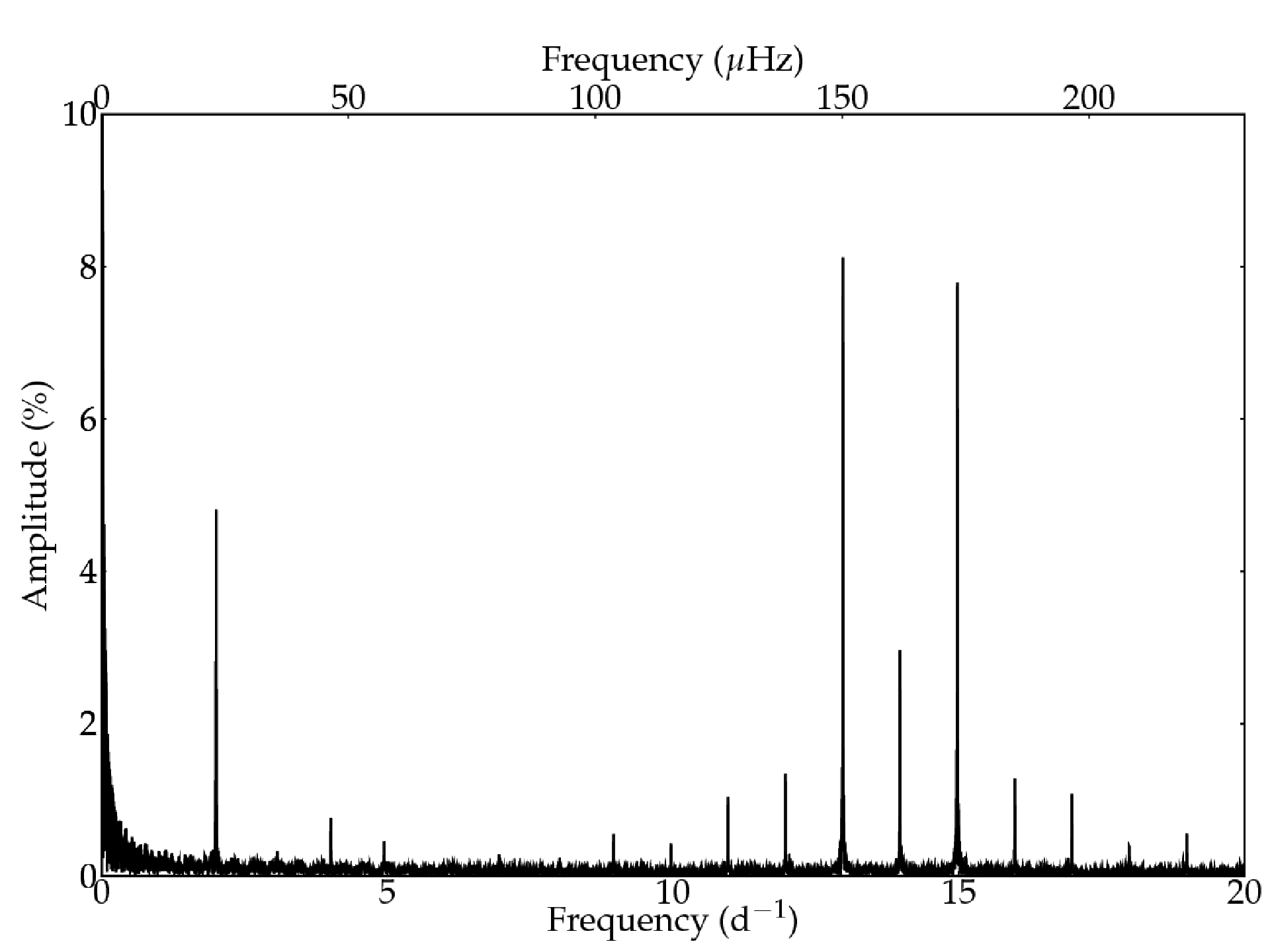
The raw light curve from the CoRoT database contains 422 949 datapoints, with an average time sampling of 32 s during 156.6 days and starting on . This brings the Nyquist frequency up to 1350 d-1. To obtain the highest possible precision, roughly of the datapoints were deleted because of flagged datapoints () and extreme outliers ( have an estimated error value above the level), keeping 379 785 datapoints (Fig. 1).
After rigorous tests, we decided not to interpolate the remaining points, because the improvements of the spectral window do not weigh up against the introduced uncertainties connected with the gap filling model. The highest amplitude in the window function is only of the main amplitude (Fig. 2). This means that we effectively spread out the power of each peak over several peaks, mainly well separated by d-1.
A raw estimate of the noise level of the light curve, computed as the average of the periodogram between 30 d-1 and 40 d-1 is at 57 mag or 0.00536 % in relative flux units, and slowly decays at higher frequencies to 24 mag or 0.0026 % between 100 d-1 and 110 d-1. We do not convert the light curve to magnitudes because the transformation from flux is not uniform and the theoretically predicted variations in first order are only linear in flux units. An exception is made in the case where the CoRoT light curve is used in combination with ground based observations. This does not pose a problem because of the dominant mode’s large amplitude.
The final reduced version of the light curve has also been corrected for long term trends: among an exponential, parabolic and linear trend, the linear trend resulted in the best fit, reducing significantly the power in the periodogram at low frequencies. An instrumental cause of the trend seems most probable, although long term (periodical) variations in the brightness of the star cannot be excluded from this time series alone. Previous ground based observations disfavour the second possibility, but do not exclude it, however.
2.2 The noise properties of the CoRoT data
The CoRoT data products contain information on the standard deviation of the star’s intensity per second, which is interpreted as the noise on the data. For the use and interpretation of the applied data analysis tools, it is vital to have a good understanding of the noise properties. We divided the error by the local average flux value of the light curve represented by a polynomial fit. A comparison between the Fourier periodogram of the intensity measurements and the derived standard deviations, shows that in the case of HD 180642, the latter are contaminated by the former, and are thus not a reliable estimate of the instrumental noise. Instead, we use the measurements of the constant star HD 181072 of spectral type A2 and visual magnitude of 9.14, which has been observed simultaneously on the same CCD, as an appropriate representation of the noise properties.
Traditionally, uncorrelated homoscedastic white Gaussian noise is assumed in frequency analyses of Cep stars. If the number of data points is large enough, this implies that the distribution of the normalised Fourier periodogram can be reasonably well approximated by an exponential distribution (Schwarzenberg-Czerny, 1998). In the following paragraphs, we show that none of the assumptions are strictly true, but the deviations are so small that the classical methods can still be applied provided that a correction for correlated data is used.
By binning the noise measurements in samples of 1000 points, we can see that the noise is not uncorrelated nor homoscedastic: we identify a continuously rising trend of percent d-1 and a small temporary bump around day 130 (Fig. 3). From a - plot of the Scargle periodogram, it is apparent that the noise is not white: at very low frequencies ( d-1) there is some power excess due to the correlation effect. However, white noise is a good enough approximation for d-1.
Drawing random samples of 1000 points, reveals that the noise is also not Gaussian: the sample mean is consistently higher than the sample median, suggesting that the noise has nonzero skewness. When falsifying samples of 1000 consecutive points for normality, by testing simultaneously for skewness and excess kurtosis, 65% of the samples are rejected at a acceptance level. Bootstrapping the same number of samples of 1000 points yield a rejection rate of 85%. A Gaussian fit to the noise histogram overestimates the average and the number of small outliers, and it consistently underestimates the number of large outliers (Fig. 3). The skewnormal distribution (Azzalini & Capitanio, 1999, e.g.,)
| (1) |
is more appropriate to describe the overall noise specifications. For the CoRoT data, we derive values of and for the location and scale parameters, and a value of , which determines the shape of the distribution ( means the distribution is normal, means the distribution is right-skewed). These values imply right-skewed, leptokurtic distributed noise, with a skewness and an excess kurtosis .

Next, we simulate the influence of skewnormality on the parameter and error estimation of a model
To do so, we generate three collections of light curves, each set containing at least 500 light curves with highly skewed noise (). To the first set of light curves, we add a high S/N monoperiodic sinusoidal signal (S/N), to the second set a low S/N monoperiodic sinusoidal signal (S/N), and to the third set a superposition of 200 sinusoids with S/N between 3 and 190 (which mimics the CoRoT data of HD 180642). To estimate , we use the peak frequency in the Scargle periodogram of each light curve. The other parameters are determined via ordinary linear regression. Subsequently, the distribution of each estimator is compared with the theoretical formulae, as described by Montgomery & O’Donoghue (1999) but additionally taking correlation effects into account (Schwarzenberg-Czerny, 2003), e.g. the error estimate on the frequency is
| (2) |
where is the standard deviation of the residuals. The effective number of observations is estimated by counting the average distance between sign changes in the residuals. From Table 1, we can see that there is no discrepancy between an estimator and the real input value in the case of a monoperiodic, high S/N signal, besides the fact that the ‘theoretical’ error estimates, such as Eq. (2), are rather conservative. For a multiperiodic signal with low S/N, the same pattern emerges except for the amplitudes: the estimator of the amplitude is slightly biased towards smaller values, but is still well within the error bars. The opposite bias is found in the signals with a low S/N value, but here an extra bias is introduced because peaks disappear in the noise for low amplitude values.
Finally, we analyze the influence of skewness on the Scargle periodogram in a qualitatively way using a large number of simulations of skew normally distributed noise with different parameters. We only find some additional noise at low frequencies, but this effect is only apparent for very high values. A set of heteroscedastic skew normal samples also introduces additional noise at low frequencies, but again, the degree of heteroscedasticity has to be unrealistically high compared to the case of the CoRoT data, to have a significant influence.
In conclusion, although the deviation from uncorrelated homoscedastic white Gaussian noise is significant for the CoRoT data, it is not dramatic: we are dealing with a slightly right-skewed, leptokurtic distribution. The above simulations suggest that a significant influence on parameter and error estimation is only noticable for high departures of normality. Moreover, as will become clear in the following sections, the noise level is inherently low compared to the analyzed signals, and we are conservative in our significance criteria: in the following, we adopt a value of in hypothesis testing, so that an order-of-magnitude estimate of is important, rather than a precise value. If at all, only the correlation effects are worth taking into account for our analysis; this is done with the method outlined in Schwarzenberg-Czerny (2003).
| Set | Type | Frequency | Amplitude | Phase | |||
|---|---|---|---|---|---|---|---|
| Monoperiodic High S/N | estimator | ||||||
| input | |||||||
| Monoperiodic Low S/N | estimator | ||||||
| input | |||||||
| Multiperiodic | estimator | ||||||
| input |
3 Modelling of the CoRoT light curve
Most of the calculations concerning stellar oscillations of Cep stars assume modes with small amplitudes, to be able to treat multiperiodicity as a linear superposition of multiple modes with infinite lifetime. Fitting simple sine functions, each with constant frequency, amplitude and phase through data represents the simplest first order deviations from a theoretical equilibrium state of the star. However, when the perturbations are not confined to the linear regime, higher order effects can only be modelled when different sines are combined and/or harmonics are allowed for, spreading the signature of a nonlinear effect in a Fourier periodogram over a wide range of frequencies.
Several physical origins of nonlinear effects in a light curve are plausible. These include a nonlinear response of the stellar flux, leading to a distortion of the light curve (Garrido & Rodriguez, 1996, e.g.), nonlinear mode coupling through resonant interaction between different modes (Dziembowski, 1982; Buchler et al., 1997, e.g.), excitation of strange-mode oscillations in highly nonadiabatic regimes (Saio et al., 1998; Glatzel, 1994, e.g.). etc. In particular, nonlinear resonant mode coupling can be distinguished from complicated beating among linear modes by checking the occurrence of frequency and/or phase locking, which is not expected for a superposition of linear modes. Nonlinear oscillation signatures may also include time-variable amplitudes or phases.
Given that we are dealing with the light curve of a large-amplitude Cep star, which is of unprecedented quality and quantity, it is not a priori clear if a linear superposition of mode frequencies is the best approach to treat the variability in the CoRoT light curve of HD 180642. Therefore, we first perform a traditional linear analysis of the light curve. Next, some nonlinear models are constructed and fitted to the data, as well as compared with the fit assuming linear mode frequencies. This comparison is done by means of statistical criteria taking into account the number of free parameters. We thus deduce the most likely physical interpretation of the variability of HD 180642 from the data point of view.
3.1 Superposition of linear modes
The first analysis of the CoRoT light curve of HD 180642 was done according to the traditional method, using the linear Scargle periodogram (Scargle, 1982) and consecutive prewhitening, translating to a well-known model of the form
| (3) |
for frequencies. Here, , and denote the amplitudes, frequencies and phases. The model was evaluated at every time of observation . At each prewhitening stage, all amplitudes, phases and the constant factor were refitted using the original light curve. This method implies a frequency resolution of the order of the Rayleigh limit d-1, making the frequency determination less precise when several frequencies are confined to a region of this width.
It is well known that nonlinear least squares fitting in the time domain while leaving the frequencies, amplitudes and phases free, can improve seriously the fit quality compared to the case where the frequency values are fixed to those resulting from the periodogram, but also that the success of such a procedure is largely dependent on the appropriate choice of good starting values, particularly when many frequencies are present. The starting values we adopted for the amplitudes and phases are those that resulted from ordinary least squares regression, while we fixed the frequencies from the Scargle periodogram.
It was immediately clear from the first few detected frequencies that the Scargle periodogram is not the optimal choice to describe or detect the variability of HD 180642, although it is most certainly a powerful indicator and intuitive. At least three harmonics of the main frequency were detected, with two more being marginally significant. Also the second independent frequency was best modeled with several harmonics (see upper right panel of Fig. 4). The amplitudes of the remaining frequencies are small enough to be modelled by single sines, as illustrated for four of them in Fig. 4. This figure also shows that the light curve cannot be adequately modelled by only a few frequencies and their harmonics.

The result of this traditional analysis is a wealth in frequencies, excluding clearly a monoperiodic model. We calculated up to 200 statistically significant frequencies (Table 7), although it has to be noted that “only” about 100 of them would be considered as not due to noise using the traditional signal-to-noise criterion of Breger et al. (1993). However, there is no doubt that the peaks are not due to noise because of two reasons. First, even after prewhitening 200 frequencies with a nonlinear least squares fit, the residual amplitudes are far above the instrumental noise level (discussed in Sect. 2.2), which would be expected if the signal would be composed of a superposition of linear modes. This can also be seen in Fig. 12, which we will discuss further in the text. Second, it is instructive to describe the distribution of frequencies across the spectrum, to see where all the frequencies reside. If most of the detected peaks are due to noise, they should be more or less randomly distributed across the analyzed frequency spectrum. In order to make the interpretation more clear, we decided to prewhiten a model of the first dominant mode and its five significant harmonics, or
| (4) |
where the initial harmonic fit was improved with a nonlinear least squares fit, letting also the frequency variable but with fixed harmonic combinations. Then, a power spectrum normalized by the total variance of the prewhitened data (denoted as ) was calculated. This means that the expected noise level under the assumption of Gaussian white noise corresponds to . The small deviation from this assumption (see Sect. 2.2), implies that slightly underestimates the true noise level. Next, the periodogram was averaged using Gaussian filters with d-1 (to smooth out the peaks) and d-1 to estimate the empirical noise level. The result is shown in Fig. 5. Noticeable power excess exists around d-1, d-1, d-1, d-1, d-1, d-1, d-1, d-1, d-1, d-1, d-1, and, finally, to a lesser extent also d-1. Most of these power excess regions are not due to one large peak, but represent a smoothing of many closely spaced peaks in the periodogram, e.g., in the low frequency region ( d-1). It is clear that the low amplitude frequencies are not due to noise, but is actual signal; it is apparent that there are almost no frequencies nor any sign of power excess in the region between d-1 and d-1. The higher frequency regions ( d-1) are much closer to the theoretical noise level, but are at the same time contaminated by secondary window peaks.

As it turned out, several of the frequencies are linear combinations of other frequencies (Table 2). The influence of a few frequencies is thus widely spread over the entire frequency spectrum. This is why we consider the second model discussed below.
3.2 Nonlinear frequency locking
Frequencies excited through nonlinear resonant mode coupling can manifest themselves in a natural way through combination frequencies, which may seem, at first sight, independent from the others. Such frequency locking is one effect that can be derived from the Amplitude Equation formalism (Dziembowski, 1982; Buchler et al., 1997; Van Hoolst et al., 1998, e.g.), if amplitudes and phases are constant in time. Following this assumption, a summary of the most obvious combination frequencies is given in Table 2. All combination frequencies were identified following the method described in Degroote et al. (2009). We selected only those combinations where the difference between the true combination value and the real value is below half of the Rayleigh limit d-1. The nonlinear leakage can then be viewed to spread over a wide range of the frequency spectrum, roughly between d-1 and d-1.
This phenomenon of combination frequencies has been detected previously in Cep stars, e.g. in Eri (Handler et al., 2004) and in 12 Lac (Handler et al., 2006). For these stars, only positive combinations were detected. It was difficult, therefore, to interpret these combinations, either in terms of light curve distortions due to nonlinear response or due to nonlinear resonant mode coupling. Indeed, both these phenomena would naturally give rise to difference combination frequencies as well as phase locking, which were not detected in these two stars. Moreover, third order combinations were not unambiguously identified, either because the amplitudes were too low, or they were not excited.
Under the assumption that the combination frequencies are real in HD 180642, the amplitudes, phases and independent frequencies were refitted using the previous values as starting values, while fixing the dependent frequencies according to their linear combination throughout the fit:
| (5) |
with
a linear combination of two independent frequencies. It is assumed that there are independent frequencies, and dependent frequencies.
In order to better describe the combination frequencies and their origin, their relative phases and amplitudes were analysed. Following Buchler et al. (1997) and Vuille (2000), they are defined as
and
with the subindex referring to the parent mode with the largest amplitude, to the parent mode with the smallest amplitude and the index to the daughter mode. The relative phases and amplitudes for all candidate combination frequencies, except harmonics, from Table 2 are shown in Fig. 6.
To make the discussion more readable, we denote each daughter mode by a unique designation,
where and are indices of the largest and smallest amplitude parent modes respectively (the higher this index, the lower the amplitude), and are the corresponding coefficients in the linear combinations (Table 2). Sum frequencies are distinguished from differences by the sign of the coefficients. Several interesting features appear:
- 1.
There are six daughter frequencies which have four properties in common: they are a sum of the dominant mode with another frequency, they cluster around the same relative phase (), they have comparable relative amplitudes and they have the same first-order coefficients (): , , , , and .
- 2.
A similar clustering around a common relative phase is visible for 6 differences: , , , , and , although they have different coefficients and different relative amplitudes.
- 3.
Around the second harmonic of the dominant mode, a spacing with d-1 is clearly visible. The daughter frequencies , have almost the same relative amplitudes, and are both found in two consecutive prewhitening stages.
- 4.
The daughter frequency has a relative phase of
The result for the fit using model is provided in Table 8 while a summary diagram of the independent and combination frequencies is shown in Fig. 7.


| ID | (d-1) | (d-1) | (d-1) | (d-1) | ||
|---|---|---|---|---|---|---|
| 1 | 5.48689 | 1 | 6.32482 | 11.81164 | 0.00006 | |
| -1 | 5.48689 | 1 | 6.32482 | 0.83794 | 0.00001 | |
| 2 | 5.48689 | 1 | 6.32482 | 17.29841 | 0.0002 | |
| 2 | 5.48689 | -1 | 6.32482 | 4.64845 | 0.0005 | |
| 1 | 5.48689 | 1 | 0.29917 | 5.78662 | 0.0006 | |
| 1 | 5.48689 | -1 | 0.29917 | 5.18781 | 0.00009 | |
| 2 | 5.48689 | -1 | 0.29917 | 10.67458 | 0.00002 | |
| 2 | 5.48689 | -2 | 0.29917 | 10.37493 | 0.0005 | |
| 1 | 5.48689 | -3 | 0.29917 | 4.58920 | 0.0002 | |
| 1 | 5.48689 | 1 | 8.40918 | 13.89585 | 0.0002 | |
| -1 | 5.48689 | 1 | 8.40918 | 2.92159 | 0.0007 | |
| 1 | 5.48689 | 1 | 6.14336 | 11.63039 | 0.0001 | |
| 1 | 5.48689 | 1 | 7.35867 | 12.84432 | 0.001 | |
| 1 | 5.48689 | 1 | 8.77086 | 14.25740 | 0.0003 | |
| 1 | 5.48689 | 1 | 6.26517 | 11.75173 | 0.0003 | |
| 1 | 7.25476 | -1 | 6.14336 | 1.11216 | 0.0008 | |
| 2 | 7.25476 | -1 | 6.14336 | 8.36870 | 0.0025 | |
| 1 | 8.40918 | -1 | 7.35866 | 1.04985 | 0.0007 | |
| 1 | 7.10353 | 3 | 0.89870 | 9.79999 | 0.0003 |
In the case of HD 180642, we hence do see difference combination frequencies, in contrast to the cases of the two large-amplitude Cep stars Eri (Handler et al., 2004) and 12 Lac (Handler et al., 2006). These difference frequencies are still well above 0.1 d-1, and are thus in the regime of white noise (see Fig.3) Such low combination frequencies are expected to occur with similar amplitudes as the sum combinations, for both the nonlinear distortion model and a nonlinear resonant mode coupling model. While we see more sum frequencies than differences, we do reach the regime of g-mode frequencies through several combinations for HD 180642. We also found higher order combinations here, up to order four (see Table 2), than for Eri and 12 Lac.
We note from Fig. 6 that four combination frequencies have a much higher -value than the others. This is simply due to the fact that these are the four combinations not involving the dominant mode (hence the denominator in the definition of is much smaller). Further, the relative amplitudes of the combinations involving the dominant mode cover a range of a factor ten and the phases cover the entire range , although several relative phases of difference frequencies are equal within the error bars, and similarly for the sum frequencies. The largest relative amplitudes all occur for a sum frequency due to a three-mode resonance model involving the dominant mode. The difference frequencies of the same three modes, if they occur, all have lower relative amplitude. We interpret this as due to nonlinear resonant mode locking, as a nonlinear distortion would not privilege larger amplitudes for sum or difference frequencies.
In principle, the relative amplitudes of the resonantly locked frequencies can help to constrain the mode degrees, because the geometric cancelling effect is different for different degrees. Unfortunately, we cannot use the relative amplitude values to derive the mode degrees, because all large-amplitude three mode resonances involve the dominant radial mode which does not imply geometric cancelling, and we have no other information on the degrees of the parent frequencies.
3.3 Time dependent amplitudes and phases
In the previous section, we assumed the amplitudes and phases to be constant in time. However, the Amplitude Equation formalism also allows for solutions where this is not the case (Buchler et al., 1997). Amplitude and phase modulations may occur, which can be (multi)periodic or chaotic. The light curve of HD 180642 as measured with CoRoT is of such high quality, that it becomes possible to detect and model these variations through changes in the highly sampled phase profile. Although a sine function with five harmonics is a good fit in the phase diagram (Fig. 4), it is also clear from the same figure that this model is only an ‘average’ model; in fact, the fit is not optimal to model a particular phase. Some phases can be modelled adequately with three harmonics, others need four, etc. Moreover, the minima and maxima seem to oscillate around an equilibrium value.
To quantify this time-dependent behaviour, a harmonic fit was calculated for every covered phase of the main frequency. The number of harmonics to be used is determined from the statistic of the data with respect to the model. The number of significant harmonics was taken as the lowest one that achieves a . This number varies mainly between three and four, with few exceptions.
We quantify the complexity of each phase profile by the ratio of the harmonic’s amplitudes compared to the main amplitude. The higher this ratio, the more significant the specific harmonic is. Also, from each fit, we extract the fitted constant as an indicator for long term trends. Finally, peak-to-peak variations in the phases are calculated. Using these methods, we finally arrive at an adapted version of Eq. (4):
| (6) |
with
For clarity, we first examine what the linear interpretation of this model would be. The simple model with and can be linearized with the assumption that . Violation of this assumption only influences the amplitude determination. Linearizing (6) gives
| (7) |
or when
| (8) |
with, under the assumption that ,
The results of the frequency analysis for the amplitudes, phases and constants for this model assumption can be found in Tables 9 to 16. The analysis of the first frequency of the time-dependent amplitude and phase for each harmonic is shown in Fig. 8.
With this last expansion in mind, we can use the results of the frequency analysis of the amplitudes and phases to predict the occurrence of spurious frequencies, actually originating from the linear expansion of the nonlinear model, and thus not physically inherent to the star. We performed this exercise for the primary component of the main radial mode and its harmonics. If we assume that the primary component and its harmonics have a variable amplitude and phase with frequency d-1, then we can already explain the occurrence of several of the observed frequencies (see Table 3). Obviously, not all predicted frequencies are discovered. After fitting the light curve with this model and inspecting the periodogram, we can see that there are additional secondary peaks introduced which are not observed. When taking more frequencies into account, at least some of the secondary peaks seem to cancel out. This motivated us to construct several time-dependent amplitude models and to compare the fits. From Tables 9 to 16, we selected the most probable frequencies and let the amplitudes and phases vary accordingly. First, we tried with only one frequency. Gradually we added more frequencies, until we arrived at a maximum of four frequencies determining the amplitude time variability.
The two frequencies 0.836 d-1 and 1.767 d-1 clearly stand out: the amplitudes and phases oscillate on this time scale, but they are also found when applying model given by Eq. (3), which means that the ‘entire’ light curve is also oscillating at the same rate. This is confirmed by analyzing the residuals after removing the constructed models: both of the frequencies are recovered.
Despite the success of these time-dependent amplitude and phase models to explain several peaks in the periodogram, we have to compare them more rigorously with the models of the forms Eqs (3) and (5), which is the topic of the next section.
| component | secondary | spurious frequency | Error |
|---|---|---|---|
| 0.8379 | 6.3248 | Observed | |
| -0.8379 | 4.6490 | Observed | |
| 0.8379 | 11.8168 | Observed | |
| -0.8379 | 10.1359 | - | |
| 0.8379 | 17.2986 | Observed | |
| -0.8379 | 10.1359 | - |
| component | secondary | spurious frequency | Error |
|---|---|---|---|
| 1.7678 | 7.2546 | Observed | |
| -1.7678 | 3.7191 | - | |
| 1.7678 | 12.7412 | Observed | |
| -1.7678 | 9.2060 | - | |
| 1.7678 | 18.2285 | - | |
| -1.7678 | 14.6928 | - |
| component | secondary | spurious frequency | Error |
|---|---|---|---|
| 2.5650 | 8.0519 | - | |
| -2.5650 | 2.9219 | Observed | |
| 2.5650 | 13.5388 | - | |
| -2.5650 | 8.4088 | Observed | |
| 2.5650 | 19.0257 | - | |
| -2.5650 | 13.8957 | Observed |


3.4 Model evaluation
To compare the different models with each other and determine their goodness-of-fit, we compute four evaluation statistics: the variance reduction (VR), both Akaike’s Information Criterion (AIC) and the Bayesian Information Criterion (BIC) in the time domain, and the power reduction (PR) in the frequency domain. The AIC is defined as
| (9) |
where is a maximum likelihood estimator (MLE), is the effective number of observations and is the number of free parameters in the model. Under the assumption of Gaussian white noise, we can insert the MLE of the noise variance, with RSS the residual sum of squares. Criterion (9) then becomes
The AIC can be calculated for every model, but is only relevant in comparisons; the lower the AIC, the better the model.
Despite the fact that the AIC discourages the use of too many free parameters (unlike the variance and power reduction), the BIC is more suited when we want to stress the importance of simpler models over more complicated ones and thus increase the penalty for introducing new parameters. The BIC is defined as
| (10) |
Analogous to the AIC, we can simplify this to
The BIC is also only relevant in comparisons, where again the lower the BIC, the better the model. We choose to use the BIC for our model selection rather than the criteria, because we want to favour simple physically appropriate models with the fewest possible degrees of freedom. The BIC is the most conservative criterion in this respect, because it requires that the gain in variance reduction must be worth the cost of introducing extra parameters.
First, we computed the AIC and BIC for all prewhitening stages. Indeed, given the richness of the frequency spectrum, it could well be that not all variability can be modeled adequately with sine functions. Of course any type of variability can be considered as such, but this may result in the use of too many parameters. As can be seen on Fig. 9, the BIC sets the optimal number of sines to use for model fit to 127; the introduction of 3 additional parameters is not worth the gain in variance reduction any longer.

From Table 4, we can see that all statistics prefer the model where the combination frequencies were fixed, except for the variance reduction. That the latter is slightly worse is no surprise, as the number of free parameters is much smaller with fixed frequencies.
All versions of the model described by Eq. (6) lead to a worse fit to the data than similar models (in the sense of which peaks they can explain) of the form of Eq. (3). The differences are small in most cases, but there is a difference nonetheless. This was already foreseen in Table 3 because not all predicted peaks are detectable, hence the fit introduces spurious peaks. This effect can also be deduced from the PR: although more parameters, the fits explain the periodogram less well than simpler models.
| Model | AIC (%) | BIC (%) | VR (%) | PR (%) | |
|---|---|---|---|---|---|
| Eq. (5), fixed comb | 94.010 | 94.065 | 97.755 | 25.50 | 78 |
| Eq. (3), Scargle freqs | 94.023 | 94.171 | 97.761 | 25.49 | 100 |
| Eq. (3), NLLS freqs | 94.021 | 94.169 | 97.762 | 25.49 | 100 |
| Eq. (6), 1 freq | 95.417 | 95.378 | 96.873 | 30.81 | 40 |
| Eq. (3), Scargle freqs | 95.405 | 95.314 | 96.872 | 30.87 | 28 |
| Eq. (3), NLLS freqs | 95.404 | 95.314 | 96.872 | 30.85 | 28 |
| Eq. (6), 2 freqs | 95.228 | 95.255 | 97.019 | 30.14 | 58 |
| Eq. (3), Scargle freqs | 95.204 | 95.130 | 97.017 | 30.24 | 34 |
| Eq. (3), NLLS freqs | 95.204 | 95.130 | 97.017 | 30.22 | 34 |
| Eq. (6), 3 freqs | 94.887 | 97.974 | 97.255 | 28.65 | 76 |
| Eq. (3), Scargle freqs | 94.837 | 94.783 | 97.263 | 28.84 | 43 |
| Eq. (3), NLLS freqs | 94.837 | 94.783 | 97.263 | 28.82 | 43 |
| Eq. (6), 4 freqs | 94.746 | 94.901 | 97.355 | 27.99 | 94 |
| Eq. (3), Scargle freqs | 94.687 | 94.664 | 97.361 | 28.29 | 52 |
| Eq. (3), NLLS freqs | 94.687 | 94.664 | 97.361 | 28.29 | 52 |
4 Time-frequency behaviour of parent and combination frequencies
The enormous complexity of the power spectrum of HD 180642 as measured with CoRoT and many of the previous remarks raise questions about the stability of the observed and treated modes in terms of amplitudes and frequencies. Nonlinear resonant mode coupling may give rise to variability in the frequencies and amplitudes over time (Buchler et al., 1997). Given that this is statistically the best model, and also physically the more plausible one, we focus on the modes listed in Table 2, by performing a time-frequency analysis for every prewhitening stage where the frequency under consideration is the dominant one.
A logical approach is to perform a wavelet analysis, adapted to the unequidistant signature of the dataset at hand (Foster, 1996). In a data set with a low enough noise level, one can also compare the shape of the detected peak in the Fourier periodogram with the theoretical shape of an infinitely stable mode of frequency :
with the total time span. This method has the advantage that we concentrate on the most localized area possible in frequency space. On the downside, a peak not fitting the expected shape can also mean that there is a beating pattern on a longer time scale which is not well resolved by the data sets. A third method to investigate stability we applied is simply to cut the entire time series in half, and do an independent traditional Scargle analysis on both parts.
The results for some of the frequencies in Table 2 are shown in Fig. 10, where the window for the wavelet transforms was taken as 40 days around the targeted frequencies. The dominant mode frequency and its first harmonic does not change during the entire CoRoT time series. Comparing the shapes of all the other peaks (some of which shown in the left panels of Fig. 10) leads to the conclusion that some frequencies do not change their behaviour while others do. This is particularly the case for d-1. The wavelet analysis hints towards changes in the amplitudes of many of the modes, but it does not allow thorough quantitative conclusions. Strong amplitude changes have also been found in the CoRoT data of the pulsating Be star HD 49330 (Huat et al., 2009).


5 Long term frequency evolution of the dominant mode
The Hipparcos satellite observed HD 180642 from March 12, 1990 during almost three years. Since then, 191 observations assembled with the photomultiplier P7 attached to the 0.7m Swiss telescope at La Silla and to the 1.2m Mercator telescope at La Palma were added. Moreover, we downloaded 310 archival ASAS data points (Pigulski & Pojmański, 2008). This brings the total time span of observations to 6814 days. The characteristics of the different datasets, as well as the first frequency value determined for each of these data sets are summarized in Table 5 and Fig. 11.

| (y) | (d) | (d-1) | (d-1) | (Hz) | ||
|---|---|---|---|---|---|---|
| Hipparcos | 1990 | 1091 | 83 | 5.4871 | 0.00006 | 63.508(2) |
| Swiss 70cm/P7 | 1997 | 187 | 20 | 5.4869 | 0.0002 | 63.50(5) |
| Mercator/P7 | 2002 | 1184 | 171 | 5.48693 | 0.00001 | 63.506(1) |
| ASAS | 2001 | 2798 | 310 | 5.48691 | 0.00001 | 63.505(9) |
| CoRoT/SISMO | 2007 | 156 | 379 785 | 5.48689 | 0.00003 | 63.505(7) |
| All | 1990 | 6814 | 380 369 | 5.48694 | 0.00003 | 63.506(3) |
The estimator (2) of the error on the frequency suggests that the precision simply scales with the total time span , which would hypothetically lower the frequency error by several magnitudes in our case if the datasets were to be combined. However, we have to take into account the extremely biased distribution of observations in time: more than of the observations are made during a time span only covering less than of the total time span. A natural measure for the uncertainty on the frequency is given by the width of the peak in the window function around . When adding only 83 datapoints to nearly half a million measurements, only tiny ‘wobbles’ are added to the window function and the overall shape of the main peaks is unaltered.
Instead of combining the datasets to model the stability of the frequency, we treat the datasets separately, and test if the frequency derived from Hipparcos measurements are equal to the one derived from the CoRoT mission, within estimated errors. In the CoRoT dataset correlation effects are taken into account. To determine how accurate the error estimation is in the case of the Hipparcos data, we randomly drew 7000 samples from the CoRoT dataset, using the (scaled) time gaps from the Hipparcos measurements, to arrive at a comparable number of datapoints () in each sample. We derive an empirical frequency error estimate of d-1, while formula (2) gives us a conservatively overestimated average value of d-1.
If the frequencies for the dominant mode from Hipparcos and CoRoT are estimates for a common mean , then the maximum likelihood estimator for is d-1, with a probability of . These facts suggest that the frequency of the dominant mode is not the same in these two data sets, but has instead decreased. From the datasets in Table 5, it is impossible to determine if the frequency change is gradual or sudden, so we refrain from any physical interpretation, although it would be naturally explained as a frequency decrease due to the approaching of the star to the end of the core-hydrogen burning, as suggested by the low of 3.45 dex.
6 Residual power
As already hinted at above when discussing the three models and , we did not yet reach the noise level when considering all the 127 frequencies listed in Table 7, or the more restricted lists belonging to models and given in Tables 15 to 16. Figure 12 shows the residual periodograms for each of the three considered models, where we took the time-variable amplitude and phase model allowing for one frequency to describe this amplitude variability as this leads to the best BIC (Table 4), but the result is similar for the other three cases of this model. As can be seen, all three models lead to residual power excess, although at a quite different level. Further prewhitening according to model was done (see Table 7 which lists up to 200 frequencies) but is, according to us, not very useful for a physical interpretation of the frequencies.


Recently, Belkacem et al. (2009) interpreted the residual power of HD 180642 after prewhitening 91 frequencies with a model description as , in terms of stochastically excited modes due to turbulent convection. They derived a large spacing Hz or twice this value, from the residual power spectrum, excluding the frequencies below 130Hz (11.23 d-1) and above 300Hz (26 d-1). We refer to their paper for a physical description and interpretation of such modes.
Our model comparison shows that the residual power is quite different for our preferred physical model than for model considering 127 frequencies. Even though model leads to lower residual power, it is statistically less good than model if one takes into account the difference in degrees of freedom. Also, ‘natural’ combination frequencies occur among the found frequencies, of which several are phase-locked. One may then wonder how frequencies which are resonantly excited and which may show time-dependent behaviour can be distinguished from stochastically excited ones, when they occur in the same frequency regime. In any case, the frequencies involved in phase locking are not expected to have a stochastic nature, as they would have random phase behaviour. Therefore, all the combination frequencies whose phases are locked (6 sum and 6 difference frequencies — see Fig. 6) are likely not due to a stochastic process. They cover almost the entire range in frequency covered in Fig. 7.
We estimated the large separations for the three residual power spectra shown in Fig. 12, assuming them to be caused by stochastically excited oscillations (p-modes), by using échelle diagrams with extracted frequencies and autocorrelations (Christensen-Dalsgaard, 1988). We thus find, in the frequency range from 50 Hz to 300 Hz, Hz for the residuals of model , Hz for the residuals of model and Hz for the residuals of model . The autocorrelation diagram for the residuals of the models also shows a smaller bump around 24 Hz and 36 Hz. Assuming modes as the cause of , could be interpreted as the distance between and modes but we regard this as a tentative result which needs further confirmation.
The detection of solar-like oscillations in this Cep star as an explanation of the residual excess power seems to be robust against the various models for the prewhitening of the -driven and resonantly excited modes. The value of the large spacing is, however, light curve model dependent.
7 Discussion and conclusion
The available CoRoT data of the Cep star HD 180642 provided us with a wealth of information.
Beyond the previously known dominant mode, many more frequencies are detected. A large fraction of those does not change their behaviour during the time span of the CoRoT data, while others do. Light curve modelling using different underlying functional assumptions led us to prefer a model based on nonlinear mode interaction, with 11 independent frequencies and 22 three-resonance combinations (among which some harmonics) covering the frequency range d-1. This model selection was based on statistical criteria, without considering physical arguments a priori. Nine of the independent frequencies of this model are in the range expected for Cep stars, i.e., between 5 and 9 d-1. This model is also the most logical one in terms of physical interpretation. Indeed, the nonlinear frequency locking is a natural consequence of the large amplitude of the dominant radial mode of the star. Five of these 33 frequencies are in the regime of high-order g modes with frequencies below 2 d-1 for stellar models appropriate for the star. The relative amplitudes of the coupling frequencies differ an order of magnitude and seem to point towards nonlinear resonant mode excitation and phase locking for several of these frequencies, particularly for those in the g-mode frequency regime.
Our observational results constitute a fruitful starting point for detailed seismic modelling of this star, particularly if some of the frequencies derived here could be identified. An extensive ground-based observing campaign has been organised with that goal and is discussed in Briquet et al. (2009). As indicated on Fig. 7, it leads to fully consistent frequency results with those found here, with 9 high-amplitude frequencies in common.
Acknowledgements.
The research leading to these results has received funding from the European Research Council under the European Community’s Seventh Framework Programme (FP7/2007–2013)/ERC grant agreement n∘227224 (PROSPERITY), as well as from the Research Council of K.U.Leuven grant agreement GOA/2008/04 and from the Belgian PRODEX Office under contract C90309: CoRoT Data Exploitation. This work was supported by the italian ESS project, contract ASI/INAF I/015/07/0, WP 03170. KU acknowledges financial support from a European Community Marie Curie Intra-European Fellowship, contract number MEIF-CT-2006-024476.References
- Aerts (2000) Aerts, C. 2000, A&A, 361, 245
- Auvergne et al. (2009) Auvergne, M., Bodin, P., Boisnard, L., et al. 2009, A&A, in press
- Azzalini & Capitanio (1999) Azzalini, A. & Capitanio, A. 1999, J.Roy.Statist.Soc, Series B, 61, 579
- Belkacem et al. (2009) Belkacem, K., Samadi, R., Goupil, M.-J., et al. 2009, Science, 324, 1540
- Breger et al. (1993) Breger, M., Stich, J., Garrido, R., et al. 1993, A&A, 271, 482
- Briquet et al. (2009) Briquet, M., Uytterhoeven, K., De Cat, P., & et al. 2009, A&A, in press
- Buchler et al. (1997) Buchler, J. R., Goupil, M.-J., & Hansen, C. J. 1997, A&A, 321, 159
- Christensen-Dalsgaard (1988) Christensen-Dalsgaard, J. 1988, in IAU Symposium, Vol. 123, Advances in Helio- and Asteroseismology, ed. J. Christensen-Dalsgaard & S. Frandsen, 3
- Degroote et al. (2009) Degroote, P., Aerts, C., Baudin, F., et al. 2009, A&A, in press
- Dziembowski (1982) Dziembowski, W. 1982, Acta Astronomica, 32, 147
- Foster (1996) Foster, G. 1996, AJ, 112, 1709
- Fridlund et al. (2006) Fridlund, M., Baglin, A., Lochard, J., & Conroy, L., eds. 2006, ESA Special Publication, Vol. 1306, The CoRoT Mission Pre-Launch Status - Stellar Seismology and Planet Finding
- Garrido & Rodriguez (1996) Garrido, R. & Rodriguez, E. 1996, MNRAS, 281, 696
- Glatzel (1994) Glatzel, W. 1994, MNRAS, 271, 66
- Handler et al. (2006) Handler, G., Jerzykiewicz, M., Rodríguez, E., et al. 2006, MNRAS, 365, 327
- Handler et al. (2004) Handler, G., Shobbrook, R. R., Jerzykiewicz, M., et al. 2004, MNRAS, 347, 454
- Huat et al. (2009) Huat, A.-L., Hubert, A.-M., Floquet, M., et al. 2009, A&A, in press
- Montgomery & O’Donoghue (1999) Montgomery, M. H. & O’Donoghue, D. 1999, Delta Scuti Star Newsletter, 13, 28
- Morel & Aerts (2007) Morel, T. & Aerts, C. 2007, Communications in Asteroseismology, 150, 201
- Morel et al. (2006) Morel, T., Butler, K., Aerts, C., Neiner, C., & Briquet, M. 2006, A&A, 457, 651
- Morel et al. (2008) Morel, T., Hubrig, S., & Briquet, M. 2008, A&A, 481, 453
- Pigulski & Pojmański (2008) Pigulski, A. & Pojmański, G. 2008, A&A, 477, 907
- Saio et al. (1998) Saio, H., Baker, N. H., & Gautschy, A. 1998, MNRAS, 294, 622
- Scargle (1982) Scargle, J. D. 1982, ApJ, 263, 835
- Schwarzenberg-Czerny (1996) Schwarzenberg-Czerny, A. 1996, ApJ, 460, L107
- Schwarzenberg-Czerny (1998) Schwarzenberg-Czerny, A. 1998, MNRAS, 301, 831
- Schwarzenberg-Czerny (2003) Schwarzenberg-Czerny, A. 2003, in Astronomical Society of the Pacific Conference Series, Vol. 292, Interplay of Periodic, Cyclic and Stochastic Variability in Selected Areas of the H-R Diagram, ed. C. Sterken, 383
- Stankov & Handler (2005) Stankov, A. & Handler, G. 2005, ApJS, 158, 193
- Uytterhoeven et al. (2008) Uytterhoeven, K., Poretti, E., Rainer, M., et al. 2008, Journal of Physics Conference Series, 118, 012077
- Van Hoolst et al. (1998) Van Hoolst, T., Dziembowski, W. A., & Kawaler, S. D. 1998, MNRAS, 297, 536
- Vuille (2000) Vuille, F. 2000, Baltic Astronomy, 9, 33
- Waelkens et al. (1998) Waelkens, C., Aerts, C., Kestens, E., Grenon, M., & Eyer, L. 1998, A&A, 330, 215
Appendix A Frequency tables
| (d-1) | (d-1) | (Hz) | (Hz) | SNR | VR | AIC | BIC | |||||
|---|---|---|---|---|---|---|---|---|---|---|---|---|
| 1 | 5.486889 | 0.000023 | 63.505662 | 0.000262 | 0.03696 | 0.00024 | -0.0355 | 0.0064 | 188.7 | 91.86 | 100.00 | 100.00 |
| 2 | 10.973740 | 0.000062 | 127.010883 | 0.000721 | 0.00631 | 0.00011 | -0.4938 | 0.0177 | 63.0 | 94.54 | 98.24 | 98.18 |
| 3 | 16.460665 | 0.000080 | 190.516954 | 0.000928 | 0.00405 | 0.00009 | 0.3492 | 0.0227 | 70.4 | 95.65 | 97.25 | 97.15 |
| 4 | 0.299171 | 0.000093 | 3.462623 | 0.001073 | 0.00313 | 0.00008 | -0.3748 | 0.0263 | 27.8 | 96.31 | 96.53 | 96.41 |
| 5 | 6.324816 | 0.000120 | 73.203886 | 0.001389 | 0.00224 | 0.00008 | -0.2335 | 0.0340 | 21.8 | 96.64 | 96.11 | 95.98 |
| 6 | 8.409185 | 0.000161 | 97.328527 | 0.001864 | 0.00156 | 0.00007 | 0.4594 | 0.0457 | 17.9 | 96.81 | 95.89 | 95.77 |
| 7 | 7.254757 | 0.000162 | 83.967094 | 0.001875 | 0.00145 | 0.00007 | -0.0600 | 0.0460 | 16.5 | 96.95 | 95.70 | 95.58 |
| 8 | 21.947560 | 0.000184 | 254.022686 | 0.002130 | 0.00127 | 0.00007 | 0.1164 | 0.0522 | 36.6 | 97.06 | 95.54 | 95.42 |
| 9 | 11.811640 | 0.000193 | 136.708796 | 0.002232 | 0.00119 | 0.00007 | -0.4081 | 0.0547 | 15.4 | 97.16 | 95.40 | 95.29 |
| 10 | 6.143358 | 0.000233 | 71.103681 | 0.002696 | 0.00100 | 0.00007 | -0.0105 | 0.0661 | 10.1 | 97.22 | 95.30 | 95.19 |
| 11 | 7.103534 | 0.000224 | 82.216823 | 0.002595 | 0.00100 | 0.00006 | 0.3475 | 0.0636 | 11.5 | 97.29 | 95.19 | 95.10 |
| 12 | 1.112160 | 0.000234 | 12.872226 | 0.002710 | 0.00095 | 0.00006 | -0.1078 | 0.0664 | 9.4 | 97.35 | 95.09 | 95.01 |
| 13 | 13.895848 | 0.000235 | 160.831579 | 0.002716 | 0.00094 | 0.00006 | 0.2959 | 0.0666 | 14.9 | 97.41 | 95.00 | 94.92 |
| 14 | 1.024105 | 0.000240 | 11.853066 | 0.002775 | 0.00089 | 0.00006 | -0.4860 | 0.0680 | 8.9 | 97.46 | 94.91 | 94.84 |
| 15 | 7.358664 | 0.000248 | 85.169719 | 0.002874 | 0.00085 | 0.00006 | 0.3891 | 0.0705 | 10.2 | 97.51 | 94.83 | 94.77 |
| 16 | 1.049850 | 0.000240 | 12.151046 | 0.002779 | 0.00084 | 0.00006 | 0.2368 | 0.0681 | 8.6 | 97.56 | 94.75 | 94.69 |
| 17 | 0.898703 | 0.000246 | 10.401656 | 0.002843 | 0.00084 | 0.00006 | 0.1240 | 0.0697 | 8.5 | 97.61 | 94.66 | 94.62 |
| 18 | 7.245672 | 0.000233 | 83.861941 | 0.002697 | 0.00085 | 0.00006 | 0.1250 | 0.0661 | 9.7 | 97.65 | 94.58 | 94.55 |
| 19 | 0.741254 | 0.000280 | 8.579333 | 0.003243 | 0.00071 | 0.00006 | -0.4799 | 0.0795 | 7.2 | 97.69 | 94.52 | 94.50 |
| 20 | 0.320416 | 0.000287 | 3.708515 | 0.003325 | 0.00067 | 0.00005 | -0.4893 | 0.0815 | 6.6 | 97.72 | 94.47 | 94.45 |
| 21 | 7.374444 | 0.000287 | 85.352356 | 0.003321 | 0.00066 | 0.00005 | -0.3128 | 0.0814 | 7.9 | 97.74 | 94.42 | 94.41 |
| 22 | 11.630388 | 0.000287 | 134.610967 | 0.003326 | 0.00065 | 0.00005 | -0.1838 | 0.0815 | 8.9 | 97.77 | 94.37 | 94.37 |
| 23 | 0.837937 | 0.000290 | 9.698339 | 0.003362 | 0.00064 | 0.00005 | -0.4509 | 0.0824 | 6.7 | 97.80 | 94.31 | 94.33 |
| 24 | 0.573389 | 0.000304 | 6.636450 | 0.003514 | 0.00061 | 0.00005 | 0.0670 | 0.0861 | 6.3 | 97.83 | 94.27 | 94.29 |
| 25 | 0.613211 | 0.000297 | 7.097346 | 0.003440 | 0.00062 | 0.00005 | 0.3570 | 0.0843 | 6.5 | 97.85 | 94.22 | 94.25 |
| 26 | 0.437363 | 0.000304 | 5.062076 | 0.003515 | 0.00060 | 0.00005 | -0.2705 | 0.0862 | 6.2 | 97.88 | 94.17 | 94.22 |
| 27 | 0.387200 | 0.000306 | 4.481479 | 0.003547 | 0.00059 | 0.00005 | 0.3086 | 0.0869 | 6.1 | 97.90 | 94.13 | 94.18 |
| 28 | 2.921596 | 0.000304 | 33.814774 | 0.003514 | 0.00058 | 0.00005 | -0.4474 | 0.0861 | 6.0 | 97.92 | 94.08 | 94.15 |
| 29 | 10.361777 | 0.000302 | 119.927974 | 0.003496 | 0.00058 | 0.00005 | -0.3554 | 0.0857 | 7.7 | 97.94 | 94.04 | 94.12 |
| 30 | 0.100806 | 0.000308 | 1.166736 | 0.003565 | 0.00058 | 0.00005 | -0.0958 | 0.0874 | 6.1 | 97.97 | 93.99 | 94.08 |
| 31 | 8.396265 | 0.000307 | 97.178990 | 0.003548 | 0.00057 | 0.00005 | 0.2305 | 0.0870 | 7.3 | 97.99 | 93.95 | 94.05 |
| 32 | 1.205832 | 0.000308 | 13.956386 | 0.003563 | 0.00056 | 0.00005 | -0.4130 | 0.0873 | 6.1 | 98.01 | 93.91 | 94.02 |
| 33 | 0.285145 | 0.000320 | 3.300292 | 0.003706 | 0.00055 | 0.00005 | -0.2305 | 0.0908 | 5.8 | 98.03 | 93.87 | 93.99 |
| 34 | 8.770865 | 0.000326 | 101.514639 | 0.003768 | 0.00053 | 0.00005 | -0.0214 | 0.0924 | 6.9 | 98.05 | 93.83 | 93.96 |
| 35 | 0.335229 | 0.000323 | 3.879971 | 0.003743 | 0.00053 | 0.00005 | 0.4316 | 0.0917 | 5.6 | 98.07 | 93.79 | 93.93 |
| 36 | 0.257337 | 0.000327 | 2.978433 | 0.003783 | 0.00052 | 0.00005 | -0.2497 | 0.0927 | 5.6 | 98.08 | 93.75 | 93.91 |
| 37 | 0.009469 | 0.000310 | 0.109600 | 0.003582 | 0.00055 | 0.00005 | -0.0817 | 0.0878 | 5.6 | 98.10 | 93.72 | 93.88 |
| 38 | 0.370980 | 0.000332 | 4.293751 | 0.003840 | 0.00050 | 0.00005 | -0.0996 | 0.0941 | 5.3 | 98.12 | 93.68 | 93.86 |
| 39 | 7.425424 | 0.000350 | 85.942402 | 0.004053 | 0.00047 | 0.00005 | 0.0174 | 0.0994 | 5.9 | 98.13 | 93.65 | 93.84 |
| 40 | 5.684955 | 0.000351 | 65.798086 | 0.004058 | 0.00047 | 0.00005 | -0.1344 | 0.0995 | 5.3 | 98.15 | 93.62 | 93.82 |
| 41 | 0.187774 | 0.000349 | 2.173308 | 0.004043 | 0.00047 | 0.00005 | -0.2518 | 0.0991 | 5.2 | 98.16 | 93.59 | 93.80 |
| 42 | 7.191284 | 0.000355 | 83.232453 | 0.004109 | 0.00046 | 0.00005 | 0.3525 | 0.1007 | 5.8 | 98.18 | 93.56 | 93.78 |
| 43 | 8.331328 | 0.000356 | 96.427411 | 0.004123 | 0.00046 | 0.00005 | -0.4133 | 0.1011 | 6.0 | 98.19 | 93.53 | 93.76 |
| 44 | 0.091000 | 0.000354 | 1.053236 | 0.004102 | 0.00046 | 0.00005 | -0.1169 | 0.1005 | 4.9 | 98.20 | 93.50 | 93.74 |
| 45 | 0.050942 | 0.000364 | 0.589602 | 0.004213 | 0.00044 | 0.00005 | 0.4170 | 0.1033 | 4.9 | 98.22 | 93.47 | 93.72 |
| 46 | 0.026107 | 0.000356 | 0.302160 | 0.004124 | 0.00045 | 0.00005 | -0.4822 | 0.1011 | 4.9 | 98.23 | 93.44 | 93.71 |
| 47 | 5.187812 | 0.000373 | 60.044119 | 0.004317 | 0.00043 | 0.00005 | 0.4664 | 0.1058 | 4.9 | 98.24 | 93.42 | 93.69 |
| 48 | 10.674584 | 0.000369 | 123.548429 | 0.004270 | 0.00043 | 0.00004 | -0.2976 | 0.1047 | 5.9 | 98.25 | 93.39 | 93.67 |
| 49 | 10.374926 | 0.000379 | 120.080167 | 0.004382 | 0.00042 | 0.00004 | -0.2046 | 0.1074 | 5.7 | 98.26 | 93.36 | 93.66 |
| 50 | 7.109275 | 0.000377 | 82.283274 | 0.004361 | 0.00042 | 0.00004 | 0.0798 | 0.1069 | 5.2 | 98.28 | 93.34 | 93.65 |
| 51 | 8.368705 | 0.000372 | 96.860009 | 0.004309 | 0.00042 | 0.00004 | -0.0134 | 0.1056 | 5.5 | 98.29 | 93.31 | 93.63 |
| 52 | 0.476009 | 0.000373 | 5.509363 | 0.004319 | 0.00042 | 0.00004 | -0.3027 | 0.1059 | 4.8 | 98.30 | 93.28 | 93.62 |
| 53 | 1.122346 | 0.000370 | 12.990121 | 0.004288 | 0.00041 | 0.00004 | 0.1337 | 0.1051 | 4.7 | 98.31 | 93.26 | 93.60 |
| 54 | 6.265172 | 0.000393 | 72.513563 | 0.004549 | 0.00039 | 0.00004 | 0.0353 | 0.1115 | 4.7 | 98.32 | 93.23 | 93.59 |
| 55 | 17.298406 | 0.000393 | 200.213032 | 0.004550 | 0.00039 | 0.00004 | 0.3315 | 0.1115 | 9.1 | 98.33 | 93.21 | 93.58 |
| 56 | 0.130294 | 0.000397 | 1.508027 | 0.004589 | 0.00039 | 0.00004 | -0.1917 | 0.1125 | 4.5 | 98.34 | 93.19 | 93.57 |
| 57 | 7.323153 | 0.000399 | 84.758713 | 0.004618 | 0.00038 | 0.00004 | -0.0064 | 0.1132 | 5.0 | 98.35 | 93.16 | 93.56 |
| 58 | 7.064826 | 0.000402 | 81.768818 | 0.004648 | 0.00038 | 0.00004 | -0.4697 | 0.1139 | 4.8 | 98.36 | 93.14 | 93.54 |
| 59 | 7.177056 | 0.000398 | 83.067776 | 0.004602 | 0.00038 | 0.00004 | 0.4879 | 0.1128 | 4.9 | 98.37 | 93.12 | 93.53 |
| 60 | 0.419303 | 0.000398 | 4.853043 | 0.004602 | 0.00038 | 0.00004 | 0.4717 | 0.1128 | 4.4 | 98.38 | 93.10 | 93.52 |
| 61 | 8.266944 | 0.000408 | 95.682225 | 0.004721 | 0.00037 | 0.00004 | -0.1626 | 0.1157 | 5.0 | 98.39 | 93.08 | 93.51 |
| 62 | 0.068790 | 0.000393 | 0.796186 | 0.004548 | 0.00038 | 0.00004 | 0.2876 | 0.1115 | 4.3 | 98.40 | 93.05 | 93.50 |
| 63 | 0.598913 | 0.000400 | 6.931862 | 0.004624 | 0.00037 | 0.00004 | 0.2735 | 0.1133 | 4.4 | 98.41 | 93.03 | 93.49 |
| 64 | 4.648449 | 0.000410 | 53.801491 | 0.004747 | 0.00036 | 0.00004 | 0.2154 | 0.1163 | 4.2 | 98.42 | 93.01 | 93.48 |
| 65 | 1.062249 | 0.000405 | 12.294552 | 0.004689 | 0.00036 | 0.00004 | -0.1036 | 0.1149 | 4.4 | 98.42 | 92.99 | 93.47 |
| 66 | 7.530514 | 0.000407 | 87.158725 | 0.004716 | 0.00036 | 0.00004 | 0.1886 | 0.1156 | 4.8 | 98.43 | 92.97 | 93.46 |
| 67 | 8.851947 | 0.000408 | 102.453088 | 0.004720 | 0.00036 | 0.00004 | 0.4543 | 0.1157 | 5.0 | 98.44 | 92.95 | 93.46 |
| 68 | 0.200097 | 0.000404 | 2.315934 | 0.004679 | 0.00036 | 0.00004 | 0.4588 | 0.1147 | 4.3 | 98.45 | 92.93 | 93.45 |
| 69 | 7.804933 | 0.000410 | 90.334876 | 0.004746 | 0.00035 | 0.00004 | 0.3967 | 0.1163 | 4.8 | 98.46 | 92.91 | 93.44 |
| 70 | 7.451400 | 0.000405 | 86.243060 | 0.004688 | 0.00035 | 0.00004 | 0.1652 | 0.1149 | 4.7 | 98.47 | 92.89 | 93.43 |
| 71 | 10.399457 | 0.000410 | 120.364087 | 0.004749 | 0.00035 | 0.00004 | 0.1639 | 0.1164 | 5.0 | 98.48 | 92.87 | 93.42 |
| 72 | 1.045241 | 0.000364 | 12.097692 | 0.004209 | 0.00039 | 0.00004 | -0.1921 | 0.1032 | 4.2 | 98.48 | 92.85 | 93.41 |
| 73 | 11.573429 | 0.000417 | 133.951724 | 0.004829 | 0.00034 | 0.00004 | 0.2994 | 0.1184 | 5.1 | 98.49 | 92.83 | 93.41 |
| 74 | 8.779805 | 0.000400 | 101.618112 | 0.004630 | 0.00035 | 0.00004 | -0.4466 | 0.1135 | 4.8 | 98.50 | 92.81 | 93.40 |
| 75 | 7.498775 | 0.000416 | 86.791379 | 0.004815 | 0.00034 | 0.00004 | 0.4624 | 0.1180 | 4.6 | 98.51 | 92.79 | 93.39 |
| 76 | 9.799902 | 0.000419 | 113.424788 | 0.004851 | 0.00034 | 0.00004 | 0.0974 | 0.1189 | 4.9 | 98.51 | 92.77 | 93.39 |
| 77 | 8.763891 | 0.000409 | 101.433921 | 0.004738 | 0.00034 | 0.00004 | 0.2360 | 0.1161 | 4.8 | 98.52 | 92.75 | 93.38 |
| 78 | 1.618521 | 0.000412 | 18.732877 | 0.004765 | 0.00033 | 0.00004 | 0.1506 | 0.1168 | 4.1 | 98.53 | 92.74 | 93.37 |
| 79 | 8.872841 | 0.000417 | 102.694924 | 0.004824 | 0.00033 | 0.00004 | 0.0555 | 0.1182 | 4.7 | 98.54 | 92.72 | 93.36 |
| 80 | 0.176488 | 0.000411 | 2.042685 | 0.004754 | 0.00033 | 0.00004 | -0.0624 | 0.1165 | 4.0 | 98.54 | 92.70 | 93.36 |
| 81 | 1.935029 | 0.000424 | 22.396164 | 0.004910 | 0.00032 | 0.00004 | 0.0156 | 0.1203 | 4.0 | 98.55 | 92.68 | 93.35 |
| 82 | 0.380644 | 0.000404 | 4.405601 | 0.004673 | 0.00033 | 0.00004 | -0.3600 | 0.1145 | 3.9 | 98.56 | 92.66 | 93.35 |
| 83 | 7.417077 | 0.000408 | 85.845797 | 0.004719 | 0.00033 | 0.00004 | 0.3142 | 0.1157 | 4.4 | 98.56 | 92.65 | 93.34 |
| 84 | 1.520179 | 0.000427 | 17.594661 | 0.004939 | 0.00032 | 0.00004 | -0.4267 | 0.1211 | 3.9 | 98.57 | 92.63 | 93.33 |
| 85 | 0.222217 | 0.000422 | 2.571956 | 0.004887 | 0.00032 | 0.00004 | 0.4562 | 0.1198 | 3.9 | 98.58 | 92.61 | 93.33 |
| 86 | 8.359820 | 0.000410 | 96.757173 | 0.004747 | 0.00033 | 0.00004 | 0.4324 | 0.1164 | 4.5 | 98.58 | 92.60 | 93.32 |
| 87 | 7.259464 | 0.000385 | 84.021572 | 0.004457 | 0.00035 | 0.00004 | -0.1884 | 0.1092 | 4.3 | 98.59 | 92.58 | 93.32 |
| 88 | 7.380371 | 0.000419 | 85.420960 | 0.004849 | 0.00032 | 0.00004 | -0.0678 | 0.1188 | 4.3 | 98.60 | 92.56 | 93.31 |
| 89 | 7.479556 | 0.000421 | 86.568930 | 0.004873 | 0.00032 | 0.00004 | 0.2767 | 0.1194 | 4.4 | 98.60 | 92.54 | 93.31 |
| 90 | 4.874065 | 0.000442 | 56.412785 | 0.005113 | 0.00030 | 0.00004 | -0.3730 | 0.1253 | 3.8 | 98.61 | 92.53 | 93.30 |
| 91 | 8.688025 | 0.000442 | 100.555841 | 0.005119 | 0.00030 | 0.00004 | -0.3248 | 0.1255 | 4.4 | 98.62 | 92.51 | 93.30 |
| 92 | 5.609340 | 0.000434 | 64.922921 | 0.005029 | 0.00030 | 0.00004 | 0.2954 | 0.1233 | 3.9 | 98.62 | 92.50 | 93.30 |
| 93 | 9.825918 | 0.000436 | 113.725898 | 0.005042 | 0.00030 | 0.00004 | -0.1101 | 0.1236 | 4.5 | 98.63 | 92.48 | 93.29 |
| 94 | 0.430350 | 0.000426 | 4.980899 | 0.004934 | 0.00031 | 0.00004 | -0.1086 | 0.1209 | 3.7 | 98.63 | 92.46 | 93.29 |
| 95 | 1.070228 | 0.000420 | 12.386895 | 0.004862 | 0.00031 | 0.00004 | -0.4757 | 0.1192 | 3.9 | 98.64 | 92.45 | 93.28 |
| 96 | 5.786624 | 0.000435 | 66.974815 | 0.005032 | 0.00030 | 0.00004 | 0.2157 | 0.1233 | 3.9 | 98.65 | 92.43 | 93.28 |
| 97 | 6.031242 | 0.000438 | 69.806041 | 0.005066 | 0.00030 | 0.00004 | 0.4529 | 0.1242 | 3.9 | 98.65 | 92.42 | 93.28 |
| 98 | 7.123896 | 0.000428 | 82.452503 | 0.004953 | 0.00030 | 0.00004 | -0.3384 | 0.1214 | 4.1 | 98.66 | 92.40 | 93.27 |
| 99 | 13.818031 | 0.000443 | 159.930915 | 0.005129 | 0.00029 | 0.00004 | 0.3384 | 0.1257 | 5.2 | 98.66 | 92.39 | 93.27 |
| 100 | 0.038176 | 0.000434 | 0.441848 | 0.005022 | 0.00030 | 0.00004 | 0.3760 | 0.1231 | 3.8 | 98.67 | 92.37 | 93.27 |
| 101 | 0.409477 | 0.000407 | 4.739314 | 0.004708 | 0.00031 | 0.00004 | -0.2513 | 0.1154 | 3.7 | 98.67 | 92.36 | 93.26 |
| 102 | 1.411052 | 0.000436 | 16.331623 | 0.005050 | 0.00029 | 0.00004 | 0.2190 | 0.1238 | 3.8 | 98.68 | 92.34 | 93.26 |
| 103 | 0.521680 | 0.000439 | 6.037968 | 0.005078 | 0.00029 | 0.00004 | -0.3007 | 0.1245 | 3.8 | 98.69 | 92.33 | 93.25 |
| 104 | 7.221801 | 0.000436 | 83.585665 | 0.005043 | 0.00029 | 0.00004 | 0.2655 | 0.1236 | 4.1 | 98.69 | 92.31 | 93.25 |
| 105 | 0.114405 | 0.000440 | 1.324132 | 0.005092 | 0.00029 | 0.00004 | 0.0372 | 0.1248 | 3.7 | 98.70 | 92.30 | 93.25 |
| 106 | 0.228917 | 0.000444 | 2.649499 | 0.005136 | 0.00029 | 0.00004 | -0.2926 | 0.1259 | 3.7 | 98.70 | 92.28 | 93.25 |
| 107 | 7.466602 | 0.000443 | 86.419001 | 0.005127 | 0.00029 | 0.00004 | -0.1099 | 0.1257 | 4.0 | 98.71 | 92.27 | 93.24 |
| 108 | 13.291190 | 0.000452 | 153.833214 | 0.005236 | 0.00028 | 0.00004 | 0.3146 | 0.1283 | 4.9 | 98.71 | 92.25 | 93.24 |
| 109 | 8.807314 | 0.000449 | 101.936500 | 0.005200 | 0.00028 | 0.00004 | -0.4451 | 0.1274 | 4.2 | 98.72 | 92.24 | 93.24 |
| 110 | 8.823592 | 0.000412 | 102.124902 | 0.004772 | 0.00031 | 0.00004 | -0.3130 | 0.1170 | 4.5 | 98.72 | 92.22 | 93.23 |
| 111 | 8.837597 | 0.000434 | 102.287004 | 0.005019 | 0.00029 | 0.00004 | -0.0539 | 0.1230 | 4.3 | 98.73 | 92.21 | 93.23 |
| 112 | 6.362414 | 0.000444 | 73.639052 | 0.005137 | 0.00028 | 0.00003 | -0.1784 | 0.1259 | 3.8 | 98.73 | 92.19 | 93.23 |
| 113 | 8.302855 | 0.000444 | 96.097863 | 0.005135 | 0.00028 | 0.00003 | -0.4654 | 0.1259 | 4.1 | 98.74 | 92.18 | 93.23 |
| 114 | 9.868206 | 0.000447 | 114.215342 | 0.005174 | 0.00027 | 0.00003 | -0.4197 | 0.1268 | 4.2 | 98.74 | 92.16 | 93.22 |
| 115 | 19.382612 | 0.000449 | 224.335786 | 0.005202 | 0.00027 | 0.00003 | 0.0761 | 0.1275 | 7.5 | 98.75 | 92.15 | 93.22 |
| 116 | 8.735203 | 0.000451 | 101.101887 | 0.005221 | 0.00027 | 0.00003 | 0.0035 | 0.1280 | 4.1 | 98.75 | 92.14 | 93.22 |
| 117 | 0.137406 | 0.000446 | 1.590343 | 0.005163 | 0.00027 | 0.00003 | 0.2740 | 0.1266 | 3.5 | 98.76 | 92.12 | 93.22 |
| 118 | 8.376218 | 0.000444 | 96.946966 | 0.005136 | 0.00027 | 0.00003 | 0.1986 | 0.1259 | 4.0 | 98.76 | 92.11 | 93.22 |
| 119 | 1.143357 | 0.000460 | 13.233304 | 0.005327 | 0.00027 | 0.00003 | -0.0138 | 0.1306 | 3.6 | 98.77 | 92.10 | 93.22 |
| 120 | 10.449163 | 0.000467 | 120.939385 | 0.005406 | 0.00026 | 0.00003 | 0.4923 | 0.1325 | 4.1 | 98.77 | 92.08 | 93.22 |
| 121 | 7.184473 | 0.000455 | 83.153622 | 0.005271 | 0.00027 | 0.00003 | 0.1653 | 0.1292 | 3.8 | 98.78 | 92.07 | 93.22 |
| 122 | 12.588851 | 0.000468 | 145.704299 | 0.005418 | 0.00026 | 0.00003 | 0.0927 | 0.1328 | 4.5 | 98.78 | 92.06 | 93.21 |
| 123 | 1.347183 | 0.000473 | 15.592394 | 0.005479 | 0.00026 | 0.00003 | 0.3051 | 0.1343 | 3.5 | 98.79 | 92.05 | 93.21 |
| 124 | 4.375634 | 0.000474 | 50.643915 | 0.005483 | 0.00026 | 0.00003 | -0.2058 | 0.1344 | 3.5 | 98.79 | 92.03 | 93.21 |
| 125 | 15.849010 | 0.000472 | 183.437619 | 0.005461 | 0.00026 | 0.00003 | 0.4390 | 0.1339 | 5.7 | 98.79 | 92.02 | 93.21 |
| 126 | 0.542048 | 0.000473 | 6.273707 | 0.005470 | 0.00025 | 0.00003 | -0.3701 | 0.1341 | 3.4 | 98.80 | 92.01 | 93.21 |
| 127 | 0.989224 | 0.000468 | 11.449349 | 0.005411 | 0.00025 | 0.00003 | 0.4361 | 0.1326 | 3.5 | 98.80 | 92.00 | 93.21 |
| 128 | 4.463677 | 0.000470 | 51.662926 | 0.005437 | 0.00025 | 0.00003 | 0.1705 | 0.1333 | 3.4 | 98.81 | 91.98 | 93.21 |
| 129 | 1.457477 | 0.000474 | 16.868952 | 0.005483 | 0.00025 | 0.00003 | -0.2285 | 0.1344 | 3.4 | 98.81 | 91.97 | 93.21 |
| 130 | 0.270580 | 0.000468 | 3.131714 | 0.005412 | 0.00025 | 0.00003 | -0.1148 | 0.1327 | 3.3 | 98.82 | 91.96 | 93.21 |
| 131 | 7.917871 | 0.000482 | 91.642025 | 0.005580 | 0.00025 | 0.00003 | -0.2305 | 0.1368 | 3.7 | 98.82 | 91.95 | 93.21 |
| 132 | 1.296026 | 0.000483 | 15.000305 | 0.005589 | 0.00025 | 0.00003 | -0.4679 | 0.1370 | 3.4 | 98.82 | 91.94 | 93.22 |
| 133 | 0.237799 | 0.000454 | 2.752299 | 0.005256 | 0.00026 | 0.00003 | -0.3142 | 0.1288 | 3.3 | 98.83 | 91.93 | 93.22 |
| 134 | 2.043672 | 0.000478 | 23.653608 | 0.005535 | 0.00025 | 0.00003 | -0.0814 | 0.1357 | 3.5 | 98.83 | 91.92 | 93.22 |
| 135 | 0.736254 | 0.000447 | 8.521458 | 0.005169 | 0.00026 | 0.00003 | 0.1303 | 0.1267 | 3.4 | 98.84 | 91.90 | 93.22 |
| 136 | 0.924792 | 0.000474 | 10.703616 | 0.005483 | 0.00024 | 0.00003 | 0.3061 | 0.1344 | 3.4 | 98.84 | 91.89 | 93.22 |
| 137 | 6.274253 | 0.000455 | 72.618664 | 0.005271 | 0.00025 | 0.00003 | -0.0798 | 0.1292 | 3.5 | 98.84 | 91.88 | 93.22 |
| 138 | 0.453644 | 0.000455 | 5.250507 | 0.005268 | 0.00025 | 0.00003 | 0.1580 | 0.1291 | 3.4 | 98.85 | 91.87 | 93.22 |
| 139 | 8.352350 | 0.000463 | 96.670712 | 0.005356 | 0.00025 | 0.00003 | 0.2023 | 0.1313 | 3.7 | 98.85 | 91.86 | 93.22 |
| 140 | 1.128681 | 0.000462 | 13.063439 | 0.005343 | 0.00025 | 0.00003 | 0.4418 | 0.1310 | 3.4 | 98.86 | 91.85 | 93.22 |
| 141 | 2.157032 | 0.000474 | 24.965648 | 0.005490 | 0.00024 | 0.00003 | 0.4815 | 0.1346 | 3.5 | 98.86 | 91.83 | 93.22 |
| 142 | 14.257403 | 0.000477 | 165.016241 | 0.005526 | 0.00024 | 0.00003 | -0.1181 | 0.1355 | 4.6 | 98.86 | 91.82 | 93.22 |
| 143 | 1.038144 | 0.000470 | 12.015553 | 0.005439 | 0.00024 | 0.00003 | -0.2466 | 0.1333 | 3.4 | 98.87 | 91.81 | 93.22 |
| 144 | 2.427459 | 0.000484 | 28.095586 | 0.005598 | 0.00023 | 0.00003 | -0.1941 | 0.1372 | 3.4 | 98.87 | 91.80 | 93.22 |
| 145 | 0.347300 | 0.000475 | 4.019673 | 0.005495 | 0.00024 | 0.00003 | -0.2060 | 0.1347 | 3.3 | 98.87 | 91.79 | 93.22 |
| 146 | 11.751733 | 0.000487 | 136.015424 | 0.005638 | 0.00023 | 0.00003 | -0.1587 | 0.1382 | 4.0 | 98.88 | 91.78 | 93.23 |
| 147 | 7.278539 | 0.000482 | 84.242348 | 0.005576 | 0.00024 | 0.00003 | -0.4180 | 0.1367 | 3.5 | 98.88 | 91.77 | 93.23 |
| 148 | 7.333070 | 0.000459 | 84.873501 | 0.005313 | 0.00025 | 0.00003 | -0.1156 | 0.1302 | 3.5 | 98.88 | 91.76 | 93.23 |
| 149 | 12.955309 | 0.000487 | 149.945711 | 0.005633 | 0.00023 | 0.00003 | 0.4954 | 0.1381 | 4.2 | 98.89 | 91.75 | 93.23 |
| 150 | 12.844315 | 0.000487 | 148.661057 | 0.005641 | 0.00023 | 0.00003 | 0.1819 | 0.1383 | 4.2 | 98.89 | 91.74 | 93.23 |
| 151 | 6.201708 | 0.000483 | 71.779026 | 0.005588 | 0.00023 | 0.00003 | -0.2326 | 0.1370 | 3.4 | 98.90 | 91.73 | 93.23 |
| 152 | 4.437075 | 0.000481 | 51.355038 | 0.005565 | 0.00023 | 0.00003 | 0.4883 | 0.1364 | 3.3 | 98.90 | 91.72 | 93.23 |
| 153 | 0.674955 | 0.000478 | 7.811985 | 0.005533 | 0.00023 | 0.00003 | 0.1507 | 0.1356 | 3.3 | 98.90 | 91.70 | 93.23 |
| 154 | 7.295163 | 0.000468 | 84.434760 | 0.005421 | 0.00024 | 0.00003 | -0.1483 | 0.1329 | 3.5 | 98.91 | 91.69 | 93.24 |
| 155 | 8.289375 | 0.000476 | 95.941836 | 0.005509 | 0.00023 | 0.00003 | -0.4974 | 0.1350 | 3.6 | 98.91 | 91.68 | 93.24 |
| 156 | 13.790030 | 0.000479 | 159.606828 | 0.005547 | 0.00023 | 0.00003 | 0.3534 | 0.1360 | 4.3 | 98.91 | 91.67 | 93.24 |
| 157 | 2.790366 | 0.000486 | 32.295906 | 0.005625 | 0.00023 | 0.00003 | -0.3009 | 0.1379 | 3.3 | 98.92 | 91.66 | 93.24 |
| 158 | 6.330152 | 0.000466 | 73.265645 | 0.005390 | 0.00023 | 0.00003 | 0.0448 | 0.1321 | 3.3 | 98.92 | 91.65 | 93.24 |
| 159 | 11.546618 | 0.000482 | 133.641409 | 0.005580 | 0.00023 | 0.00003 | 0.1608 | 0.1368 | 3.9 | 98.92 | 91.64 | 93.24 |
| 160 | 10.219603 | 0.000484 | 118.282442 | 0.005602 | 0.00022 | 0.00003 | -0.1732 | 0.1373 | 3.7 | 98.93 | 91.63 | 93.25 |
| 161 | 8.168456 | 0.000483 | 94.542314 | 0.005595 | 0.00022 | 0.00003 | 0.4513 | 0.1371 | 3.6 | 98.93 | 91.62 | 93.25 |
| 162 | 0.658442 | 0.000479 | 7.620860 | 0.005549 | 0.00023 | 0.00003 | -0.2895 | 0.1360 | 3.2 | 98.93 | 91.61 | 93.25 |
| 163 | 16.161520 | 0.000492 | 187.054627 | 0.005696 | 0.00022 | 0.00003 | 0.4617 | 0.1396 | 5.3 | 98.94 | 91.60 | 93.25 |
| 164 | 7.442907 | 0.000462 | 86.144753 | 0.005352 | 0.00023 | 0.00003 | -0.0362 | 0.1312 | 3.4 | 98.94 | 91.59 | 93.25 |
| 165 | 11.426610 | 0.000493 | 132.252429 | 0.005705 | 0.00022 | 0.00003 | 0.1803 | 0.1398 | 3.8 | 98.94 | 91.58 | 93.26 |
| 166 | 1.587122 | 0.000487 | 18.369468 | 0.005632 | 0.00022 | 0.00003 | 0.4358 | 0.1381 | 3.3 | 98.95 | 91.57 | 93.26 |
| 167 | 1.767490 | 0.000488 | 20.457055 | 0.005645 | 0.00022 | 0.00003 | -0.2663 | 0.1384 | 3.3 | 98.95 | 91.56 | 93.26 |
| 168 | 1.666735 | 0.000489 | 19.290919 | 0.005656 | 0.00022 | 0.00003 | -0.4967 | 0.1386 | 3.3 | 98.95 | 91.55 | 93.26 |
| 169 | 13.883301 | 0.000486 | 160.686356 | 0.005626 | 0.00022 | 0.00003 | -0.0029 | 0.1379 | 4.2 | 98.96 | 91.54 | 93.26 |
| 170 | 10.390805 | 0.000456 | 120.263944 | 0.005273 | 0.00023 | 0.00003 | 0.3919 | 0.1292 | 3.7 | 98.96 | 91.53 | 93.27 |
| 171 | 12.741223 | 0.000485 | 147.467860 | 0.005615 | 0.00022 | 0.00003 | -0.2775 | 0.1376 | 4.0 | 98.96 | 91.52 | 93.27 |
| 172 | 0.309166 | 0.000453 | 3.578306 | 0.005237 | 0.00023 | 0.00003 | 0.0626 | 0.1284 | 3.2 | 98.97 | 91.51 | 93.27 |
| 173 | 4.745479 | 0.000489 | 54.924531 | 0.005663 | 0.00022 | 0.00003 | 0.3323 | 0.1388 | 3.2 | 98.97 | 91.50 | 93.27 |
| 174 | 11.692495 | 0.000486 | 135.329801 | 0.005627 | 0.00022 | 0.00003 | -0.0403 | 0.1379 | 3.8 | 98.97 | 91.49 | 93.27 |
| 175 | 1.359556 | 0.000488 | 15.735597 | 0.005650 | 0.00022 | 0.00003 | 0.4042 | 0.1385 | 3.3 | 98.97 | 91.48 | 93.28 |
| 176 | 0.975971 | 0.000488 | 11.295957 | 0.005645 | 0.00022 | 0.00003 | -0.4811 | 0.1384 | 3.2 | 98.98 | 91.47 | 93.28 |
| 177 | 8.418358 | 0.000461 | 97.434701 | 0.005331 | 0.00023 | 0.00003 | -0.2797 | 0.1307 | 3.5 | 98.98 | 91.46 | 93.28 |
| 178 | 9.786730 | 0.000488 | 113.272343 | 0.005650 | 0.00021 | 0.00003 | -0.1297 | 0.1385 | 3.6 | 98.98 | 91.45 | 93.28 |
| 179 | 1.375485 | 0.000476 | 15.919966 | 0.005515 | 0.00022 | 0.00003 | 0.4005 | 0.1352 | 3.2 | 98.99 | 91.44 | 93.29 |
| 180 | 1.177101 | 0.000482 | 13.623856 | 0.005584 | 0.00021 | 0.00003 | -0.2543 | 0.1369 | 3.2 | 98.99 | 91.43 | 93.29 |
| 181 | 5.267010 | 0.000497 | 60.960760 | 0.005752 | 0.00021 | 0.00003 | -0.2691 | 0.1410 | 3.2 | 98.99 | 91.42 | 93.29 |
| 182 | 0.326968 | 0.000468 | 3.784349 | 0.005418 | 0.00022 | 0.00003 | 0.0205 | 0.1328 | 3.1 | 99.00 | 91.41 | 93.29 |
| 183 | 6.898981 | 0.000499 | 79.849312 | 0.005781 | 0.00021 | 0.00003 | 0.4291 | 0.1417 | 3.3 | 99.00 | 91.40 | 93.30 |
| 184 | 8.457694 | 0.000494 | 97.889973 | 0.005717 | 0.00021 | 0.00003 | -0.3974 | 0.1401 | 3.4 | 99.00 | 91.39 | 93.30 |
| 185 | 10.319399 | 0.000499 | 119.437493 | 0.005773 | 0.00021 | 0.00003 | 0.3013 | 0.1415 | 3.5 | 99.00 | 91.38 | 93.30 |
| 186 | 9.755457 | 0.000500 | 112.910384 | 0.005792 | 0.00021 | 0.00003 | -0.0400 | 0.1420 | 3.5 | 99.01 | 91.38 | 93.30 |
| 187 | 4.589204 | 0.000504 | 53.115787 | 0.005829 | 0.00021 | 0.00003 | -0.3857 | 0.1429 | 3.1 | 99.01 | 91.37 | 93.31 |
| 188 | 6.132605 | 0.000488 | 70.979230 | 0.005648 | 0.00021 | 0.00003 | -0.3332 | 0.1384 | 3.2 | 99.01 | 91.36 | 93.31 |
| 189 | 9.860127 | 0.000485 | 114.121844 | 0.005615 | 0.00021 | 0.00003 | -0.0811 | 0.1376 | 3.5 | 99.02 | 91.35 | 93.31 |
| 190 | 9.924674 | 0.000499 | 114.868909 | 0.005773 | 0.00020 | 0.00003 | 0.4594 | 0.1415 | 3.5 | 99.02 | 91.34 | 93.32 |
| 191 | 1.029558 | 0.000447 | 11.916180 | 0.005176 | 0.00023 | 0.00003 | -0.2873 | 0.1269 | 3.1 | 99.02 | 91.33 | 93.32 |
| 192 | 5.751525 | 0.000499 | 66.568575 | 0.005781 | 0.00020 | 0.00003 | 0.3417 | 0.1417 | 3.1 | 99.02 | 91.32 | 93.32 |
| 193 | 0.123769 | 0.000475 | 1.432511 | 0.005500 | 0.00022 | 0.00003 | 0.2788 | 0.1348 | 3.0 | 99.03 | 91.31 | 93.33 |
| 194 | 15.287241 | 0.000512 | 176.935655 | 0.005925 | 0.00020 | 0.00003 | -0.1422 | 0.1452 | 4.5 | 99.03 | 91.31 | 93.33 |
| 195 | 7.389585 | 0.000473 | 85.527608 | 0.005471 | 0.00021 | 0.00003 | 0.2971 | 0.1341 | 3.2 | 99.03 | 91.30 | 93.34 |
| 196 | 11.619288 | 0.000500 | 134.482497 | 0.005789 | 0.00020 | 0.00003 | 0.4728 | 0.1419 | 3.6 | 99.03 | 91.29 | 93.34 |
| 197 | 6.229125 | 0.000508 | 72.096349 | 0.005883 | 0.00020 | 0.00003 | 0.0977 | 0.1442 | 3.1 | 99.04 | 91.28 | 93.34 |
| 198 | 7.351882 | 0.000499 | 85.091228 | 0.005776 | 0.00020 | 0.00003 | 0.2438 | 0.1416 | 3.2 | 99.04 | 91.27 | 93.35 |
| 199 | 7.285282 | 0.000476 | 84.320395 | 0.005512 | 0.00021 | 0.00003 | -0.1116 | 0.1351 | 3.2 | 99.04 | 91.26 | 93.35 |
| 200 | 2.227274 | 0.000506 | 25.778639 | 0.005852 | 0.00020 | 0.00003 | -0.2862 | 0.1434 | 3.1 | 99.05 | 91.25 | 93.35 |
| (d-1) | (Hz) | SNR | VR | AIC | BIC | ||||||
|---|---|---|---|---|---|---|---|---|---|---|---|
| 0.036966 | 5.486888 | 63.50565 | -0.0355 | - | - | - | - | 188.7 | 91.86 | 100.00 | 100.01 |
| 0.006313 | 10.973776 | 127.01130 | -0.4967 | - | - | - | - | 63.0 | 94.54 | 98.25 | 98.20 |
| 0.004049 | 16.460665 | 190.51695 | 0.3490 | - | - | - | - | 70.4 | 95.64 | 97.26 | 97.18 |
| 0.003125 | 0.299178 | 3.46271 | -0.3753 | - | - | - | - | 27.8 | 96.31 | 96.54 | 96.45 |
| 0.002220 | 6.324787 | 73.20355 | -0.2322 | - | - | - | - | 21.8 | 96.64 | 96.12 | 96.04 |
| 0.001568 | 8.408990 | 97.32628 | 0.4746 | - | - | - | - | 17.9 | 96.81 | 95.91 | 95.83 |
| 0.001441 | 7.255010 | 83.97002 | -0.0764 | - | - | - | - | 16.5 | 96.95 | 95.72 | 95.65 |
| 0.001269 | 21.947553 | 254.02260 | 0.1169 | - | - | - | - | 36.6 | 97.06 | 95.56 | 95.51 |
| 0.001181 | 11.811675 | 136.70920 | -0.4118 | -4.82 | 0.01 | -0.14 | 0.01 | 15.4 | 97.15 | 95.42 | 95.36 |
| 0.001003 | 6.143123 | 71.10096 | 0.0079 | - | - | - | - | 10.1 | 97.22 | 95.32 | 95.28 |
| 0.000999 | 7.103595 | 82.21753 | 0.3435 | - | - | - | - | 11.5 | 97.29 | 95.21 | 95.19 |
| 0.000924 | 1.111887 | 12.86906 | -0.0844 | -3.17 | 0.02 | -0.06 | 0.02 | 9.4 | 97.35 | 95.11 | 95.09 |
| 0.000936 | 13.895879 | 160.83193 | 0.2930 | -4.76 | 0.02 | -0.12 | 0.01 | 14.9 | 97.41 | 95.01 | 94.98 |
| 0.000852 | 7.358900 | 85.17245 | 0.3698 | - | - | - | - | 10.2 | 97.46 | 94.94 | 94.92 |
| 0.000848 | 1.050091 | 12.15383 | 0.2169 | -3.17 | 0.02 | 0.17 | 0.02 | 8.6 | 97.50 | 94.85 | 94.84 |
| 0.000826 | 0.898758 | 10.40229 | 0.1134 | - | - | - | - | 8.5 | 97.55 | 94.78 | 94.77 |
| 0.000644 | 11.630011 | 134.60661 | -0.1515 | -4.74 | 0.02 | -0.14 | 0.02 | 8.9 | 97.58 | 94.72 | 94.72 |
| 0.000653 | 0.837898 | 9.69790 | -0.4485 | -5.07 | 0.02 | -0.25 | 0.02 | 6.7 | 97.61 | 94.67 | 94.67 |
| 0.000579 | 2.922102 | 33.82063 | -0.4912 | -4.98 | 0.02 | 0.06 | 0.02 | 6.0 | 97.63 | 94.63 | 94.62 |
| 0.000529 | 8.770800 | 101.51388 | -0.0181 | - | - | - | - | 6.9 | 97.65 | 94.60 | 94.61 |
| 0.000448 | 5.187710 | 60.04294 | 0.4809 | -5.39 | 0.02 | 0.13 | 0.02 | 4.9 | 97.66 | 94.58 | 94.59 |
| 0.000426 | 10.674598 | 123.54859 | -0.2978 | -5.41 | 0.03 | 0.40 | 0.02 | 5.9 | 97.68 | 94.55 | 94.56 |
| 0.000424 | 10.375420 | 120.08588 | -0.2473 | -5.41 | 0.03 | 0.12 | 0.02 | 5.7 | 97.69 | 94.53 | 94.54 |
| 0.000345 | 8.366896 | 96.83908 | 0.1436 | -3.60 | 0.04 | 0.10 | 0.03 | 5.5 | 97.70 | 94.51 | 94.52 |
| 0.000390 | 6.265160 | 72.51343 | 0.0363 | - | - | - | - | 4.7 | 97.71 | 94.50 | 94.53 |
| 0.000393 | 17.298563 | 200.21485 | 0.3194 | -5.30 | 0.03 | -0.36 | 0.02 | 9.1 | 97.72 | 94.48 | 94.51 |
| 0.000363 | 4.648990 | 53.80775 | 0.1698 | -5.33 | 0.03 | 0.05 | 0.02 | 4.2 | 97.73 | 94.46 | 94.49 |
| 0.000339 | 9.799869 | 113.42441 | 0.1004 | -3.36 | 0.04 | 0.38 | 0.04 | 4.9 | 97.73 | 94.45 | 94.47 |
| 0.000289 | 5.786066 | 66.96836 | 0.2604 | -5.58 | 0.03 | -0.37 | 0.02 | 3.9 | 97.74 | 94.44 | 94.46 |
| 0.000226 | 14.257688 | 165.01953 | -0.1453 | -4.91 | 0.04 | -0.06 | 0.03 | 4.6 | 97.74 | 94.43 | 94.45 |
| 0.000234 | 11.752049 | 136.01908 | -0.1853 | -4.77 | 0.05 | -0.16 | 0.03 | 4.0 | 97.75 | 94.42 | 94.45 |
| 0.000205 | 12.845788 | 148.67810 | 0.0760 | -5.16 | 0.04 | -0.17 | 0.03 | 4.2 | 97.75 | 94.42 | 94.44 |
| 0.000206 | 4.589353 | 53.11751 | -0.3901 | -5.72 | 0.04 | -0.47 | 0.03 | 3.1 | 97.75 | 94.41 | 94.44 |
| (d-1) | (Hz) | |||||
|---|---|---|---|---|---|---|
| 0.00244 | 0.00011 | 0.8379 | 0.0002 | 9.6985 | 0.13 | 0.05 |
| 0.00117 | 0.00011 | 1.7679 | 0.0003 | 20.4613 | 0.41 | 0.10 |
| 0.00087 | 0.00011 | 0.6564 | 0.0004 | 7.5976 | 0.34 | 0.10 |
| 0.00075 | 0.00011 | 1.7588 | 0.0005 | 20.3564 | -0.39 | 0.10 |
| 0.00066 | 0.00011 | 1.6160 | 0.0006 | 18.7031 | -0.18 | 0.20 |
| 0.00064 | 0.00011 | 0.2999 | 0.0006 | 3.4708 | -0.45 | 0.20 |
| 0.00062 | 0.00010 | 1.8717 | 0.0006 | 21.6636 | -0.17 | 0.20 |
| 0.00051 | 0.00010 | 1.8870 | 0.0007 | 21.8400 | 0.23 | 0.20 |
| 0.00046 | 0.00010 | 0.1976 | 0.0007 | 2.2865 | 0.21 | 0.20 |
| 0.00045 | 0.00010 | 1.9380 | 0.0007 | 22.4302 | -0.41 | 0.20 |
| (d-1) | (Hz) | |||||
|---|---|---|---|---|---|---|
| 0.00131 | 0.00011 | 2.5651 | 0.0003 | 29.6883 | 0.42 | 0.08 |
| 0.00085 | 0.00010 | 0.8377 | 0.0004 | 9.6958 | 0.34 | 0.10 |
| 0.00075 | 0.00010 | 1.7678 | 0.0005 | 20.4611 | 0.37 | 0.10 |
| 0.00061 | 0.00010 | 1.6166 | 0.0005 | 18.7106 | -0.19 | 0.20 |
| 0.00055 | 0.00010 | 0.5992 | 0.0006 | 6.9349 | 0.04 | 0.20 |
| 0.00047 | 0.00010 | 1.8708 | 0.0007 | 21.6530 | -0.06 | 0.20 |
| 0.00046 | 0.00008 | 0.6130 | 0.0007 | 7.0951 | 0.14 | 0.20 |
| 0.00045 | 0.00008 | 2.6428 | 0.0007 | 30.5880 | 0.34 | 0.20 |
| 0.00045 | 0.00008 | 0.2991 | 0.0007 | 3.4612 | 0.03 | 0.20 |
| 0.00043 | 0.00008 | 0.6561 | 0.0007 | 7.5937 | -0.44 | 0.20 |
| (d-1) | (Hz) | |||||
|---|---|---|---|---|---|---|
| 0.00087 | 0.00006 | 2.5650 | 0.0002 | 29.6870 | 0.46 | 0.07 |
| 0.00049 | 0.00005 | 0.8376 | 0.0004 | 9.6942 | 0.22 | 0.10 |
| 0.00027 | 0.00005 | 0.5993 | 0.0007 | 6.9367 | -0.02 | 0.20 |
| 0.00026 | 0.00005 | 2.6425 | 0.0007 | 30.5840 | 0.42 | 0.20 |
| 0.00026 | 0.00005 | 0.6569 | 0.0008 | 7.6031 | 0.34 | 0.20 |
| 0.00026 | 0.00005 | 1.7681 | 0.0007 | 20.4638 | 0.37 | 0.20 |
| 0.00024 | 0.00005 | 0.6126 | 0.0008 | 7.0899 | 0.16 | 0.20 |
| 0.00024 | 0.00005 | 2.2028 | 0.0008 | 25.4959 | -0.12 | 0.20 |
| 0.00023 | 0.00005 | 2.3188 | 0.0008 | 26.8375 | -0.07 | 0.20 |
| 0.00023 | 0.00005 | 0.2985 | 0.0008 | 3.4552 | 0.14 | 0.20 |
| (d-1) | (Hz) | |||||
|---|---|---|---|---|---|---|
| 0.00016 | 0.00004 | 0.8375 | 0.0008 | 9.6938 | -0.45 | 0.20 |
| (d-1) | (Hz) | |||||
|---|---|---|---|---|---|---|
| 0.00835 | 0.00050 | 0.8378 | 0.0002 | 9.6968 | -0.13 | 0.07 |
| 0.00539 | 0.00050 | 1.7679 | 0.0003 | 20.4616 | 0.12 | 0.10 |
| 0.00482 | 0.00050 | 0.6564 | 0.0004 | 7.5976 | 0.07 | 0.10 |
| 0.00436 | 0.00050 | 2.5644 | 0.0004 | 29.6802 | -0.15 | 0.10 |
| 0.00374 | 0.00040 | 1.6165 | 0.0004 | 18.7092 | -0.48 | 0.10 |
| 0.00344 | 0.00040 | 1.8718 | 0.0004 | 21.6646 | -0.44 | 0.10 |
| 0.00306 | 0.00040 | 1.7588 | 0.0005 | 20.3563 | 0.30 | 0.10 |
| 0.00234 | 0.00040 | 1.8876 | 0.0006 | 21.8470 | -0.11 | 0.20 |
| 0.00200 | 0.00040 | 0.7411 | 0.0007 | 8.5776 | 0.24 | 0.20 |
| 0.00197 | 0.00040 | 0.1982 | 0.0007 | 2.2940 | -0.08 | 0.20 |
| (d-1) | (Hz) | |||||
|---|---|---|---|---|---|---|
| 0.02791 | 0.00300 | 0.8380 | 0.0004 | 9.6994 | 0.11 | 0.10 |
| 0.02607 | 0.00300 | 2.5646 | 0.0004 | 29.6829 | -0.34 | 0.10 |
| 0.02034 | 0.00300 | 0.6572 | 0.0005 | 7.6063 | 0.33 | 0.10 |
| 0.01615 | 0.00300 | 0.6111 | 0.0006 | 7.0729 | 0.43 | 0.20 |
| 0.01317 | 0.00300 | 1.7676 | 0.0007 | 20.4588 | 0.20 | 0.20 |
| 0.01133 | 0.00300 | 0.2992 | 0.0008 | 3.4624 | 0.29 | 0.20 |
| 0.01123 | 0.00200 | 1.8724 | 0.0008 | 21.6711 | -0.40 | 0.20 |
| 0.01044 | 0.00200 | 1.1135 | 0.0008 | 12.8875 | 0.18 | 0.20 |
| 0.01073 | 0.00200 | 1.7594 | 0.0008 | 20.3632 | 0.31 | 0.20 |
| 0.01022 | 0.00200 | 0.5977 | 0.0008 | 6.9179 | 0.19 | 0.20 |
| (d-1) | (Hz) | |||||
|---|---|---|---|---|---|---|
| 0.03866 | 0.00300 | 2.5646 | 0.0003 | 29.6825 | -0.33 | 0.08 |
| 0.02706 | 0.00300 | 0.8379 | 0.0004 | 9.6982 | -0.01 | 0.10 |
| 0.01324 | 0.00300 | 0.6571 | 0.0008 | 7.6055 | 0.25 | 0.20 |
| 0.01300 | 0.00300 | 1.7679 | 0.0008 | 20.4618 | 0.28 | 0.20 |
| 0.01270 | 0.00300 | 1.9803 | 0.0008 | 22.9200 | 0.17 | 0.20 |
| 0.01199 | 0.00300 | 0.6095 | 0.0008 | 7.0547 | 0.50 | 0.20 |
| 0.01183 | 0.00300 | 2.0427 | 0.0008 | 23.6424 | -0.41 | 0.20 |
| 0.01106 | 0.00300 | 2.5777 | 0.0009 | 29.8348 | -0.05 | 0.30 |
| 0.01101 | 0.00300 | 1.1718 | 0.0009 | 13.5625 | 0.16 | 0.30 |
| 0.01049 | 0.00300 | 2.1939 | 0.0009 | 25.3920 | -0.49 | 0.30 |
| (d-1) | (Hz) | |||||
|---|---|---|---|---|---|---|
| 0.05623 | 0.00800 | 0.8378 | 0.0005 | 9.6970 | 0.16 | 0.10 |