跳到论文正文
W Papers独立论文阅读器 arXiv:0906.4011 论文正文 计算阅读时间 · 0%
引用这篇论文根据当前论文元数据生成,正式投稿前建议核对。


License: arXiv.org perpetual non-exclusive license
arXiv:0906.4011v2 [math.AP] 25 Jun 2009

Homogenization
of the linear Boltzmann equation
in a domain with a periodic distribution of holes

Etienne Bernard E. B.Ecole polytechnique
Centre de mathématiques L. Schwartz
F91128 Palaiseau cedex
& Université P.-et-M. Curie
Laboratoire J.-L. Lions, BP 187
75252 Paris cedex 05
Email address: etienne.bernard@math.polytechnique.fr
, Emanuele Caglioti E. C.Università di Roma “La Sapienza”
Dipartimento di Matematica
p.le Aldo Moro 5
00185 Roma, Italia
Email address: caglioti@mat.uniroma1.it
and François Golse F. G.Ecole polytechnique
Centre de mathématiques L. Schwartz
F91128 Palaiseau cedex
& Université P.-et-M. Curie
Laboratoire J.-L. Lions, BP 187
F75252 Paris cedex 05
Email address: francois.golse@math.polytechnique.fr
Abstract.

Consider a linear Boltzmann equation posed on the Euclidian plane with a periodic system of circular holes and for particles moving at speed 11. Assuming that the holes are absorbing — i.e. that particles falling in a hole remain trapped there forever, we discuss the homogenization limit of that equation in the case where the reciprocal number of holes per unit surface and the length of the circumference of each hole are asymptotically equivalent small quantities. We show that the mass loss rate due to particles falling into the holes is governed by a renewal equation that involves the distribution of free-path lengths for the periodic Lorentz gas. In particular, it is proved that the total mass of the particle system at time tt decays exponentially fast as t→+∞t\to+\infty. This is at variance with the collisionless case discussed in [Caglioti, E., Golse, F., Commun. Math. Phys. 236 (2003), 199–221], where the total mass decays as Const./t\hbox{Const.}/t as t→+∞t\to+\infty.

Key words and phrases: 
Linear Boltzmann equation, Periodic homogenization, Periodic Lorentz gas, Renewal equation
2000 Mathematics Subject Classification
82C70, 35B27 (82C40, 60K05)

1. Introduction

The homogenization of a transport process describing the motion of particles in a system of fixed obstacles — such as scatterers, or holes — leads to very different results according to whether the distribution of obstacles is periodic or random. Before describing the specific problem analyzed in the present work, we recall a few results recently obtained on a more complicated, and yet related problem.

An important example of the phenomenon mentioned above is the Boltzmann-Grad limit of the Lorentz gas. The Lorentz gas is the dynamical system corresponding to the free motion of a single point particle in a system of fixed spherical obstacles, assuming that each collision of the particle with any one of the obstacles is purely elastic. Since the particle is not subject to any external force, we assume without loss of generality that its speed is 11. The Boltzmann-Grad limit is the scaling limit where the obstacle radius and the reciprocal number of obstacles per unit volume vanish in such a way that the average free path length of the particle between two consecutive collisions with the obstacles is of the order of unity.

Call f⁡(t,x,v)f(t,x,v) the particle distribution function in phase space in that scaling limit — in other words, the probability that the particle be located in an infinitesimal volume d​xdx around the position xx with direction in an infinitesimal element of solid angle d​vdv around the direction vv at time t≥0t\geq 0 is f⁡(t,x,v)​d​x​d​vf(t,x,v)dxdv.

In the case of a random system of obstacles — more precisely, assuming that the obstacles centers are independent and distributed in the 33-dimensional Euclidian space under Poisson’s law — Gallavotti proved in [13, 14] (see also [15] on pp. 48–55) that the average of ff over obstacle configurations (i.e. the mathematical expectation of ff) is a solution of the linear Boltzmann equation

(∂t+v⋅∇x+σ)f(t,x,v)=σπ∫ω⋅v>0|ω|=1f(t,x,v−2(ω⋅v)ω)ω⋅vdω.(\partial_{t}+v\cdot\nabla_{x}+\sigma)f(t,x,v)=\frac{\sigma}{\pi}\int_{\omega\cdot v>0\atop|\omega|=1}f(t,x,v-2(\omega\cdot v)\omega)\omega\cdot vd\omega\,.

If, on the contrary, the obstacles are periodically distributed — specifically, if they are centered at the vertices of a cubic lattice — the limiting particle distribution function ff cannot be the solution of any linear Boltzmann equation of the form

(∂t+v⋅∇x+σ)f(t,x,v)=σ∫|w|=1p(v|w)f(t,x,w)dw,(\partial_{t}+v\cdot\nabla_{x}+\sigma)f(t,x,v)=\sigma\int_{|w|=1}p(v|w)f(t,x,w)dw\,,

where pp is a continuous, symmetric transition probability density on the unit sphere: see [16] for a complete proof of this negative result, based on earlier estimates on the distribution of free path lengths for the periodic Lorentz gas [6, 17].

The correct limiting equation for the Boltzmann-Grad limit of the periodic Lorentz gas was found only very recently: see [8, 22]. In the 22-dimensional case, the most striking feature of the theory presented in these references, is that the limiting equation is set on an extended phase space involving not only the particle position xx and direction vv, as in all classical kinetic models, but also the (rescaled) distance ss to the next collision point with the obstacles and the impact parameter hh at this next collision point.

The particle motion is described in terms of its distribution function in this extended phase space, F≡F⁡(t,x,v,s,h)F\equiv F(t,x,v,s,h), which is governed by an equation of the form

(∂t+v⋅∇x−∂s)F(t,x,v,s,h)=∫−11P(s,h|h′)F(t,x,R[π−2arcsin(h′)]v,0,h′)dh′(\partial_{t}+v\cdot\nabla_{x}-\partial_{s})F(t,x,v,s,h)=\int_{-1}^{1}P(s,h|h^{\prime})F(t,x,R[\pi-2\arcsin(h^{\prime})]v,0,h^{\prime})dh^{\prime}

where R⁡[θ]R[\theta] designates the rotation of an angle θ\theta, and P⁡(s,h|h′)P(s,h|h^{\prime}) is a nonnegative integral kernel whose explicit expression is given in [8] but is of little interest for the present discussion. The particle distribution function in the classical phase space of kinetic theory is recovered in terms of FF by the following formula:

f⁡(t,x,v)=∫0+∞∫−11F⁡(t,x,v,s,h)​𝑑h​𝑑s.f(t,x,v)=\int_{0}^{+\infty}\int_{-1}^{1}F(t,x,v,s,h)dhds\,.

However, the particle distribution function ff itself does not satisfy a linear Boltzmann equation in closed form.

Loosely speaking, in the case of a periodic distribution of obstacles, the particle “feels” the correlations between the obstacles, since its trajectory consists of segments of maximal length avoiding the obstacles. This explains the need for an extended phase space in order to describe the Boltzmann-Grad limit of the Lorentz gas, in the periodic case. In the random case studied by Gallavotti, the obstacles centers are assumed to be independent, which reduces the complexity of the limiting dynamics.

In the present work, we shall study a much simpler homogenization problem, which can be formulated as follows:

Problem. Consider a system of point particles whose distribution function is governed by a linear Boltzmann equation. The particles are assumed to move in a periodic system of holes. Describe the asymptotic behavior of the total mass of the particle system in the long time limit, assuming that the radius of the holes and their reciprocal number per unit volume vanish so that the average distance between holes is of the order of 11.

Although the underlying dynamics in this problem is a lot simpler than that of the Lorentz gas, the homogenized equation is also set on an extended phase space, analogous to the one described above.

A we shall see, the mathematical derivation of the homogenized equation in the extended phase space for the problem above involves only very elementary arguments from functional analysis — at variance with the case of the Boltzmann-Grad limit of the Lorentz gas, which requires a fairly detailed knowledge of particle trajectories.

2. The model

We consider the monokinetic, linear Boltzmann equation

(1) ∂tfε+v⋅∇xfε+σ⁡(fε−K​fε)=0\partial_{t}f_{\varepsilon}+v\cdot\nabla_{x}f_{\varepsilon}+\sigma(f_{\varepsilon}-Kf_{\varepsilon})=0

in space dimension 2.

The unknown function f⁡(t,x,v)f(t,x,v) is the density at time t∈ℝ+t\in\mathbbm{R}_{+} of particles with velocity v∈𝕊1v\in\mathbb{S}^{1}, located at x∈ℝ2x\in\mathbbm{R}^{2}. For each ϕ∈L2​(𝕊1)\phi\in L^{2}(\mathbb{S}^{1}), we denote

K​ϕ​(v):=12​π​∫𝕊1k⁡(v,w)​ϕ​(w)​𝑑w,K\phi(v):=\frac{1}{2\pi}\int_{\mathbb{S}^{1}}k(v,w)\phi(w)dw,

where d​wdw is the uniform measure (arc length) on the unit circle 𝕊1\mathbb{S}^{1}. We henceforth assume that

(2) k∈L2​(𝕊1×𝕊1),\displaystyle k\in L^{2}(\mathbb{S}^{1}\times\mathbb{S}^{1})\,, k⁡(v,w)=k⁡(w,v)≥0​ a.e. in ​v,w∈𝕊1\displaystyle k(v,w)=k(w,v)\geq 0\ \hbox{ a.e. in\ }v,w\in\mathbb{S}^{1}
and ​12​π​∫𝕊1k⁡(v,w)​dw=1​a.e.i​n​v∈𝕊1.\displaystyle\mbox{and\ }\tfrac{1}{2\pi}\int_{\mathbb{S}^{1}}k(v,w)dw=1\ a.e.\ in\ v\in\mathbb{S}^{1}.

The case of isotropic scattering, where kk is a constant, is a classical model in the context of Radiative Transfer. Likewise, the case of Thomson scattering in Radiative Transfer involves the integral kernel

k⁡(v,w)=316​(1+(v⋅w)2)k(v,w)=\tfrac{3}{16}(1+(v\cdot w)^{2})

— see for instance chapter I, §16 of [9]. Finally, the collision frequency is a constant σ>0\sigma>0.

The linear Boltzmann equation (1) is set on the spatial domain ZεZ_{\varepsilon}, i.e. the space ℝ2\mathbbm{R}^{2} with a periodic system of holes removed:

Zε:={x∈ℝ2|dist​(x,ε​ℤ2)>ε2}.Z_{\varepsilon}:=\left\{x\in\mathbbm{R}^{2}\,|\,\hbox{dist}(x,\varepsilon\mathbbm{Z}^{2})>\varepsilon^{2}\right\}\,.

We assume an absorption boundary condition on ∂Zε\partial Z_{\varepsilon}:

fε=0​for ​(t,x,v)∈ℝ+∗×∂Zε×𝕊1,whenever ​v⋅nx>0,f_{\varepsilon}=0\ \mbox{for\ }(t,x,v)\in\mathbbm{R}^{*}_{+}\times\partial Z_{\varepsilon}\times\mathbb{S}^{1},\ \mbox{whenever\ }v\cdot n_{x}>0\,,

where nxn_{x} denotes the inward unit normal vector to ZεZ_{\varepsilon} at the point x∈∂Zεx\in\partial Z_{\varepsilon}. This condition means that a particle falling into any one of the holes remain there forever.

The same problem could of course be considered in any space dimension. Notice however that, in space dimension N≥2N\geq 2, the appropriate scaling, analogous to the one considered here, would be to consider holes of radius εN/(N−1)\varepsilon^{N/(N-1)} centered at the points of the cubic lattice ε​ℤN\varepsilon\mathbbm{Z}^{N} — see for instance [6, 17]. Most of the arguments considered in the present paper can be adapted without change to the higher dimensional case, except that the expression of one particular coefficient appearing in the homogenized equation is not yet known explicitly at the time of this writing.

The most natural question related to the dynamics of the system above is the asymptotic behavior of the total mass of the particle system in the small obstacle radius ε≪1\varepsilon\ll 1 and long time limit.

The last two authors have considered in [7] the non-collisional case (σ=0\sigma=0) and proved that, in the limit as ε→0+\varepsilon\to 0^{+}, the solution fεf_{\varepsilon} converges in L∞​(ℝ+×ℝ2×𝕊1)L^{\infty}(\mathbbm{R}_{+}\times\mathbbm{R}^{2}\times\mathbb{S}^{1}) weak-* to a solution ff of the following non-autonomous equation:

(3) ∂tf+v⋅∇xf=p˙​(t)p⁡(t)​f,\partial_{t}f+v\cdot\nabla_{x}f=\frac{\dot{p}(t)}{p(t)}f\,,

where pp is a positive decreasing function defined below. In that case, the total mass of the particle system decays like Const./t\hbox{Const.}/t as t→+∞t\to+\infty.

Observe that, starting from the free transport equation, we obtain a non-autono- mous (in time) equation in the small ε\varepsilon limit. In particular, the solution of equation (3) cannot be given by a semigroup in a function space such as Lp​(ℝx2×𝕊v1)L^{p}(\mathbbm{R}^{2}_{x}\times\mathbb{S}^{1}_{v}). As we shall see, the homogenization of the linear Boltzmann equation in the collisional case (σ>0\sigma>0) leads to an even more spectacular change of structure in the equivalent equation obtained in the limit.

The work of the last two authors [7] relies upon an explicit computation of the solution of the free transport equation, where the effect of the system of holes is handled with continued fraction techniques. In the present paper, we investigate the analogous homogenization problem in the collisional case (σ>0\sigma>0). As we shall see, there is no explicit representation formula for the solution of the linear Boltzmann equation, other than the one based on the transport process, a particular stochastic process, defined for example in [23].

This representation formula was used in a previous work of the first author [2], who established a uniform in ε\varepsilon upper bound for the total mass of the particle system by a quantity of the form Const.​e−aσ​t\hbox{Const.}e^{-a_{\sigma}t} for some aσ>0a_{\sigma}>0. This exponential decay is quite remarkable: indeed, there is a “phase transition” between the collisionless case in which the total mass decays algebraically as t→+∞t\to+\infty, and the collisional case in which the total mass decays at least exponentially fast in that same limit.

In the present paper, we further investigate this phenomenon and show that the exponential decay estimate found in [2] is sharp, by giving an asymptotic equivalent of the total mass of the particle system in the small ε\varepsilon limit as t→+∞t\to+\infty.

Instead of the semi-explicit representation formula by the transport process, our argument is based on the very special structure of the homogenized problem. The key observation in the present work is that this homogenized problem involves a renewal equation, for which exponential decay is a classical result that can be found in classical monographs such as [12].

3. The main results

First, we recall the definition of the free path length in the direction vv for a particle starting from xx in ZεZ_{\varepsilon}:

(4) τε​(x,v):=inf​{t>0|x−t​v∈∂Zε}.\tau_{\varepsilon}(x,v):=\text{inf}\left\{t>0\,|\,x-tv\in\partial Z_{\varepsilon}\right\}\,.

The distribution of free path length has been studied in [6, 17, 7, 4]. In particular, it is proved that, for each arc I⊂𝕊1I\subset\mathbb{S}^{1} and each t≥0t\geq 0, one has

(5) meas​({(x,v)∈(Zε∩[0,1]2)×I|ε​τε​(x,v)>t})→p⁡(t)​|I|\hbox{meas}(\{(x,v)\in(Z_{\varepsilon}\cap[0,1]^{2})\times I\,|\,\varepsilon\tau_{\varepsilon}(x,v)>t\})\to p(t)|I|

as ε→0+\varepsilon\to 0^{+}, where |I||I| denotes the length of II and the measure considered in the statement above is the uniform measure on [0,1]2×𝕊1[0,1]^{2}\times\mathbb{S}^{1}.

The following estimate for pp can be found in [6]: there exist C,C′>0C,C^{\prime}>0 such that, for all t≥1t\geq 1:

(6) Ct≤meas​({(x,v)∈(Zε∩[0,1]2)×I|ε​τε​(x,v)>t})≤C′t\frac{C}{t}\leq\hbox{meas}(\{(x,v)\in(Z_{\varepsilon}\cap[0,1]^{2})\times I\,|\,\varepsilon\tau_{\varepsilon}(x,v)>t\})\leq\frac{C^{\prime}}{t}

uniformly as ε→0+\varepsilon\to 0^{+}, so that

(7) Ct≤p⁡(t)≤C′t.\frac{C}{t}\leq p(t)\leq\frac{C^{\prime}}{t}\,.

In [4] F. Boca and A. Zaharescu have obtained an explicit formula for pp:

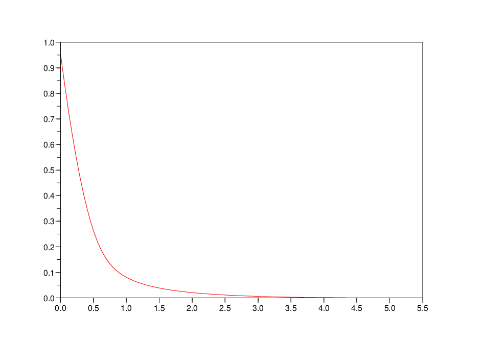
(8) p⁡(t)=∫t+∞(τ−t)​Υ​(τ)​𝑑τ,p(t)=\int_{t}^{+\infty}(\tau-t)\Upsilon(\tau)d\tau\,,

where the function Υ\Upsilon is expressed as follows:

(9) Υ⁡(t)=24π2​{1if ​t∈(0,12],12​t+2​(1−12​t)2​ln⁡(1−12​t)−12​(1−1t)2​ln⁡|1−1t|if ​t∈(12,+∞).\Upsilon(t)=\frac{24}{\pi^{2}}\left\{\begin{array}[]{ll}1&\mbox{if }\ t\in(0,\tfrac{1}{2}],\\ \\ \frac{1}{2t}+2(1-\frac{1}{2t})^{2}\ln(1-\frac{1}{2t})-\frac{1}{2}(1-\frac{1}{t})^{2}\ln|1-\frac{1}{t}|&\mbox{if }\ t\in(\tfrac{1}{2},+\infty)\,.\end{array}\right.

This is precisely at this point that the case of space dimension 22 differs from the higher dimensional case. Indeed, in space dimension higher than 22, the existence of the limit (5) has been proved in [21], while the uniform estimate analogous to (6) is to be found in [17]. However, no explicit formula analogous to (8) is known in that case, at least at the time of this writing. We have chosen to treat in the present paper only the case of the square lattice in space dimension 22 as it is the only case where the limit (5-8) is known completely.

Refer to caption

​​​!​​​​​​​Refer to caption

Figure 1. The graphs of Υ\Upsilon (left) and of pp (right)

Throughout this paper, we assume that the initial data of (Ξε\Xi_{\varepsilon}) satisfies the assumption

(10) fi​n≥0onℝ2×𝕊1and∬ℝ2×𝕊1fi​n(x,v)dxdv+sup(x,v)∈ℝ2×𝕊1fi​n(x,v)<+∞.f^{in}\geq 0\ \mbox{on}\ \mathbbm{R}^{2}\times\mathbb{S}^{1}\ \mbox{and}\iint_{\mathbbm{R}^{2}\times\mathbb{S}^{1}}f^{in}(x,v)dxdv+\sup_{(x,v)\in\mathbbm{R}^{2}\times\mathbb{S}^{1}}f^{in}(x,v)<+\infty.

For each 0<ε≪10<\varepsilon\ll 1, let fεf_{\varepsilon} be the (mild) solution of the initial boundary value problem

(Ξε)​{∂tfε+v⋅∇xfε+σ⁡(fε−K​fε)=0,(x,v)∈Zε×𝕊1,t>0,fε=0,if v⋅nx>0,(x,v)∈∂Zε×𝕊1,fε​(0,x,v)=fi​n​(x,v),(x,v)∈Zε×𝕊1.(\Xi_{\varepsilon})\left\{\begin{array}[]{ll}\partial_{t}f_{\varepsilon}+v\cdot\nabla_{x}f_{\varepsilon}+\sigma(f_{\varepsilon}-Kf_{\varepsilon})=0,&\ (x,v)\in Z_{\varepsilon}\times\mathbb{S}^{1},t>0,\\ \\ f_{\varepsilon}=0,\ \mbox{if\ }v\cdot n_{x}>0,&\ (x,v)\in\partial Z_{\varepsilon}\times\mathbb{S}^{1},\\ \\ f_{\varepsilon}(0,x,v)=f^{in}(x,v),&\ (x,v)\in Z_{\varepsilon}\times\mathbb{S}^{1}.\end{array}\right.

The classical theory of the linear Boltzmann equation guarantees the existence and uniqueness of a mild solution fεf_{\varepsilon} of the problem (Ξε\Xi_{\varepsilon}) satisfying

(11) 0≤fε​(t,x,v)≤sup(x,v)∈ℝ2×𝕊1fi​n​(x,v) a.e. on ​ℝ+×Zε×𝕊1,\displaystyle 0\leq f_{\varepsilon}(t,x,v)\leq\sup_{(x,v)\in\mathbbm{R}^{2}\times\mathbb{S}^{1}}f^{in}(x,v)\quad\hbox{ a.e. on }\mathbbm{R}_{+}\times Z_{\varepsilon}\times\mathbb{S}^{1}\,,
∬Zε×𝕊1fε​(t,x,v)​dx​dv≤∬ℝ2×𝕊1fi​n​(x,v)​dx​dv.\displaystyle\iint_{Z_{\varepsilon}\times\mathbb{S}^{1}}f_{\varepsilon}(t,x,v)dxdv\leq\iint_{\mathbbm{R}^{2}\times\mathbb{S}^{1}}f^{in}(x,v)dxdv\,.

Consider next F:=F⁡(t,s,x,v)F:=F(t,s,x,v) the solution of the Cauchy problem

(Σ)​{∂tF+v⋅∇xF+∂sF=−σ​F+p˙p​(t∧s)​F,t,s>0,(x,v)∈ℝ2×𝕊1,F⁡(t,0,x,v)=σ​∫0+∞K​F​(t,s,x,v)​ds,t>0,(x,v)∈ℝ2×𝕊1,F⁡(0,s,x,v)=σ​e−σ​s​fi​n​(x,v),s>0,(x,v)∈ℝ2×𝕊1,(\Sigma)\left\{\begin{array}[]{ll}\partial_{t}F+v\cdot\nabla_{x}F+\partial_{s}F=-\sigma F+\frac{\dot{p}}{p}(t\wedge s)F,&t,s>0,(x,v)\in\mathbbm{R}^{2}\times\mathbb{S}^{1}\,,\\ \\ F(t,0,x,v)=\sigma\displaystyle\int_{0}^{+\infty}KF(t,s,x,v)ds,&t>0,(x,v)\in\mathbbm{R}^{2}\times\mathbb{S}^{1}\,,\\ \\ F(0,s,x,v)=\sigma e^{-\sigma s}f^{in}(x,v),&s>0,(x,v)\in\mathbbm{R}^{2}\times\mathbb{S}^{1}\,,\end{array}\right.

with the notation t∧s:=min⁡(t,s)t\wedge s:=\min(t,s). Notice that FF is a density defined on the extended phase space:

{(s,x,v)|s≥0,x∈ℝ2,v∈𝕊1}\left\{(s,x,v)|s\geq 0,x\in\mathbbm{R}^{2},v\in\mathbb{S}^{1}\right\}

involving the extra variable ss, whose interpretation is given below.

Henceforth, we shall frequently need to extend functions defined a.e. on ZεZ_{\varepsilon} by 00 inside the holes (that is, in the complement of Zε¯\overline{Z_{\varepsilon}}). We therefore introduce the following piece of notation.

Definition:

For each function φ≡φ⁡(x)\varphi\equiv\varphi(x) defined a.e. on ZεZ_{\varepsilon}, we denote

{φ}​(x)={φ⁡(x)if ​x∈Zε,0if ​x∉Zε¯,\left\{\varphi\right\}(x)=\left\{\begin{array}[]{ll}\varphi(x)&\ \mbox{if }x\in Z_{\varepsilon},\\ 0&\ \mbox{if }x\notin\overline{Z_{\varepsilon}},\end{array}\right.

We use the same notation {fε}\{f_{\varepsilon}\} or {Fε}\{F_{\varepsilon}\} to designate the same extension by 00 inside the holes for functions defined on cartesian products involving ZεZ_{\varepsilon} as one of their factors, such as ℝ+×Zε×𝕊1\mathbbm{R}_{+}\times Z_{\varepsilon}\times\mathbb{S}^{1} in the case of fεf_{\varepsilon}, and ℝ+×ℝ+×Zε×𝕊1\mathbbm{R}_{+}\times\mathbbm{R}_{+}\times Z_{\varepsilon}\times\mathbb{S}^{1} in the case of FεF_{\varepsilon}.

Our first main main result is

Theorem 1.

Under the assumptions above,

{fε}⇀∫0+∞F​𝑑s\{f_{\varepsilon}\}\rightharpoonup\int_{0}^{+\infty}Fds

in L∞​(ℝ+×ℝ2×𝕊1)L^{\infty}(\mathbbm{R}_{+}\times\mathbbm{R}^{2}\times\mathbb{S}^{1}) weak-∗* as ε→0+\varepsilon\rightarrow 0^{+}, where FF is the unique (mild) solution of ( Σ\Sigma).

Notice that the limit of the (extended) distribution function of the particle system is indeed defined in terms of the solution FF of the homogenized integro-differential equation (Σ\Sigma). However, it does not seem that the limit of {fε}\{f_{\varepsilon}\} itself satisfies any natural equation.

Next we discuss the asymptotic decay as t→+∞t\to+\infty of the total mass of the particle system in the homogenization limit ε≪1\varepsilon\ll 1. Obviously, the particle system loses mass due to particles falling into the holes.

In order to do so, we introduce the quantity:

m⁡(t,s):=12​π​∬ℝ2×𝕊1F⁡(t,s,x,v)​𝑑x​𝑑v.m(t,s):=\tfrac{1}{2\pi}\iint_{\mathbbm{R}^{2}\times\mathbb{S}^{1}}F(t,s,x,v)dxdv\,.

A key observation in our work is that mm is the solution of a renewal type PDE, as explained in the next proposition.

Proposition 1.

Denote

B⁡(t,s)=σ−p˙p​(t∧s),B(t,s)=\sigma-\frac{\dot{p}}{p}(t\wedge s)\,,

and assume that fi​nf^{in} satisfies the condition (10).

Then the renewal PDE

{∂tμ⁡(t,s)+∂sμ⁡(t,s)+B⁡(t,s)​μ​(t,s)=0,t,s>0,μ⁡(t,0)=σ​∫0+∞μ⁡(t,s)​ds,t>0,μ⁡(0,s)=σ​e−σ​s,s>0,\left\{\begin{array}[]{ll}\partial_{t}\mu(t,s)+\partial_{s}\mu(t,s)+B(t,s)\mu(t,s)=0,&\ t,s>0\,,\\ \\ \mu(t,0)=\sigma\displaystyle\int_{0}^{+\infty}\mu(t,s)ds,&\ t>0\,,\\ \\ \mu(0,s)=\sigma e^{-\sigma s},&\ s>0\,,\end{array}\right.

has a unique mild solution μ∈L∞​([0,T],L1​(ℝ+))\mu\in L^{\infty}([0,T];L^{1}(\mathbbm{R}_{+})) for all T>0T>0.

Moreover, one has

m⁡(t,s)=μ⁡(t,s)2​π​∬ℝ2×𝕊1fi​n​(x,v)​𝑑x​𝑑vm(t,s)=\frac{\mu(t,s)}{2\pi}\iint_{\mathbbm{R}^{2}\times\mathbb{S}^{1}}f^{in}(x,v)dxdv

a.e. in (t,s)∈ℝ+×ℝ+(t,s)\in\mathbbm{R}_{+}\times\mathbbm{R}_{+}.

Renewal equations are frequently met in many different contexts. For instance they are used as a mathematical model in biology to study the dynamics of structured populations. The interested reader can consult [20] or [24] for more information on this subject.

Consider next the quantity:

(12) M⁡(t):=12​π​∫0+∞∬ℝ2×𝕊1F⁡(t,s,x,v)​𝑑x​𝑑v​𝑑s=∫0+∞m⁡(t,s)​𝑑s.M(t):=\tfrac{1}{2\pi}\int_{0}^{+\infty}\iint_{\mathbbm{R}^{2}\times\mathbb{S}^{1}}F(t,s,x,v)dxdvds=\int_{0}^{+\infty}m(t,s)ds\,.

As explained in the theorem below, M⁡(t)M(t) is the total mass at time tt of the particle system in the limit as ε→0+\varepsilon\to 0^{+}; besides, the asymptotic behavior of MM as t→+∞t\to+\infty is a consequence of the renewal PDE satisfied by the function (t,s)↦m⁡(t,s)(t,s)\mapsto m(t,s).

Theorem 2.

Under the same assumptions as in theorem 1,

  1. (1)

    the total mass

    12​π​∬Zε×𝕊1fε​(t,x,v)​𝑑x​𝑑v→M⁡(t)\tfrac{1}{2\pi}\iint_{Z_{\varepsilon}\times\mathbb{S}^{1}}f_{\varepsilon}(t,x,v)dxdv\rightarrow M(t)

    in Ll​o​c1​(ℝ+)L^{1}_{loc}(\mathbbm{R}_{+}) as ε→0+\varepsilon\to 0^{+}, and a.e. in t≥0t\geq 0 after extracting a subsequence of ε→0+\varepsilon\to 0^{+};

  2. (2)

    the limiting total mass is given by the representation formula

    M⁡(t)=12​π​σ​∬ℝ2×𝕊1fi​n​(x,v)​𝑑x​𝑑v​∑n≥1κ∗n​(t),t>0M(t)=\tfrac{1}{2\pi\sigma}\iint_{\mathbbm{R}^{2}\times\mathbb{S}^{1}}f^{in}(x,v)dxdv\sum_{n\geq 1}\kappa^{*n}(t),\ t>0

    with

    κ⁡(t):=σ​e−σ​t​p​(t)​𝟙t≥0,κ∗n:=κ∗⋯∗κ⏟n factors\kappa(t):=\sigma e^{-\sigma t}p(t)\mathbbm{1}_{t\geq 0}\,,\quad\kappa^{*n}:=\underbrace{\kappa*\cdots*\kappa}_{\hbox{$n$ factors}}

    and ∗* denoting as usual the convolution product on the real line;

  3. (3)

    for each σ>0\sigma>0, there exists ξσ∈(−σ,0)\xi_{\sigma}\in(-\sigma,0) such that

    M⁡(t)∼Cσ​eξσ​t​as​t→+∞M(t)\sim C_{\sigma}e^{\xi_{\sigma}t}\ \mbox{as}\ t\rightarrow+\infty

    with

    Cσ:=12​π​σ​∬ℝ2×𝕊1fi​n​(x,v)​𝑑x​𝑑v∫0∞t​p​(t)​e−(σ+ξσ)​t​𝑑t;C_{\sigma}:=\tfrac{1}{2\pi\sigma}\frac{\displaystyle\iint_{\mathbbm{R}^{2}\times\mathbb{S}^{1}}f^{in}(x,v)dxdv}{\displaystyle\int_{0}^{\infty}tp(t)e^{-(\sigma+\xi_{\sigma})t}dt}\,;
  4. (4)

    finally, the exponential mass loss rate ξσ\xi_{\sigma} satisfies

    ξσ∼−σ​as​σ→0+,and​ξσ→−2​as​σ→+∞.\xi_{\sigma}\sim-\sigma\ \mbox{as}\ \sigma\rightarrow 0^{+},\ \mbox{and}\ \xi_{\sigma}\rightarrow-2\ \mbox{as}\ \sigma\rightarrow+\infty\,.

Statement (1) above means that MM is the limiting mass of the particle system at time tt as ε→0+\varepsilon\to 0^{+}. Statement (3) gives a precise asymptotic equivalent of M⁡(t)M(t) as t→+∞t\to+\infty.

As recalled in the previous section, if σ=0\sigma=0 in the linear Boltzmann equation (Ξε\Xi_{\varepsilon}), the total mass of the particle system in the vanishing ε\varepsilon limit is asymptotically equivalent to

12​π​∬ℝ2×𝕊1fi​n​(x,v)​𝑑x​𝑑vπ2​t\frac{\tfrac{1}{2\pi}\displaystyle\iint_{\mathbbm{R}^{2}\times\mathbb{S}^{1}}f^{in}(x,v)dxdv}{\pi^{2}t}

as t→+∞t\to+\infty. The reason for this slow, algebraic decay is the existence of channels — infinite open strips included in the spatial domain ZεZ_{\varepsilon}, i.e. avoiding all the holes. Particles located in one such channel and moving in a direction close to the channel’s direction will not fall into a hole before exiting the channel, and this can take an arbitrarily long time as the particles’ direction approaches that of the channel. This construction based on channels leads to a sufficiently large fraction of the single-particle phase space and accounts for the algebraic lower bound in (7). The asymptotic equivalent mentioned above in the collisionless case σ=0\sigma=0 is a consequence of a more refined analysis based on continued fractions given in [7].

When σ>0\sigma>0, particles whose distribution function solves the linear Boltzmann equation in (Ξε\Xi_{\varepsilon}) travel on trajectories whose direction is discontinuous in time — more specifically, time discontinuities are distributed under an exponential law of parameter σ\sigma. Obviously, this circumstance destroys the channel structure that is responsible of the algebraic decay of the total mass of the particle system in the collisionless case, so that one expects that the total mass decay is faster than algebraic as t→+∞t\to+\infty. That this decay is indeed exponential whenever σ>0\sigma>0 is by no means obvious: see the argument in [2], leading to an upper bound for the total mass. Statement (3) above leads to an asymptotic equivalent of the total mass, thereby refining the conclusions of [2].

In section 4, we give the proof of theorem 1; the evolution of the total mass in the vanishing ε\varepsilon limit (governing equation and asymptotic behavior as t→+∞t\to+\infty) is discussed in section 5.

4. The homogenized kinetic equation

Our argument for the proof of Theorem 1 is split into several steps.

4.1. A new formulation of the transport equation

Perhaps the most surprising feature in Theorem 1 is the introduction of the extended phase space involving the additional variable ss.

As a matter of fact, this additional variable ss can be used already at the level of the original linear Boltzmann equation — i.e. in the formulation of the problem (Ξε)(\Xi_{\varepsilon}).

Let us indeed return to the initial boundary value problem (Ξε)(\Xi_{\varepsilon}) for the linear Boltzmann equation.

As recalled above, the last two authors have obtained the homogenized equation corresponding to (Ξε)(\Xi_{\varepsilon}) in the noncollisional case (σ=0)(\sigma=0) by explicitly computing the solution of the linear Boltzmann equation for each 0<ε≪10<\varepsilon\ll 1. In the collisionnal case (σ>0)(\sigma>0), as recalled above, there is no such explicit formula giving the solution of the linear Boltzmann equation — except the semi-explicit formula involving the transport process defined in [23].

However, not all the information in that semi-explicit formula is needed for the proof of Theorem 1. The additional variable ss is precisely the exact amount of information contained in that semi-explicit formula needed in the description of the homogenized process in the limit as ε→0+\varepsilon\to 0^{+}.

Consider therefore the initial boundary value problem

(Σε)​{∂tFε+v⋅∇xFε+∂sFε+σ​Fε=0,t,s>0,(x,v)∈Zε×𝕊1,Fε(t,s,x,v)=0,if v⋅nx>0,t,s>0,(x,v)∈(∂Zε×𝕊1),Fε​(t,0,x,v)=σ​∫0∞K​Fε​(t,s,x,v)​ds,t>0,(x,v)∈Zε×𝕊1,Fε​(0,s,x,v)=σ​e−σ​s​fi​n​(x,v),s>0,(x,v)∈Zε×𝕊1,(\Sigma_{\varepsilon})\left\{\begin{array}[]{ll}\partial_{t}F_{\varepsilon}+v\cdot\nabla_{x}F_{\varepsilon}+\partial_{s}F_{\varepsilon}+\sigma F_{\varepsilon}=0,&t,s>0,(x,v)\in Z_{\varepsilon}\times\mathbb{S}^{1},\\ \\ F_{\varepsilon}(t,s,x,v)=0,\ \mbox{if\ }v\cdot n_{x}>0,&t,s>0,(x,v)\in(\partial Z_{\varepsilon}\times\mathbb{S}^{1}),\\ \\ F_{\varepsilon}(t,0,x,v)=\sigma\displaystyle\int_{0}^{\infty}KF_{\varepsilon}(t,s,x,v)ds,&t>0,(x,v)\in Z_{\varepsilon}\times\mathbb{S}^{1},\\ \\ F_{\varepsilon}(0,s,x,v)=\sigma e^{-\sigma s}f^{in}(x,v),&s>0,(x,v)\in Z_{\varepsilon}\times\mathbb{S}^{1},\end{array}\right.

with unknown Fε:=Fε​(t,s,x,v)F_{\varepsilon}:=F_{\varepsilon}(t,s,x,v).

The relation between these two initial boundary value problems, (Ξε)(\Xi_{\varepsilon}) and (Σε)(\Sigma_{\varepsilon}), is explained by the following proposition.

Proposition 2.

Assume that fi​nf^{in} satisfies the assumption (10). Then

a) for each ε>0\varepsilon>0, the problem (Σε)(\Sigma_{\varepsilon}) has a unique mild solution such that

(t,x,v)↦∫0+∞|Fε​(t,s,x,v)|​𝑑s​ belongs to ​L∞​([0,T]×Zε×𝕊1)(t,x,v)\mapsto\int_{0}^{+\infty}|F_{\varepsilon}(t,s,x,v)|ds\hbox{ belongs to }L^{\infty}([0,T]\times Z_{\varepsilon}\times\mathbb{S}^{1})

for each T>0T>0;

b) moreover

0≤Fε​(t,s,x,v)≤‖fi​n‖L∞​(ℝ2×𝕊1)​σ​e−σ​s0\leq F_{\varepsilon}(t,s,x,v)\leq\|f^{in}\|_{L^{\infty}(\mathbbm{R}^{2}\times\mathbb{S}^{1})}\sigma e^{-\sigma s}

a.e. in t,s≥0t,s\geq 0, x∈Zεx\in Z_{\varepsilon} and v∈𝕊1v\in\mathbb{S}^{1}, and

∫0+∞Fε​(t,s,x,v)​𝑑s=fε​(t,x,v),\int_{0}^{+\infty}F_{\varepsilon}(t,s,x,v)ds=f_{\varepsilon}(t,x,v),

for a.e. t≥0,x∈Zε,v∈𝕊1t\geq 0,x\in Z_{\varepsilon},v\in\mathbb{S}^{1}, where fεf_{\varepsilon} is the solution of (Ξε)(\Xi_{\varepsilon}).

Proof.

Applying the method of characteristics, we see that, should a mild solution FεF_{\varepsilon} of the problem (Σε)(\Sigma_{\varepsilon}) exist, it must satisfy

(13) Fε​(t,s,x,v)=F1,ε​(t,s,x,v)+F2,ε​(t,s,x,v),F_{\varepsilon}(t,s,x,v)=F_{1,\varepsilon}(t,s,x,v)+F_{2,\varepsilon}(t,s,x,v),

with

(14) F1,ε​(t,s,x,v)\displaystyle F_{1,\varepsilon}(t,s,x,v) =𝟙s<ε​τε​(xε,v)​𝟙s<t​e−σ​s​Fε​(t−s,0,x−v​s,v)\displaystyle=\mathbbm{1}_{s<\varepsilon\tau_{\varepsilon}(\frac{x}{\varepsilon},v)}\mathbbm{1}_{s<t}e^{-\sigma s}F_{\varepsilon}(t-s,0,x-vs,v)
=𝟙s<ε​τε​(xε,v)​𝟙s<t​σ​e−σ​s​∫0+∞K​Fε​(t−s,τ,x−s​v,v)​𝑑τ\displaystyle=\mathbbm{1}_{s<\varepsilon\tau_{\varepsilon}(\frac{x}{\varepsilon},v)}\mathbbm{1}_{s<t}\sigma e^{-\sigma s}\int_{0}^{+\infty}KF_{\varepsilon}(t-s,\tau,x-sv,v)d\tau

and

(15) F2,ε​(t,s,x,v)\displaystyle F_{2,\varepsilon}(t,s,x,v) =𝟙t<ε​τε​(xε,v)​𝟙t<s​e−σ​t​Fε​(0,s−t,x−v​t,v)\displaystyle=\mathbbm{1}_{t<\varepsilon\tau_{\varepsilon}(\frac{x}{\varepsilon},v)}\mathbbm{1}_{t<s}e^{-\sigma t}F_{\varepsilon}(0,s-t,x-vt,v)
=𝟙t<ε​τε​(xε,v)​𝟙t<s​σ​e−σ​s​fi​n​(x−t​v,v)\displaystyle=\mathbbm{1}_{t<\varepsilon\tau_{\varepsilon}(\frac{x}{\varepsilon},v)}\mathbbm{1}_{t<s}\sigma e^{-\sigma s}f^{in}(x-tv,v)

a.e. in (t,s,x,v)∈ℝ+×ℝ+×ℝ2×𝕊1(t,s,x,v)\in\mathbbm{R}_{+}\times\mathbbm{R}_{+}\times\mathbbm{R}^{2}\times\mathbb{S}^{1}.

First, define 𝒳T\mathcal{X}_{T} to be, for each T>0T>0, the set of measurable functions GG defined on ℝ+×ℝ+×Zε×𝕊1\mathbbm{R}_{+}\times\mathbbm{R}_{+}\times Z_{\varepsilon}\times\mathbb{S}^{1} such that

(t,x,v)↦∫0+∞|G⁡(t,s,x,v)|​𝑑s​ belongs to ​L∞​([0,T]×Zε×𝕊1),(t,x,v)\mapsto\int_{0}^{+\infty}|G(t,s,x,v)|ds\hbox{ belongs to }L^{\infty}([0,T]\times Z_{\varepsilon}\times\mathbb{S}^{1})\,,

which is a Banach space for the norm

‖G‖𝒳T=‖∫0+∞|G⁡(⋅,s,⋅,⋅)|​𝑑s‖L∞​([0,T]×Zε×𝕊1).\|G\|_{\mathcal{X}_{T}}=\left\|\int_{0}^{+\infty}|G(\cdot,s,\cdot,\cdot)|ds\right\|_{L^{\infty}([0,T]\times Z_{\varepsilon}\times\mathbb{S}^{1})}\,.

Next, for each G∈𝒳TG\in\mathcal{X}_{T}, we define

𝒯​G​(t,s,x,v):=𝟙s<ε​τε​(xε,v)​𝟙s<t​σ​e−σ​s​∫0+∞K​G​(t−s,τ,x−s​v,v)​𝑑τ.\mathcal{T}G(t,s,x,v):=\mathbbm{1}_{s<\varepsilon\tau_{\varepsilon}(\frac{x}{\varepsilon},v)}\mathbbm{1}_{s<t}\sigma e^{-\sigma s}\int_{0}^{+\infty}KG(t-s,\tau,x-sv,v)d\tau\,.

Obviously

‖∫0+∞|𝒯nG(t,s,⋅,⋅)|ds‖L∞​(Zε×𝕊1)\displaystyle\left\|\int_{0}^{+\infty}|\mathcal{T}^{n}G(t,s,\cdot,\cdot)|ds\right\|_{L^{\infty}(Z_{\varepsilon}\times\mathbb{S}^{1})}
≤σ∫0t‖∫0+∞|𝒯n−1G(t1,τ,⋅,⋅)|dτ‖L∞​(Zε×𝕊1)dt1\displaystyle\leq\sigma\int_{0}^{t}\left\|\int_{0}^{+\infty}|\mathcal{T}^{n-1}G(t_{1},\tau,\cdot,\cdot)|d\tau\right\|_{L^{\infty}(Z_{\varepsilon}\times\mathbb{S}^{1})}dt_{1}
≤σn∫0t…∫0tn−1‖∫0+∞|G(tn,s,⋅,⋅)|ds‖L∞​(Zε×𝕊1)dtn…dt1,\displaystyle\leq\sigma^{n}\int_{0}^{t}\ldots\int_{0}^{t_{n-1}}\left\|\int_{0}^{+\infty}|G(t_{n},s,\cdot,\cdot)|ds\right\|_{L^{\infty}(Z_{\varepsilon}\times\mathbb{S}^{1})}dt_{n}\ldots dt_{1}\,,

so that

‖𝒯n​G‖𝒳T≤(σ​T)nn!​‖𝒯n​G‖𝒳T.\|\mathcal{T}^{n}G\|_{\mathcal{X}_{T}}\leq\frac{(\sigma T)^{n}}{n!}\|\mathcal{T}^{n}G\|_{\mathcal{X}_{T}}\,.

Now F1,ε=𝒯​FεF_{1,\varepsilon}=\mathcal{T}F_{\varepsilon}, so that (13) can be recast as

Fε=F2,ε+𝒯​Fε.F_{\varepsilon}=F_{2,\varepsilon}+\mathcal{T}F_{\varepsilon}\,.

This integral equation has a solution Fε∈𝒳TF_{\varepsilon}\in\mathcal{X}_{T} for each T>0T>0, given by the series

Fε=∑n≥0𝒯n​F2,εF_{\varepsilon}=\sum_{n\geq 0}\mathcal{T}^{n}F_{2,\varepsilon}

which is normally convergent in the Banach space 𝒳T\mathcal{X}_{T} since

∑n≥0‖𝒯n​F2,ε‖𝒳T≤∑n≥0(σ​T)nn!​‖F2,ε‖𝒳T<+∞.\sum_{n\geq 0}\|\mathcal{T}^{n}F_{2,\varepsilon}\|_{\mathcal{X}_{T}}\leq\sum_{n\geq 0}\frac{(\sigma T)^{n}}{n!}\|F_{2,\varepsilon}\|_{\mathcal{X}_{T}}<+\infty\,.

Assuming that the integral equation above has another solution Fε′∈𝒳TF^{\prime}_{\varepsilon}\in\mathcal{X}_{T} would imply that

Fε−Fε′=𝒯⁡(Fε−Fε′)=…=𝒯n​(Fε−Fε′),F_{\varepsilon}-F^{\prime}_{\varepsilon}=\mathcal{T}(F_{\varepsilon}-F^{\prime}_{\varepsilon})=\ldots=\mathcal{T}^{n}(F_{\varepsilon}-F^{\prime}_{\varepsilon})\,,

so that

‖Fε−Fε′‖𝒳T=‖𝒯n​(Fε−Fε′)‖𝒳T≤(σ​T)nn!​‖Fε−Fε′‖𝒳T→0\|F_{\varepsilon}-F^{\prime}_{\varepsilon}\|_{\mathcal{X}_{T}}=\|\mathcal{T}^{n}(F_{\varepsilon}-F^{\prime}_{\varepsilon})\|_{\mathcal{X}_{T}}\leq\frac{(\sigma T)^{n}}{n!}\|F_{\varepsilon}-F^{\prime}_{\varepsilon}\|_{\mathcal{X}_{T}}\to 0

as n→+∞n\to+\infty: hence Fε′=FεF^{\prime}_{\varepsilon}=F_{\varepsilon}. Thus we have proved statement a).

As for statement b), observe that 𝒯​G≥0\mathcal{T}G\geq 0 a.e. on ℝ+×ℝ+×Zε×𝕊1\mathbbm{R}_{+}\times\mathbbm{R}_{+}\times Z_{\varepsilon}\times\mathbb{S}^{1} if G≥0G\geq 0 a.e. on ℝ+×ℝ+×Zε×𝕊1\mathbbm{R}_{+}\times\mathbbm{R}_{+}\times Z_{\varepsilon}\times\mathbb{S}^{1}. Hence, if fi​n∈L∞​(ℝ2×𝕊1)f^{in}\in L^{\infty}(\mathbbm{R}^{2}\times\mathbb{S}^{1}) satisfies fi​n≥0f^{in}\geq 0 a.e. on ℝ2×𝕊1\mathbbm{R}^{2}\times\mathbb{S}^{1}, one has F2,ε≥0F_{2,\varepsilon}\geq 0 a.e. on ℝ+×ℝ+×Zε×𝕊1\mathbbm{R}_{+}\times\mathbbm{R}_{+}\times Z_{\varepsilon}\times\mathbb{S}^{1}, so that 𝒯n​F2,ε≥0\mathcal{T}^{n}F_{2,\varepsilon}\geq 0 a.e. on ℝ+×ℝ+×Zε×𝕊1\mathbbm{R}_{+}\times\mathbbm{R}_{+}\times Z_{\varepsilon}\times\mathbb{S}^{1} and the series defining FεF_{\varepsilon} is a.e. nonnegative on ℝ+×ℝ+×Zε×𝕊1\mathbbm{R}_{+}\times\mathbbm{R}_{+}\times Z_{\varepsilon}\times\mathbb{S}^{1}.

Next, integrating both sides of (13) with respect to ss, and setting

gε​(t,x,v):=∫0+∞Fε​(t,s,x,v)​𝑑s,g_{\varepsilon}(t,x,v):=\int_{0}^{+\infty}F_{\varepsilon}(t,s,x,v)ds\,,

we arrive at

gε​(t,x,v)\displaystyle g_{\varepsilon}(t,x,v) =∫0+∞F2,ε​(t,s,x,v)​𝑑s+∫0+∞F1,ε​(t,s,x,v)​𝑑s\displaystyle=\int_{0}^{+\infty}F_{2,\varepsilon}(t,s,x,v)ds+\int_{0}^{+\infty}F_{1,\varepsilon}(t,s,x,v)ds
=𝟙t<ε​τε​(xε,v)​fi​n​(x−t​v,v)​∫0+∞𝟙t<s​σ​e−σ​s​𝑑s\displaystyle=\mathbbm{1}_{t<\varepsilon\tau_{\varepsilon}(\frac{x}{\varepsilon},v)}f^{in}(x-tv,v)\int_{0}^{+\infty}\mathbbm{1}_{t<s}\sigma e^{-\sigma s}ds
+∫0+∞𝟙s<ε​τε​(xε,v)𝟙s<tσe−σ​s(∫0+∞KFε(t−s,τ,x−sv,v)dτ)ds\displaystyle+\int_{0}^{+\infty}\mathbbm{1}_{s<\varepsilon\tau_{\varepsilon}(\frac{x}{\varepsilon},v)}\mathbbm{1}_{s<t}\sigma e^{-\sigma s}\left(\int_{0}^{+\infty}KF_{\varepsilon}(t-s,\tau,x-sv,v)d\tau\right)ds
=𝟙t<ε​τε​(xε,v)​fi​n​(x−t​v,v)​e−σ​t\displaystyle=\mathbbm{1}_{t<\varepsilon\tau_{\varepsilon}(\frac{x}{\varepsilon},v)}f^{in}(x-tv,v)e^{-\sigma t}
+∫0te−σ​s𝟙s<ε​τε​(xε,v)σKgε(t−s,x−sv,v)ds\displaystyle+\int_{0}^{t}e^{-\sigma s}\mathbbm{1}_{s<\varepsilon\tau_{\varepsilon}(\frac{x}{\varepsilon},v)}\sigma Kg_{\varepsilon}(t-s,x-sv,v)ds

in which we recognize the Duhamel formula giving the unique mild solution fεf_{\varepsilon} of (Ξε)(\Xi_{\varepsilon}). Hence

fε​(t,x,v)=∫0+∞Fε​(t,s,x,v)​𝑑s​ a.e. in ​(t,x,v)∈ℝ+×Zε×𝕊1.f_{\varepsilon}(t,x,v)=\int_{0}^{+\infty}F_{\varepsilon}(t,s,x,v)ds\hbox{ a.e. in }(t,x,v)\in\mathbbm{R}_{+}\times Z_{\varepsilon}\times\mathbb{S}^{1}\,.

Finally, since (Ξε)(\Xi_{\varepsilon}) satisfies the maximum principle, one has

fε​(t,x,v)≤‖fi​n‖L∞​(ℝ2×𝕊1)​ a.e. in ​(t,x,v)∈ℝ+×Zε×𝕊1.f_{\varepsilon}(t,x,v)\leq\|f^{in}\|_{L^{\infty}(\mathbbm{R}^{2}\times\mathbb{S}^{1})}\hbox{ a.e. in }(t,x,v)\in\mathbbm{R}_{+}\times Z_{\varepsilon}\times\mathbb{S}^{1}\,.

Going back to (13), we recast it in the form

Fε​(t,s,x,v)\displaystyle F_{\varepsilon}(t,s,x,v) =𝟙s<ε​τε​(xε,v)​𝟙s<t​σ​e−σ​s​K​fε​(t−s,x−s​v,v)\displaystyle=\mathbbm{1}_{s<\varepsilon\tau_{\varepsilon}(\frac{x}{\varepsilon},v)}\mathbbm{1}_{s<t}\sigma e^{-\sigma s}Kf_{\varepsilon}(t-s,x-sv,v)
+𝟙t<ε​τε​(xε,v)​𝟙t<s​σ​e−σ​s​fi​n​(x−t​v,v)\displaystyle+\mathbbm{1}_{t<\varepsilon\tau_{\varepsilon}(\frac{x}{\varepsilon},v)}\mathbbm{1}_{t<s}\sigma e^{-\sigma s}f^{in}(x-tv,v)
≤𝟙s<ε​τε​(xε,v)​𝟙s<t​σ​e−σ​s​‖fi​n‖L∞​(ℝ2×𝕊1)\displaystyle\leq\mathbbm{1}_{s<\varepsilon\tau_{\varepsilon}(\frac{x}{\varepsilon},v)}\mathbbm{1}_{s<t}\sigma e^{-\sigma s}\|f^{in}\|_{L^{\infty}(\mathbbm{R}^{2}\times\mathbb{S}^{1})}
+𝟙t<ε​τε​(xε,v)​𝟙t<s​σ​e−σ​s​‖fi​n‖L∞​(ℝ2×𝕊1)\displaystyle+\mathbbm{1}_{t<\varepsilon\tau_{\varepsilon}(\frac{x}{\varepsilon},v)}\mathbbm{1}_{t<s}\sigma e^{-\sigma s}\|f^{in}\|_{L^{\infty}(\mathbbm{R}^{2}\times\mathbb{S}^{1})}
≤σ​e−σ​s​‖fi​n‖L∞​(ℝ2×𝕊1)\displaystyle\leq\sigma e^{-\sigma s}\|f^{in}\|_{L^{\infty}(\mathbbm{R}^{2}\times\mathbb{S}^{1})}

a.e. in (t,s,x,v)∈ℝ+×ℝ+×Zε×𝕊1(t,s,x,v)\in\mathbbm{R}_{+}\times\mathbbm{R}_{+}\times Z_{\varepsilon}\times\mathbb{S}^{1}, which concludes the proof. ∎

Observe that if

Fε​(0,s,x,v)=σ​e−σ​s​fi​n​(x,v)F_{\varepsilon}(0,s,x,v)=\sigma e^{-\sigma s}f^{in}(x,v)

is replaced with

Fε​(0,s,x,v)=Π⁡(s)​fi​n​(x,v)F_{\varepsilon}(0,s,x,v)=\Pi(s)f^{in}(x,v)

where Π\Pi is any probability density on ℝ+\mathbbm{R}_{+} vanishing at ∞\infty, the conclusion of the lemma above remains valid. In other words, the dependence of the solution FεF_{\varepsilon} of the problem (Σ\Sigma) upon the choice of the initial probability density Π\Pi disappears after integration in ss, so that the particle distribution function fεf_{\varepsilon} is indeed independent of the choice of Π\Pi.

The extra variable ss in the extended phase space has the following interpretation. Recall that the solution fεf_{\varepsilon} of the linear Boltzmann equation can be expressed in terms of the transport process (see [23]), a stochastic process involving a jump process in the vv variable, perturbed by a drift in the xx variable. The variable ss is the “age” of the current velocity vv in that process, i.e. the time since the last jump in the vv variable.

The choice Π⁡(s)=σ​e−σ​s\Pi(s)=\sigma e^{-\sigma s} corresponds with the situation where the gas molecules have been evolving under the linear Boltzmann equation for t<0t<0 and the holes are suddenly opened at t=0t=0.

Before giving the proof of Theorem 1, we need to establish a few technical lemmas.

4.2. The distribution of free path lengths

A straightforward consequence of the limit in (5) is the following lemma, which accounts eventually for the coefficient p˙​(t∧s)/p​(t∧s)\dot{p}(t\wedge s)/p(t\wedge s) in the limiting equation (Σ\Sigma).

Lemma 1.

Let τε\tau_{\varepsilon} be the free path length defined in (4)(\ref{length}). Then for each t>0t>0

{𝟙t<ε​τε​(xε,v)}⇀p⁡(t)\{\mathbbm{1}_{t<\varepsilon\tau_{\varepsilon}(\frac{x}{\varepsilon},v)}\}\rightharpoonup p(t)

in L∞​(ℝ2×𝕊1)L^{\infty}(\mathbbm{R}^{2}\times\mathbb{S}^{1}) weak-∗* as ε→0+\varepsilon\rightarrow 0^{+}.

(See the definition before Theorem 1 for the notation {𝟙t<ε​τε​(xε,v)}\{\mathbbm{1}_{t<\varepsilon\tau_{\varepsilon}(\frac{x}{\varepsilon},v)}\}.)

Proof.

Since the linear span of functions χ≡χ⁡(x,v)\chi\equiv\chi(x,v) of the form

ϕ⁡(x,v)=χ⁡(x)​𝟙I​(v),ϕ∈C0∞​(ℝ2)​ and I an arc of 𝕊1\phi(x,v)=\chi(x)\mathbbm{1}_{I}(v)\,,\quad\phi\in C^{\infty}_{0}(\mathbbm{R}^{2})\hbox{ and $I$ an arc of $\mathbb{S}^{1}$}

is dense in L1​(ℝ2×𝕊1)L^{1}(\mathbbm{R}^{2}\times\mathbb{S}^{1}), and the family 𝟙ε​τε​(xε,v)>t\mathbbm{1}_{\varepsilon\tau_{\varepsilon}(\frac{x}{\varepsilon},v)>t} is bounded in L∞​(ℝ2×𝕊1)L^{\infty}(\mathbbm{R}^{2}\times\mathbb{S}^{1}), it is enough to prove that

∬Zε×𝕊1ϕ⁡(x,v)​𝟙ε​τε​(xε,v)>t​𝑑x​𝑑v→p⁡(t)​∬ℝ2×𝕊1ϕ⁡(x,v)​𝑑x​𝑑v​as ​ε→0.\iint_{Z_{\varepsilon}\times\mathbb{S}^{1}}\phi(x,v)\mathbbm{1}_{\varepsilon\tau_{\varepsilon}(\frac{x}{\varepsilon},v)>t}dxdv\rightarrow p(t)\iint_{\mathbbm{R}^{2}\times\mathbb{S}^{1}}\phi(x,v)dxdv\ \mbox{as\ }\varepsilon\rightarrow 0\,.

Write

∬Zε×𝕊1ϕ⁡(x,v)​𝟙ε​τε​(xε,v)>t​𝑑x​𝑑v\displaystyle\iint_{Z_{\varepsilon}\times\mathbb{S}^{1}}\phi(x,v)\mathbbm{1}_{\varepsilon\tau_{\varepsilon}(\frac{x}{\varepsilon},v)>t}dxdv =\displaystyle= ∫Zεχ⁡(x)​(∫I𝟙ε​τε​(xε,v)>t​𝑑v)​𝑑x\displaystyle\int_{Z_{\varepsilon}}\chi(x)\left(\int_{I}\mathbbm{1}_{\varepsilon\tau_{\varepsilon}(\frac{x}{\varepsilon},v)>t}dv\right)dx
=\displaystyle= ∫Zεχ⁡(x)​Tε​(xε)​𝑑x\displaystyle\int_{Z_{\varepsilon}}\chi(x)T_{\varepsilon}\left(\frac{x}{\varepsilon}\right)dx

with

Tε​(y):=∫I𝟙ε​τε​(y,v)>t​𝑑v.T_{\varepsilon}(y):=\int_{I}\mathbbm{1}_{\varepsilon\tau_{\varepsilon}(y,v)>t}dv\,.

Obviously TεT_{\varepsilon} is 11-periodic in y1y_{1} and y2y_{2} and satisfies 0≤Tε≤|I|0\leq T_{\varepsilon}\leq|I|. Hence

𝟙d⁡(y,ℤ2)>ε​Tε​(y)=∑k∈ℤ2T^ε​(k)​e2​i​π​k⋅y\mathbbm{1}_{d(y,\mathbbm{Z}^{2})>\varepsilon}T_{\varepsilon}(y)=\sum_{k\in\mathbbm{Z}^{2}}\hat{T}_{\varepsilon}(k)e^{2i\pi k\cdot y}

in L2​(ℝ2/ℤ2)L^{2}(\mathbbm{R}^{2}/\mathbbm{Z}^{2}) with

T^ε(k):=∫max⁡(|z1|,|z2|)<1/2|z|>εTε(z)−2iπk⋅zdz\hat{T}_{\varepsilon}(k):=\int_{\max(|z_{1}|,|z_{2}|)<1/2\atop|z|>\varepsilon}T_{\varepsilon}(z)^{-2i\pi k\cdot z}dz

for each k∈ℤ2k\in\mathbbm{Z}^{2}.

Then, by Parseval’s identity,

∫Zεχ⁡(x)​Tε​(xε)​𝑑x\displaystyle\int_{Z_{\varepsilon}}\chi(x)T_{\varepsilon}\left(\frac{x}{\varepsilon}\right)dx =∫ℝ2χ⁡(x)​(∑k∈ℤ2T^ε​(k)​e2​i​π​k⋅xε)​𝑑x\displaystyle=\int_{\mathbbm{R}^{2}}\chi(x)\left(\sum_{k\in\mathbbm{Z}^{2}}\hat{T}_{\varepsilon}(k)e^{2i\pi\frac{k\cdot x}{\varepsilon}}\right)dx
=χ^(0)T^ε(0)+∑k∈ℤ2∖(0,0)T^ε(k)χ^(−2πk/ε),\displaystyle=\hat{\chi}(0)\hat{T}_{\varepsilon}(0)+\sum_{k\in\mathbbm{Z}^{2}\setminus(0,0)}\hat{T}_{\varepsilon}(k)\hat{\chi}(-2\pi k/\varepsilon)\,,

with

χ^(ξ):=∫ℝ2χ(x)e−iξ⋅xdx.\hat{\chi}(\xi):=\int_{\mathbbm{R}^{2}}\chi(x)e^{-i\xi\cdot x}dx\,.

Applying again Parseval’s identity,

∑k∈ℤ2|T^ε​(k)|2=∫max⁡(|y1|,|y2|)<1/2|y|>ε|Tε​(y)|2​𝑑y≤|I|\sum_{k\in\mathbbm{Z}^{2}}|\hat{T}_{\varepsilon}(k)|^{2}=\int_{\max(|y_{1}|,|y_{2}|)<1/2\atop|y|>\varepsilon}|T_{\varepsilon}(y)|^{2}dy\leq|I|

while

|χ^​(ξ)|≤1|ξ|2​‖∇2χ‖L∞,|\hat{\chi}(\xi)|\leq\frac{1}{|\xi|^{2}}\|\nabla^{2}\chi\|_{L^{\infty}}\,,

so that

|χ^(−2πk/ε)|≤ε24​π2​|ξ|2∥∇2χ∥L∞.|\hat{\chi}(-2\pi k/\varepsilon)|\leq\frac{\varepsilon^{2}}{4\pi^{2}|\xi|^{2}}\|\nabla^{2}\chi\|_{L^{\infty}}\,.

Hence, by the Cauchy-Schwarz inequality,

|∑k∈ℤ2∖(0,0)T^ε(k)χ^(−2πk/ε)|2≤∑k∈ℤ2∖(0,0)|T^ε(k)|2∑k∈ℤ2∖(0,0)ε4​‖∇2χ‖L∞216​π4​|k|4=O(ε4)\left|\sum_{k\in\mathbbm{Z}^{2}\setminus(0,0)}\hat{T}_{\varepsilon}(k)\hat{\chi}(-2\pi k/\varepsilon)\right|^{2}\leq\sum_{k\in\mathbbm{Z}^{2}\setminus(0,0)}|\hat{T}_{\varepsilon}(k)|^{2}\sum_{k\in\mathbbm{Z}^{2}\setminus(0,0)}\frac{\varepsilon^{4}\|\nabla^{2}\chi\|^{2}_{L^{\infty}}}{16\pi^{4}|k|^{4}}=O(\varepsilon^{4})

and therefore

∫Zεχ⁡(x)​Tε​(xε)​𝑑x=χ^​(0)​T^ε​(0)+O⁡(ε2)\int_{Z_{\varepsilon}}\chi(x)T_{\varepsilon}\left(\frac{x}{\varepsilon}\right)dx=\hat{\chi}(0)\hat{T}_{\varepsilon}(0)+O(\varepsilon^{2})

as ε→0+\varepsilon\to 0^{+}.

By (5)

T^ε​(0)=∫max⁡(|y1|,|y2|)<1/2|y|>εTε​(y)​𝑑y→p⁡(t)​|I|Êas ​ε→0+,\hat{T}_{\varepsilon}(0)=\int_{\max(|y_{1}|,|y_{2}|)<1/2\atop|y|>\varepsilon}T_{\varepsilon}(y)dy\to p(t)|I|\quad\hbox{Êas }\varepsilon\to 0^{+}\,,

so that

χ^​(0)​T^ε​(0)→p⁡(t)|I|∫ℝ2χ⁡(x)​𝑑x=p⁡(t)​∬ℝ2×𝕊1ϕ⁡(x,v)​𝑑x​𝑑v\hat{\chi}(0)\hat{T}_{\varepsilon}(0)\to p(t)|I|\int_{\mathbbm{R}^{2}}\chi(x)dx=p(t)\iint_{\mathbbm{R}^{2}\times\mathbb{S}^{1}}\phi(x,v)dxdv

as ε→0+\varepsilon\to 0^{+}, and hence

∫Zεχ⁡(x)​Tε​(xε)​𝑑x=p⁡(t)​∬ℝ2×𝕊1ϕ⁡(x,v)​𝑑x​𝑑v+o⁡(1)+O⁡(ε2)\int_{Z_{\varepsilon}}\chi(x)T_{\varepsilon}\left(\frac{x}{\varepsilon}\right)dx=p(t)\iint_{\mathbbm{R}^{2}\times\mathbb{S}^{1}}\phi(x,v)dxdv+o(1)+O(\varepsilon^{2})

which entails the announced result. ∎

4.3. Extending fεf_{\varepsilon} by 00 in the holes

We begin with the equation satisfied by the (extension by 00 inside the holes of the) distribution function {fε}\left\{f_{\varepsilon}\right\}.

Lemma 2.

For each ε>0\varepsilon>0, the function {fε}\left\{f_{\varepsilon}\right\} satisfies

(∂t+v⋅∇x){fε}+σ({fε}−K{fε})=(v⋅nx)fε|∂Zε×𝕊1δ∂Zε(\partial_{t}+v\cdot\nabla_{x})\left\{f_{\varepsilon}\right\}+\sigma(\left\{f_{\varepsilon}\right\}-K\left\{f_{\varepsilon}\right\})=(v\cdot n_{x})f_{\varepsilon}\big|_{\partial Z_{\varepsilon}\times\mathbb{S}^{1}}\delta_{\partial Z_{\varepsilon}}

in 𝒟′​(ℝ+∗×ℝ2×𝕊1),\mathcal{D}^{\prime}(\mathbbm{R}_{+}^{*}\times\mathbbm{R}^{2}\times\mathbb{S}^{1}), where δ∂Zε\delta_{\partial Z_{\varepsilon}} is the surface measure concentrated on the boundary of ZεZ_{\varepsilon}, and nxn_{x} is the unit normal vector at x∈∂Zεx\in\partial Z_{\varepsilon} pointing towards the interior of ZεZ_{\varepsilon}.

Proof.

One has

∂t{fε}={∂tfε}\partial_{t}\left\{f_{\varepsilon}\right\}=\left\{\partial_{t}f_{\varepsilon}\right\}

and

∇x{fε}={∇xfε}+fε∣∂Zε×𝕊1​δ∂Zε​nx\nabla_{x}\left\{f_{\varepsilon}\right\}=\left\{\nabla_{x}f_{\varepsilon}\right\}+f_{\varepsilon}\mid_{\partial Z_{\varepsilon}\times\mathbb{S}^{1}}\delta_{\partial Z_{\varepsilon}}n_{x}

in 𝒟′​(ℝ+∗×ℝ2×𝕊1)\mathcal{D}^{\prime}(\mathbbm{R}_{+}^{*}\times\mathbbm{R}^{2}\times\mathbb{S}^{1}). Hence

0\displaystyle 0 =\displaystyle= {∂tfε+v⋅∇xfε+σ⁡(fε−K​fε)}\displaystyle\left\{\partial_{t}f_{\varepsilon}+v\cdot\nabla_{x}f_{\varepsilon}+\sigma(f_{\varepsilon}-Kf_{\varepsilon})\right\}
=\displaystyle= ∂t{fε}+v⋅∇x{fε}+(v⋅nx)​fε|∂Zε×𝕊1​δ∂Zε+σ⁡({fε}−K⁡{fε})\displaystyle\partial_{t}\left\{f_{\varepsilon}\right\}+v\cdot\nabla_{x}\left\{f_{\varepsilon}\right\}+(v\cdot n_{x})f_{\varepsilon}\big|_{\partial Z_{\varepsilon}\times\mathbb{S}^{1}}\delta_{\partial Z_{\varepsilon}}+\sigma(\left\{f_{\varepsilon}\right\}-K\left\{f_{\varepsilon}\right\})

in 𝒟′​(ℝ+∗×ℝ2×𝕊1)\mathcal{D}^{\prime}(\mathbbm{R}_{+}^{*}\times\mathbbm{R}^{2}\times\mathbb{S}^{1}). ∎

A straightforward consequence of the scaling considered here is that the family of Radon measures

(v⋅nx)​fε|∂Zε×𝕊1​δ∂Zε(v\cdot n_{x})f_{\varepsilon}\big|_{\partial Z_{\varepsilon}\times\mathbb{S}^{1}}\delta_{\partial Z_{\varepsilon}}

is controlled uniformly as ε→0+\varepsilon\rightarrow 0^{+}, in the following manner.

Lemma 3.

For each R>0R>0, the family of Radon measures

(v⋅nx)​fε|∂Zε×𝕊1​δ∂Zε|[−R,R]2×𝕊1(v\cdot n_{x})f_{\varepsilon}\big|_{\partial Z_{\varepsilon}\times\mathbb{S}^{1}}\delta_{\partial Z_{\varepsilon}}\big|_{[-R,R]^{2}\times\mathbb{S}^{1}}

is bounded in11 1 For each compact subset KK of ℝN\mathbbm{R}^{N}, we denote by ℳ⁡(K)\mathcal{M}(K) the space of signed Radon measures on KK, i.e. the set of all real-valued continuous linear functionals on C⁡(K)C(K) endowed with the topology of uniform convergence on KK. ℳ⁡([−R,R]2×𝕊1)\mathcal{M}([-R,R]^{2}\times\mathbb{S}^{1}).

Proof.

The total mass of the measure

(v⋅nx)​fε|∂Zε×𝕊1​δ∂Zε|[−R,R]2×𝕊1(v\cdot n_{x})f_{\varepsilon}\big|_{\partial Z_{\varepsilon}\times\mathbb{S}^{1}}\delta_{\partial Z_{\varepsilon}}\big|_{[-R,R]^{2}\times\mathbb{S}^{1}}

is less than or equal to

2​π​‖fε‖L∞​(ℝ+×Zε×𝕊1)​‖δ∂Zε∣[−R,R]2‖ℳ⁡([−R,R]2)2\pi\|f_{\varepsilon}\|_{L^{\infty}(\mathbbm{R}_{+}\times Z_{\varepsilon}\times\mathbb{S}^{1})}\|\delta_{\partial Z_{\varepsilon}}\mid_{[-R,R]^{2}}\|_{\mathcal{M}([-R,R]^{2})}

which is itself less than or equal to

2​π​‖fi​n‖L∞​(ℝ2×𝕊1)​‖δ∂Zε∣[−R,R]2‖ℳ⁡([−R,R]2).2\pi\|f^{in}\|_{L^{\infty}(\mathbbm{R}^{2}\times\mathbb{S}^{1})}\left\|\delta_{\partial Z_{\varepsilon}}\mid_{[-R,R]^{2}}\right\|_{\mathcal{M}([-R,R]^{2})}\,.

Since δ∂Zε∣[−R,R]2\delta_{\partial Z_{\varepsilon}}\mid_{[-R,R]^{2}} is the union of O⁡((2​Rε)2)O\left(\left(\frac{2R}{\varepsilon}\right)^{2}\right) circles of radius ε2\varepsilon^{2},

‖δ∂Zε∣[−R,R]2‖ℳ⁡([−R,R]2)=O⁡((2​Rε)2)​2​π​ε2=O⁡(1)​R2\|\delta_{\partial Z_{\varepsilon}}\mid_{[-R,R]^{2}}\|_{\mathcal{M}([-R,R]^{2})}=O\left(\left(\frac{2R}{\varepsilon}\right)^{2}\right)2\pi\varepsilon^{2}=O(1)R^{2}

as ε→0+\varepsilon\to 0^{+}, whence the announced result. ∎

4.4. The velocity averaging lemmas

As is the case of all homogenization results, the proof of Theorem 1 is based on the strong Ll​o​c1L^{1}_{loc} convergence of certain quantities defined in terms of FεF_{\varepsilon}. In the case of kinetic models, strong Ll​o​c1L^{1}_{loc} compactness is usually obtained by velocity averaging — see for instance [1, 19, 18] for the first results in this direction. Below, we recall a classical result in velocity averaging that is a special case of theorem 1.8 in [5].

Proposition 3.

Let p>1p>1 and assume that fε≡fε​(t,x,v)f_{\varepsilon}\equiv f_{\varepsilon}(t,x,v) is a bounded family in Ll​o​cp​(ℝt+×ℝxd×𝕊vd−1)L^{p}_{loc}(\mathbbm{R}^{+}_{t}\times\mathbbm{R}^{d}_{x}\times\mathbb{S}^{d-1}_{v}) such that

supε∫0T∬B⁡(0,R)×𝕊d−1|∂tfε+v⋅∇xfε|​𝑑x​𝑑v​𝑑t<+∞\sup_{\varepsilon}\int_{0}^{T}\iint_{B(0,R)\times\mathbb{S}^{d-1}}|\partial_{t}f_{\varepsilon}+v\cdot\nabla_{x}f_{\varepsilon}|dxdvdt<+\infty

for each T>0T>0 and R>0R>0. Then, for each ψ∈C⁡(𝕊d−1×𝕊d−1)\psi\in C(\mathbb{S}^{d-1}\times\mathbb{S}^{d-1}), the family ρψ​[fε]\rho_{\psi}[f_{\varepsilon}], defined by

ρψ​[fε]​(t,x,v)=∫𝕊d−1fε​(t,x,v)​ψ​(v,w)​𝑑w\rho_{\psi}[f_{\varepsilon}](t,x,v)=\int_{\mathbb{S}^{d-1}}f_{\varepsilon}(t,x,v)\psi(v,w)dw

is relatively compact in Ll​o​c1​(ℝt+×ℝxd×𝕊vd−1)L^{1}_{loc}(\mathbbm{R}^{+}_{t}\times\mathbbm{R}^{d}_{x}\times\mathbb{S}^{d-1}_{v}).

A straightforward consequence of Proposition 3 is the following compactness result in Ll​o​c1L^{1}_{loc} strong, which is the key argument in the proof of Theorem 1.

Lemma 4.

Let fε≡fε​(t,x,v)f_{\varepsilon}\equiv f_{\varepsilon}(t,x,v) be the family of solutions of the initial boundary value problem (Ξε)(\Xi_{\varepsilon}). Then the families

K⁡{fε}={K​fε}K\left\{f_{\varepsilon}\right\}=\left\{Kf_{\varepsilon}\right\}

and

∫𝕊1{fε}​𝑑v\int_{\mathbb{S}^{1}}\{f_{\varepsilon}\}dv

are relatively compact in Ll​o​c1​(ℝ+×ℝ2×𝕊1)L^{1}_{loc}(\mathbbm{R}_{+}\times\mathbbm{R}^{2}\times\mathbb{S}^{1}) strong.

Proof.

We recall that, by the Maximum Principle for (Ξε)(\Xi_{\varepsilon}),

|fε​(t,x,v)|≤‖fi​n‖L∞​(ℝ2×𝕊1)|f_{\varepsilon}(t,x,v)|\leq\|f^{in}\|_{L^{\infty}(\mathbbm{R}^{2}\times\mathbb{S}^{1})}

a.e. in t≥0,x∈Zεt\geq 0,x\in Z_{\varepsilon} and v∈𝕊1v\in\mathbb{S}^{1}, so that

(16) supε‖{fε}‖L∞​(ℝ+×ℝ2×𝕊1)≤‖fi​n‖L∞​(ℝ2×𝕊1).\sup_{\varepsilon}\|\left\{f_{\varepsilon}\right\}\|_{L^{\infty}(\mathbbm{R}_{+}\times\mathbbm{R}^{2}\times\mathbb{S}^{1})}\leq\|f^{in}\|_{L^{\infty}(\mathbbm{R}^{2}\times\mathbb{S}^{1})}.

By Lemma 2, {fε}\left\{f_{\varepsilon}\right\} satisfies the equation

∂t{fε}+v⋅∇x{fε}=σ(K{fε}−{fε})−δ∂Zε(v.nx)fε∣∂Zε×𝕊1\displaystyle\partial_{t}\left\{f_{\varepsilon}\right\}+v\cdot\nabla_{x}\left\{f_{\varepsilon}\right\}=\sigma(K\left\{f_{\varepsilon}\right\}-\left\{f_{\varepsilon}\right\})-\delta_{\partial Z_{\varepsilon}}(v.n_{x})f_{\varepsilon}\mid_{\partial Z_{\varepsilon}\times\mathbb{S}^{1}}

in 𝒟′​(ℝ+∗×ℝ2×𝕊1)\mathcal{D}^{\prime}(\mathbbm{R}_{+}^{*}\times\mathbbm{R}^{2}\times\mathbb{S}^{1}). Because of (16) and the fact that the scattering kernel kk is a.e. nonnegative (see (2)), one has

‖σ⁡(K⁡{fε}−{fε})‖L∞​(ℝ+×ℝ2×𝕊1)\displaystyle\|\sigma(K\left\{f_{\varepsilon}\right\}-\left\{f_{\varepsilon}\right\})\|_{L^{\infty}(\mathbbm{R}_{+}\times\mathbbm{R}^{2}\times\mathbb{S}^{1})} ≤σ⁡(1+‖K​1‖L∞​(𝕊1))​‖{fε}‖L∞​(ℝ+×ℝ2×𝕊1)\displaystyle\leq\sigma(1+\|K1\|_{L^{\infty}(\mathbb{S}^{1})})\|\left\{f_{\varepsilon}\right\}\|_{L^{\infty}(\mathbbm{R}_{+}\times\mathbbm{R}^{2}\times\mathbb{S}^{1})}
=2​σ​‖{fε}‖L∞​(ℝ+×ℝ2×𝕊1)\displaystyle=2\sigma\|\left\{f_{\varepsilon}\right\}\|_{L^{\infty}(\mathbbm{R}_{+}\times\mathbbm{R}^{2}\times\mathbb{S}^{1})}

since K​1=1K1=1 (see again (2).) Besides the family of Radon measures

με=fε∣∂Zε×𝕊1​(v⋅nx)​δ∂Zε\mu_{\varepsilon}=f_{\varepsilon}\mid_{\partial Z_{\varepsilon}\times\mathbb{S}^{1}}(v\cdot n_{x})\delta_{\partial Z_{\varepsilon}}

satisfies

supε∫[0,T]×B⁡(0,R)¯×𝕊1|με|<+∞\sup_{\varepsilon}\int_{[0,T]\times\overline{B(0,R)}\times\mathbb{S}^{1}}|\mu_{\varepsilon}|<+\infty

for each T>0T>0 and R>0R>0 according to lemma 3.

Applying the Velocity Averaging result recalled above implies that the family

∫𝕊1gε​𝑑v\int_{\mathbb{S}^{1}}g_{\varepsilon}dv

is relatively compact in Ll​o​c1​(ℝ+×ℝ2×𝕊1)L_{loc}^{1}(\mathbbm{R}_{+}\times\mathbbm{R}^{2}\times\mathbb{S}^{1}).

By density of C⁡(𝕊1×𝕊1)C(\mathbb{S}^{1}\times\mathbb{S}^{1}) in L2​(𝕊1×𝕊1)L^{2}(\mathbb{S}^{1}\times\mathbb{S}^{1}), replacing the integral kernel kk with a continuous approximant and applying the Velocity Averaging Proposition 3 in the same way as above, we conclude that the family K​gεKg_{\varepsilon} is also relatively compact in Ll​o​c1​(ℝ+×ℝ2×𝕊1)L_{loc}^{1}(\mathbbm{R}_{+}\times\mathbbm{R}^{2}\times\mathbb{S}^{1}). ∎

4.5. Uniqueness for the homogenized equation

Consider the Cauchy problem with unknown G≡G⁡(t,s,x,v)G\equiv G(t,s,x,v)

{(∂t+v⋅∇x+∂s)G=−σG+p˙​(t∧s)p⁡(t∧s)G,t,s>0,x∈ℝ2,v∈𝕊1,G⁡(t,0,x,v)=S⁡(t,x,v),t>0,(x,v)∈ℝ2×𝕊1,G⁡(0,s,x,v)=Gi​n​(s,x,v),s>0,(x,v)∈ℝ2×𝕊1.\left\{\begin{array}[]{ll}(\partial_{t}+v\cdot\nabla_{x}+\partial_{s})G=-\sigma G+\displaystyle\frac{\dot{p}(t\wedge s)}{p(t\wedge s)}G,&t,s>0,x\in\mathbbm{R}^{2},v\in\mathbb{S}^{1},\\ \\ G(t,0,x,v)=S(t,x,v),&t>0,(x,v)\in\mathbbm{R}^{2}\times\mathbb{S}^{1},\\ \\ G(0,s,x,v)=G^{in}(s,x,v),&s>0,(x,v)\in\mathbbm{R}^{2}\times\mathbb{S}^{1}.\end{array}\right.

If, for a.e. (t,s,x,v)∈ℝ+×ℝ+×ℝ2×𝕊1(t,s,x,v)\in\mathbbm{R}_{+}\times\mathbbm{R}_{+}\times\mathbbm{R}^{2}\times\mathbb{S}^{1}, the function τ↦G⁡(t+τ,s+τ,x+τ​v,v)\tau\mapsto G(t+\tau,s+\tau,x+\tau v,v) is C1C^{1} in τ>0\tau>0, then, since the function p∈C1​(ℝ+)p\in C^{1}(\mathbbm{R}_{+}) and p>0p>0 on ℝ+\mathbbm{R}_{+}, one has

(dd​τ+σ−p˙​(t∧s+τ)p⁡(t∧s+τ))​G​(t+τ,s+τ,x+τ​v,v)\displaystyle\left(\frac{d}{d\tau}+\sigma-\frac{\dot{p}(t\wedge s+\tau)}{p(t\wedge s+\tau)}\right)G(t+\tau,s+\tau,x+\tau v,v)
=e−σ​τ​p​(t∧s+τ)​dd​τ​(eσ​τ​G​(t+τ,s+τ,x+τ​v,v)p⁡(t∧s+τ))=0.\displaystyle=e^{-\sigma\tau}p(t\wedge s+\tau)\frac{d}{d\tau}\left(\frac{e^{\sigma\tau}G(t+\tau,s+\tau,x+\tau v,v)}{p(t\wedge s+\tau)}\right)=0\,.

Hence

Γ:τ↦eσ​τ​G​(t+τ,s+τ,x+τ​v,v)p⁡(t∧s+τ)\Gamma:\,\tau\mapsto\frac{e^{\sigma\tau}G(t+\tau,s+\tau,x+\tau v,v)}{p(t\wedge s+\tau)}

is a constant. Therefore

Γ⁡(0)={Γ⁡(−t) if ​t<s,Γ⁡(−s) if ​s<t,\Gamma(0)=\left\{\begin{array}[]{ll}\Gamma(-t)&\hbox{ if }t<s,\\ \Gamma(-s)&\hbox{ if }s<t,\end{array}\right.

so that

G⁡(t,s,x,v)=𝟙t<s​e−σ​t​p​(t)​Gi​n​(s−t,x−t​v,v)+𝟙s<t​e−σ​s​p​(s)​S​(t−s,x−s​v,v).G(t,s,x,v)=\mathbbm{1}_{t<s}e^{-\sigma t}p(t)G^{in}(s-t,x-tv,v)+\mathbbm{1}_{s<t}e^{-\sigma s}p(s)S(t-s,x-sv,v)\,.
Proposition 4.

Assume that fi​n∈L∞​(ℝ2×𝕊1)f^{in}\in L^{\infty}(\mathbbm{R}^{2}\times\mathbb{S}^{1}). Then the problem (Σ\Sigma) has a unique mild solution FF such that

(t,x,v)↦∫0+∞|F⁡(t,s,x,v)|​𝑑s​ belongs to ​L∞​([0,T]×ℝ2×𝕊1)(t,x,v)\mapsto\int_{0}^{+\infty}|F(t,s,x,v)|ds\hbox{ belongs to }L^{\infty}([0,T]\times\mathbbm{R}^{2}\times\mathbb{S}^{1})

for each T>0T>0. This solution satisfies

F⁡(t,s,x,v)\displaystyle F(t,s,x,v) =𝟙t<s​σ​e−σ​t​p​(t)​fi​n​(x−t​v,v)\displaystyle=\mathbbm{1}_{t<s}\sigma e^{-\sigma t}p(t)f^{in}(x-tv,v)
+𝟙s<tσe−σ​sp(s)∫0+∞KF(t−s,τ,x−sv,v)dτ\displaystyle+\mathbbm{1}_{s<t}\sigma e^{-\sigma s}p(s)\int_{0}^{+\infty}KF(t-s,\tau,x-sv,v)d\tau

for a.e. (t,s,x,v)∈ℝ+×ℝ+×ℝ2×𝕊1(t,s,x,v)\in\mathbbm{R}_{+}\times\mathbbm{R}_{+}\times\mathbbm{R}^{2}\times\mathbb{S}^{1}.

Besides, F≥0F\geq 0 a.e. on ℝ+×ℝ+×ℝ2×𝕊1\mathbbm{R}_{+}\times\mathbbm{R}_{+}\times\mathbbm{R}^{2}\times\mathbb{S}^{1} if fi​n≥0f^{in}\geq 0 a.e. on ℝ2×𝕊1\mathbbm{R}^{2}\times\mathbb{S}^{1}.

Proof.

That a mild solution of the problem (Σ\Sigma), should it exist, satisfies the integral equation above follows from the computation presented before the proposition.

As above, let 𝒴T\mathcal{Y}_{T} be, for each T>0T>0, the set of measurable functions GG defined a.e. on ℝ+×ℝ+×ℝ2×𝕊1\mathbbm{R}_{+}\times\mathbbm{R}_{+}\times\mathbbm{R}^{2}\times\mathbb{S}^{1} and such that

(t,x,v)↦∫0+∞|G⁡(t,s,x,v)|​𝑑s​ belongs to ​L∞​([0,T]×ℝ2×𝕊1),(t,x,v)\mapsto\int_{0}^{+\infty}|G(t,s,x,v)|ds\hbox{ belongs to }L^{\infty}([0,T]\times\mathbbm{R}^{2}\times\mathbb{S}^{1})\,,

which is a Banach space for the norm

‖G‖𝒴T=‖∫0+∞|G⁡(⋅,s,⋅,⋅)|​𝑑s‖L∞​([0,T]×Zε×𝕊1).\|G\|_{\mathcal{Y}_{T}}=\left\|\int_{0}^{+\infty}|G(\cdot,s,\cdot,\cdot)|ds\right\|_{L^{\infty}([0,T]\times Z_{\varepsilon}\times\mathbb{S}^{1})}\,.

Next, for each G∈𝒴TG\in\mathcal{Y}_{T}, we define

𝒬​G​(t,s,x,v):=𝟙s<t​σ​e−σ​s​p​(s)​∫0+∞K​G​(t−s,τ,x−s​v,v)​𝑑τ.\mathcal{Q}G(t,s,x,v):=\mathbbm{1}_{s<t}\sigma e^{-\sigma s}p(s)\int_{0}^{+\infty}KG(t-s,\tau,x-sv,v)d\tau\,.

Since 0<e−σ​s​p​(s)≤10<e^{-\sigma s}p(s)\leq 1, the integral kernel k≥0k\geq 0 on 𝕊1×𝕊1\mathbb{S}^{1}\times\mathbb{S}^{1} and K​1=1K1=1 by (2), one has

∫0+∞|𝒬G(t,s,x,v)|ds≤σ∫0t‖∫0+∞|G(t−s,τ,⋅,⋅)|dτ‖L∞​(ℝ2×𝕊1)ds\int_{0}^{+\infty}|\mathcal{Q}G(t,s,x,v)|ds\leq\sigma\int_{0}^{t}\left\|\int_{0}^{+\infty}|G(t-s,\tau,\cdot,\cdot)|d\tau\right\|_{L^{\infty}(\mathbbm{R}^{2}\times\mathbb{S}^{1})}ds

a.e. in (t,x,v)∈[0,T]×ℝ2×𝕊1(t,x,v)\in[0,T]\times\mathbbm{R}^{2}\times\mathbb{S}^{1}, meaning that

‖∫0+∞|𝒬nG(t,s,⋅,⋅)|ds‖L∞​(ℝ2×𝕊1)\displaystyle\left\|\int_{0}^{+\infty}|\mathcal{Q}^{n}G(t,s,\cdot,\cdot)|ds\right\|_{L^{\infty}(\mathbbm{R}^{2}\times\mathbb{S}^{1})}
≤σ∫0t‖∫0+∞|𝒬n−1G(t1,s,⋅,⋅)|ds‖L∞​(ℝ2×𝕊1)dt1\displaystyle\leq\sigma\int_{0}^{t}\left\|\int_{0}^{+\infty}|\mathcal{Q}^{n-1}G(t_{1},s,\cdot,\cdot)|ds\right\|_{L^{\infty}(\mathbbm{R}^{2}\times\mathbb{S}^{1})}dt_{1}
≤σn∫0t…∫0tn−1‖∫0+∞|G(tn,s,⋅,⋅)|ds‖L∞​(ℝ2×𝕊1)dtn…dt1.\displaystyle\leq\sigma^{n}\int_{0}^{t}\ldots\int_{0}^{t_{n-1}}\left\|\int_{0}^{+\infty}|G(t_{n},s,\cdot,\cdot)|ds\right\|_{L^{\infty}(\mathbbm{R}^{2}\times\mathbb{S}^{1})}dt_{n}\ldots dt_{1}\,.

In particular

‖𝒬n​G‖𝒴T≤(σ​T)nn!​‖G‖𝒴T.\|\mathcal{Q}^{n}G\|_{\mathcal{Y}_{T}}\leq\frac{(\sigma T)^{n}}{n!}\|G\|_{\mathcal{Y}_{T}}\,.

The integral equation in the statement of the proposition is

F=F2+𝒬​FF=F_{2}+\mathcal{Q}F

where

F2​(t,s,x,v)=𝟙t<s​σ​e−σ​t​p​(t)​fi​n​(x−t​v,v).F_{2}(t,s,x,v)=\mathbbm{1}_{t<s}\sigma e^{-\sigma t}p(t)f^{in}(x-tv,v)\,.

Therefore, arguing as in the proof of Proposition 2, one obtains a mild solution of (Σ\Sigma) as the sum of the series

F=∑n≥0𝒬n​F2,F=\sum_{n\geq 0}\mathcal{Q}^{n}F_{2}\,,

which is normally convergent in the Banach space 𝒴T\mathcal{Y}_{T} for each T>0T>0.

Should there exist another mild solution, say F′F^{\prime}, it would satisfy

(F−F′)=𝒬⁡(F−F′)=…=𝒬n​(F−F′)(F-F^{\prime})=\mathcal{Q}(F-F^{\prime})=\ldots=\mathcal{Q}^{n}(F-F^{\prime})

for all n≥0n\geq 0, so that

‖F−F′‖𝒴T=‖𝒬n​(F−F′)‖𝒴T≤(σ​T)nn!​‖F−F′‖𝒴T→0\|F-F^{\prime}\|_{\mathcal{Y}_{T}}=\|\mathcal{Q}^{n}(F-F^{\prime})\|_{\mathcal{Y}_{T}}\leq\frac{(\sigma T)^{n}}{n!}\|F-F^{\prime}\|_{\mathcal{Y}_{T}}\to 0

as n→+∞n\to+\infty, which implies that F=F′F=F^{\prime} a.e. on ℝ+×ℝ+×ℝ2×𝕊1\mathbbm{R}_{+}\times\mathbbm{R}_{+}\times\mathbbm{R}^{2}\times\mathbb{S}^{1}.

Finally, 𝒬​F≥0\mathcal{Q}F\geq 0 a.e. on ℝ+×ℝ+×ℝ2×𝕊1\mathbbm{R}_{+}\times\mathbbm{R}_{+}\times\mathbbm{R}^{2}\times\mathbb{S}^{1} if F≥0F\geq 0 a.e. on ℝ+×ℝ+×ℝ2×𝕊1\mathbbm{R}_{+}\times\mathbbm{R}_{+}\times\mathbbm{R}^{2}\times\mathbb{S}^{1}. Since FF is given by the series above, one has F≥0F\geq 0 a.e. on ℝ+×ℝ+×ℝ2×𝕊1\mathbbm{R}_{+}\times\mathbbm{R}_{+}\times\mathbbm{R}^{2}\times\mathbb{S}^{1} whenever fi​n≥0f^{in}\geq 0 a.e. on ℝ2×𝕊1\mathbbm{R}^{2}\times\mathbb{S}^{1}. ∎

4.6. Proof of the homogenization theorem.

Start from the decomposition (13) of FεF_{\varepsilon}. Passing to the limit as ε→0+\varepsilon\to 0^{+} in the term F2,εF_{2,\varepsilon} is easy. Indeed, by Lemma 1

(17) {𝟙t<ε​τε​(xε,v)}⇀p⁡(t)\{\mathbbm{1}_{t<\varepsilon\tau_{\varepsilon}(\frac{x}{\varepsilon},v)}\}\rightharpoonup p(t)

in L∞​(ℝx2×𝕊v1)L^{\infty}(\mathbbm{R}^{2}_{x}\times\mathbb{S}^{1}_{v}) weak-∗* for each t>0t>0, as ε→0+\varepsilon\rightarrow 0^{+}. Hence

(18) {F2,ε}​(t,s,x,v)=\displaystyle\{F_{2,\varepsilon}\}(t,s,x,v)= 𝟙t<s​e−σ​s​fi​n​(x−t​v,v)​{𝟙t<ε​τε​(xε,v)}\displaystyle\mathbbm{1}_{t<s}e^{-\sigma s}f^{in}(x-tv,v)\{\mathbbm{1}_{t<\varepsilon\tau_{\varepsilon}(\frac{x}{\varepsilon},v)}\}
⇀𝟙t<s​e−σ​s​fi​n​(x−t​v,v)​p​(t)=:F2​(t,s,x,v)\displaystyle\rightharpoonup\mathbbm{1}_{t<s}e^{-\sigma s}f^{in}(x-tv,v)p(t)=:F_{2}(t,s,x,v)

in L∞​(ℝt+×ℝs+×ℝx2×𝕊v1)L^{\infty}(\mathbbm{R}_{t}^{+}\times\mathbbm{R}_{s}^{+}\times\mathbbm{R}^{2}_{x}\times\mathbb{S}^{1}_{v}) weak-∗* as ε→0+\varepsilon\rightarrow 0^{+}.

Next, we analyze the term F1,εF_{1,\varepsilon}; this is obviously more difficult as this term depends on the (unknown) solution FεF_{\varepsilon} itself.

We recall the uniform bound

supε‖{fε}‖L∞​(ℝ+×ℝ2×𝕊1)≤‖fi​n‖L∞​(ℝ2×𝕊1)\sup_{\varepsilon}\|\left\{f_{\varepsilon}\right\}\|_{L^{\infty}(\mathbbm{R}_{+}\times\mathbbm{R}^{2}\times\mathbb{S}^{1})}\leq\|f^{in}\|_{L^{\infty}(\mathbbm{R}^{2}\times\mathbb{S}^{1})}

— see Proposition 2 b), so that, by the Banach-Alaoglu theorem

(19) {fε}⇀f​in ​L∞​(ℝ+×ℝ2×𝕊1)​weak-∗\left\{f_{\varepsilon}\right\}\rightharpoonup f\ \mbox{in\ }L^{\infty}(\mathbbm{R}_{+}\times\mathbbm{R}^{2}\times\mathbb{S}^{1})\ \mbox{weak-$*$}

for some f∈L∞​(ℝ+×ℝ2×𝕊1)f\in L^{\infty}(\mathbbm{R}_{+}\times\mathbbm{R}^{2}\times\mathbb{S}^{1}), possibly after extracting a subsequence of ε→0+\varepsilon\to 0^{+}.

Thus, applying the strong compactness Lemma 4 shows that

K⁡{fε}→K​f​in ​Ll​o​c1​(ℝ+×ℝ2×𝕊1)​strongK\left\{f_{\varepsilon}\right\}\rightarrow Kf\ \mbox{in\ }L^{1}_{loc}(\mathbbm{R}_{+}\times\mathbbm{R}^{2}\times\mathbb{S}^{1})\ \mbox{strong}

as ε→0+\varepsilon\rightarrow 0^{+}.

This and the weak-∗* convergence in Lemma 1 imply that

(20) {F1,ε}=\displaystyle\left\{F_{1,\varepsilon}\right\}= 𝟙s<t​σ​e−σ​s​K​{fε}​(t−s,x−s​v,v)​𝟙s<ε​τε​(xε,v)\displaystyle\mathbbm{1}_{s<t}\sigma e^{-\sigma s}K\left\{f_{\varepsilon}\right\}(t-s,x-sv,v)\mathbbm{1}_{s<\varepsilon\tau_{\varepsilon}(\frac{x}{\varepsilon},v)}
⇀𝟙s<t​σ​e−σ​s​K​f​(t−s,x−s​v,v)​p​(s)\displaystyle\rightharpoonup\mathbbm{1}_{s<t}\sigma e^{-\sigma s}Kf(t-s,x-sv,v)p(s)

in Ll​o​c1​(ℝ+×ℝ+×ℝ2×𝕊1)L^{1}_{loc}(\mathbbm{R}_{+}\times\mathbbm{R}_{+}\times\mathbbm{R}^{2}\times\mathbb{S}^{1}) weak as ε→0+\varepsilon\rightarrow 0^{+}. Therefore

{Fε}​(t,s,x,v)⇀\displaystyle\left\{F_{\varepsilon}\right\}(t,s,x,v)\rightharpoonup 𝟙s<t​σ​e−σ​s​K​f​(t−s,x−s​v,v)​p​(s)+F2​(t,s,x,v)\displaystyle\mathbbm{1}_{s<t}\sigma e^{-\sigma s}Kf(t-s,x-sv,v)p(s)+F_{2}(t,s,x,v)
=:F~​(t,s,x,v)\displaystyle=:\tilde{F}(t,s,x,v)

in Ll​o​c1​(ℝ+×ℝ+×ℝ2×𝕊1)L^{1}_{loc}(\mathbbm{R}_{+}\times\mathbbm{R}_{+}\times\mathbbm{R}^{2}\times\mathbb{S}^{1}) weak as ε→0+\varepsilon\rightarrow 0^{+}.

Fix T>0T>0; then, for t∈[0,T]t\in[0,T], one has

∫0∞Fε​(t,s,x,v)​𝑑s=∫0TF1,ε​(t,s,x,v)​𝑑s+e−σ​t​fi​n​(x−t​v,v)​𝟙t<ε​τε​(xε,v)\int_{0}^{\infty}F_{\varepsilon}(t,s,x,v)ds=\int_{0}^{T}F_{1,\varepsilon}(t,s,x,v)ds+e^{-\sigma t}f^{in}(x-tv,v)\mathbbm{1}_{t<\varepsilon\tau_{\varepsilon}(\frac{x}{\varepsilon},v)}

since F1,εF_{1,\varepsilon} is supported in s≤t≤Ts\leq t\leq T, so that

(21) ∫0∞{Fε}​(t,s,x,v)​ds⇀\displaystyle\int_{0}^{\infty}\left\{F_{\varepsilon}\right\}(t,s,x,v)ds\rightharpoonup ∫0T𝟙s≤t​K​f​(t−s,x−v​s,v)​σ​e−σ​s​p​(s)​𝑑s\displaystyle\int_{0}^{T}\mathbbm{1}_{s\leq t}Kf(t-s,x-vs,v)\sigma e^{-\sigma s}p(s)ds
+fi​n​(x−t​v,v)​e−σ​t​p​(t)\displaystyle+f^{in}(x-tv,v)e^{-\sigma t}p(t)
=∫0∞F~​(t,s,x,v)​𝑑s\displaystyle=\int_{0}^{\infty}\tilde{F}(t,s,x,v)ds

in Ll​o​c1​(ℝ+×ℝ2×𝕊1)L^{1}_{loc}(\mathbbm{R}_{+}\times\mathbbm{R}^{2}\times\mathbb{S}^{1}) weakly as ε→0+\varepsilon\rightarrow 0^{+}. On the other hand

∫0∞{Fε}​(t,s,x,v)​𝑑s={fε}​(t,x,v)⇀f⁡(t,x,v)\int_{0}^{\infty}\left\{F_{\varepsilon}\right\}(t,s,x,v)ds=\left\{f_{\varepsilon}\right\}(t,x,v)\rightharpoonup f(t,x,v)

in L∞​(ℝ+×ℝ2×𝕊1)L^{\infty}(\mathbbm{R}_{+}\times\mathbbm{R}^{2}\times\mathbb{S}^{1}) weak-∗* as ε→0+\varepsilon\rightarrow 0^{+} — and therefore also in Ll​o​c1​(ℝ+×ℝ2×𝕊1)L^{1}_{loc}(\mathbbm{R}_{+}\times\mathbbm{R}^{2}\times\mathbb{S}^{1}) weak as ε→0+\varepsilon\rightarrow 0^{+}. By uniqueness of the limit, we conclude that

(22) f⁡(t,x,v)=∫0∞F~​(t,s,x,v)​𝑑s​a.e. in ​(t,x,v)∈ℝ+×ℝ2×𝕊1f(t,x,v)=\int_{0}^{\infty}\tilde{F}(t,s,x,v)ds\ \mbox{a.e. in\ }(t,x,v)\in\mathbbm{R}_{+}\times\mathbbm{R}^{2}\times\mathbb{S}^{1}

so that F~\tilde{F} satisfies

(23) F~​(t,s,x,v)\displaystyle\tilde{F}(t,s,x,v) =𝟙s<tσe−σ​sK(∫0∞F~(t−s,u,x−sv,⋅)du)(v)p(s)\displaystyle=\mathbbm{1}_{s<t}\sigma e^{-\sigma s}K\left(\int_{0}^{\infty}\tilde{F}(t-s,u,x-sv,\cdot)du\right)(v)p(s)
+𝟙t<s​σ​e−σ​s​fi​n​(x−t​v,v)​p​(t)\displaystyle+\mathbbm{1}_{t<s}\sigma e^{-\sigma s}f^{in}(x-tv,v)p(t)

a.e. in (t,s,x,v)∈ℝ+×ℝ+×ℝ2×𝕊1.(t,s,x,v)\in\mathbbm{R}_{+}\times\mathbbm{R}_{+}\times\mathbbm{R}^{2}\times\mathbb{S}^{1}. By Proposition 4, this means that F~\tilde{F} is a solution of the Cauchy problem (Σ)(\Sigma).

By uniqueness of the solution of (Σ)(\Sigma), we conclude that F~=F\tilde{F}=F, and that the whole family

Fε⇀F​in ​Ll​o​c1​(ℝ+×ℝ+×ℝ2×𝕊1)F_{\varepsilon}\rightharpoonup F\ \mbox{in\ }L^{1}_{loc}(\mathbbm{R}_{+}\times\mathbbm{R}_{+}\times\mathbbm{R}^{2}\times\mathbb{S}^{1})

weakly as ε→0+\varepsilon\rightarrow 0^{+}.

Finally, (19)(\ref{conve}) and (22)(\ref{convsuite}) imply that

{fε}⇀f=∫0∞F​𝑑s\left\{f_{\varepsilon}\right\}\rightharpoonup f=\int_{0}^{\infty}Fds

in L∞​(ℝ+×ℝ2×𝕊1)L^{\infty}(\mathbbm{R}_{+}\times\mathbbm{R}^{2}\times\mathbb{S}^{1}) weak-∗* as ε→0+\varepsilon\rightarrow 0^{+}, which concludes the proof of Theorem 1.

□\Box

5. Asymptotic behavior of the total mass in the long time limit

The formulation of the homogenized equation (problem (Σ\Sigma)) as an integro-differential equation set on the extended phase space involving the additional variable ss is of considerable importance in understanding the asymptotic behavior of the total mass of the particle system as the time variable t→+∞t\to+\infty. Indeed, this formulation implies that the total mass of the particle system satisfies a renewal equation, i.e. a class of integral equations for which a lot is known on the asymptotic behavior of the solutions in the long time limit — see for instance in [12] the basic results on renewal type integral equations.

5.1. The renewal PDE governing the mass

We begin with a proof of Proposition 1.

Proof.

That μ\mu is a mild solution of the renewal PDE means that, for a.e. (t,s)∈ℝ+×ℝ+(t,s)\in\mathbbm{R}_{+}\times\mathbbm{R}_{+},

μ⁡(t,s)=𝟙t<s​σ​e−σ⁡(s−t)​e−σ​t​p​(t)+𝟙s<t​e−σ​s​p​(s)​∫0+∞μ⁡(t−s,τ)​𝑑τ\displaystyle\mu(t,s)=\mathbbm{1}_{t<s}\sigma e^{-\sigma(s-t)}e^{-\sigma t}p(t)+\mathbbm{1}_{s<t}e^{-\sigma s}p(s)\int_{0}^{+\infty}\mu(t-s,\tau)d\tau
=σ​e−σ​s​p​(t∧s)​(𝟙t<s+𝟙s<t​∫0+∞μ⁡(t−s,τ)​dτ).\displaystyle=\sigma e^{-\sigma s}p(t\wedge s)\left(\mathbbm{1}_{t<s}+\mathbbm{1}_{s<t}\int_{0}^{+\infty}\mu(t-s,\tau)d\tau\right)\,.

For each T>0T>0, define

ℛ​μ​(t,s)=𝟙s<t​σ​e−σ​s​p​(s)​∫0+∞μ⁡(t−s,τ)​𝑑τ\mathcal{R}\mu(t,s)=\mathbbm{1}_{s<t}\sigma e^{-\sigma s}p(s)\int_{0}^{+\infty}\mu(t-s,\tau)d\tau

a.e. in (t,s)∈ℝ+×ℝ+(t,s)\in\mathbbm{R}_{+}\times\mathbbm{R}_{+}. Obviously, for each ϕ∈L∞​([0,T],L1​(ℝ+))\phi\in L^{\infty}([0,T];L^{1}(\mathbbm{R}_{+})) and a.e. t≥0t\geq 0,

‖ℛ​ϕ​(t,⋅)‖L1​(ℝ+)≤∫0tσ​e−σ⁡(t−s)​p​(t−s)​‖ϕ⁡(s,⋅)‖L1​(ℝ+)​𝑑s\displaystyle\|\mathcal{R}\phi(t,\cdot)\|_{L^{1}(\mathbbm{R}_{+})}\leq\int_{0}^{t}\sigma e^{-\sigma(t-s)}p(t-s)\|\phi(s,\cdot)\|_{L^{1}(\mathbbm{R}_{+})}ds
≤σ​∫0t‖ϕ⁡(s,⋅)‖L1​(ℝ+)​ds,\displaystyle\leq\sigma\int_{0}^{t}\|\phi(s,\cdot)\|_{L^{1}(\mathbbm{R}_{+})}ds\,,

so that, for each n≥0n\geq 0, one has

‖ℛn​ϕ​(t,⋅)‖L1​(ℝ+)≤∫0t∫0t1…​∫0tn−1‖ϕ⁡(tn,⋅)‖L1​(ℝ+)​d​tn​…​d​t1\displaystyle\|\mathcal{R}^{n}\phi(t,\cdot)\|_{L^{1}(\mathbbm{R}_{+})}\leq\int_{0}^{t}\int_{0}^{t_{1}}\ldots\int_{0}^{t_{n-1}}\|\phi(t_{n},\cdot)\|_{L^{1}(\mathbbm{R}_{+})}dt_{n}\ldots dt_{1}
≤(σ​t)nn!​‖ϕ‖L∞​([0,T],L1​(ℝ+))\displaystyle\leq\frac{(\sigma t)^{n}}{n!}\|\phi\|_{L^{\infty}([0,T];L^{1}(\mathbbm{R}_{+}))}

a.e. in t∈ℝ+t\in\mathbbm{R}_{+}.

Arguing as in the proof of Proposition 2, we see that the renewal PDE has a unique mild solution μ∈L∞​([0,T],L1​(ℝ+))\mu\in L^{\infty}([0,T];L^{1}(\mathbbm{R}_{+})) for all T>0T>0, which is given by the series

μ=∑n≥0ℛn​(μi​n)\mu=\sum_{n\geq 0}\mathcal{R}^{n}(\mu^{in})

where

μi​n​(s):=σ​e−σ​s.\mu^{in}(s):=\sigma e^{-\sigma s}\,.

Obviously ℛ​ϕ≥0\mathcal{R}\phi\geq 0 a.e. on ℝ+×ℝ+\mathbbm{R}_{+}\times\mathbbm{R}_{+} if ϕ≥0\phi\geq 0 a.e. on ℝ+×ℝ+\mathbbm{R}_{+}\times\mathbbm{R}_{+}, so that μ≥0\mu\geq 0 a.e. on ℝ+×ℝ+\mathbbm{R}_{+}\times\mathbbm{R}_{+}. Besides, for each T>0T>0,

‖μ‖L∞​([0,T],L1​(ℝ+))≤∑n≥0(σ​T)nn!​‖μi​n‖L1​(ℝ+)=eσ​T,\|\mu\|_{L^{\infty}([0,T];L^{1}(\mathbbm{R}_{+}))}\leq\sum_{n\geq 0}\frac{(\sigma T)^{n}}{n!}\|\mu^{in}\|_{L^{1}(\mathbbm{R}_{+})}=e^{\sigma T}\,,

which implies in turn that

0≤μ⁡(t,s)≤σ​e−σ​s​p​(t∧s)​(𝟙t<s+𝟙s<t​eσ​T)≤σ​eσ​T​e−σ​s0\leq\mu(t,s)\leq\sigma e^{-\sigma s}p(t\wedge s)\left(\mathbbm{1}_{t<s}+\mathbbm{1}_{s<t}e^{\sigma T}\right)\leq\sigma e^{\sigma T}e^{-\sigma s}

a.e. in (t,s)∈[0,T]×ℝ+(t,s)\in[0,T]\times\mathbbm{R}_{+}.

Finally, let FF be the mild solution of the problem (Σ\Sigma) obtained in Proposition 2. Since F≥0F\geq 0 a.e. on ℝ+×ℝ+×ℝ2×𝕊1\mathbbm{R}_{+}\times\mathbbm{R}_{+}\times\mathbbm{R}^{2}\times\mathbb{S}^{1} is measurable, one can apply the Fubini theorem to show that

m⁡(t,s):\displaystyle m(t,s): =12​π​∬ℝ2×𝕊1F⁡(t,s,x,v)​𝑑x​𝑑v\displaystyle=\tfrac{1}{2\pi}\iint_{\mathbbm{R}^{2}\times\mathbb{S}^{1}}F(t,s,x,v)dxdv
=𝟙t<s​σ​e−σ​t​p​(t)​12​π​∬ℝ2×𝕊1fi​n​(x−t​v,v)​𝑑x​𝑑v\displaystyle=\mathbbm{1}_{t<s}\sigma e^{-\sigma t}p(t)\tfrac{1}{2\pi}\iint_{\mathbbm{R}^{2}\times\mathbb{S}^{1}}f^{in}(x-tv,v)dxdv
+𝟙t<sσe−σ​tp(s)∫0∞12​π∬ℝ2×𝕊1KF(t−s,τ,x−sv,v)dxdvdτ\displaystyle+\mathbbm{1}_{t<s}\sigma e^{-\sigma t}p(s)\int_{0}^{\infty}\tfrac{1}{2\pi}\iint_{\mathbbm{R}^{2}\times\mathbb{S}^{1}}KF(t-s,\tau,x-sv,v)dxdvd\tau
=𝟙t<s​σ​e−σ​t​p​(t)​12​π​∬ℝ2×𝕊1fi​n​(y,v)​𝑑y​𝑑v\displaystyle=\mathbbm{1}_{t<s}\sigma e^{-\sigma t}p(t)\tfrac{1}{2\pi}\iint_{\mathbbm{R}^{2}\times\mathbb{S}^{1}}f^{in}(y,v)dydv
+𝟙t<sσe−σ​tp(s)∫0∞12​π∬ℝ2×𝕊1KF(t−s,τ,y,v)dydvdτ\displaystyle+\mathbbm{1}_{t<s}\sigma e^{-\sigma t}p(s)\int_{0}^{\infty}\tfrac{1}{2\pi}\iint_{\mathbbm{R}^{2}\times\mathbb{S}^{1}}KF(t-s,\tau,y,v)dydvd\tau
=𝟙t<s​σ​e−σ​t​p​(t)​12​π​∬ℝ2×𝕊1fi​n​(y,v)​𝑑y​𝑑v\displaystyle=\mathbbm{1}_{t<s}\sigma e^{-\sigma t}p(t)\tfrac{1}{2\pi}\iint_{\mathbbm{R}^{2}\times\mathbb{S}^{1}}f^{in}(y,v)dydv
+𝟙t<sσe−σ​tp(s)∫0∞12​π∬ℝ2×𝕊1F(t−s,τ,y,w)dydwdτ\displaystyle+\mathbbm{1}_{t<s}\sigma e^{-\sigma t}p(s)\int_{0}^{\infty}\tfrac{1}{2\pi}\iint_{\mathbbm{R}^{2}\times\mathbb{S}^{1}}F(t-s,\tau,y,w)dydwd\tau
=𝟙t<s​σ​e−σ​t​p​(t)​12​π​∬ℝ2×𝕊1fi​n​(x−t​v,v)​𝑑x​𝑑v\displaystyle=\mathbbm{1}_{t<s}\sigma e^{-\sigma t}p(t)\tfrac{1}{2\pi}\iint_{\mathbbm{R}^{2}\times\mathbb{S}^{1}}f^{in}(x-tv,v)dxdv
+𝟙t<sσe−σ​tp(s)∫0∞m(t−s,τ)dτ,\displaystyle+\mathbbm{1}_{t<s}\sigma e^{-\sigma t}p(s)\int_{0}^{\infty}m(t-s,\tau)d\tau\,,

where the second equality follows from the substitution y=x−t​vy=x-tv that leaves the Lebesgue measure invariant, while the third equality follows from the identity

12​π​∫𝕊1k⁡(v,w)​𝑑v=1,\tfrac{1}{2\pi}\int_{\mathbb{S}^{1}}k(v,w)dv=1\,,

which implies that

12​π​∫𝕊1K​F​(t−s,τ,y,v)​𝑑v=12​π​∫𝕊1F⁡(t−s,τ,y,w)​𝑑w.\tfrac{1}{2\pi}\int_{\mathbb{S}^{1}}KF(t-s,\tau,y,v)dv=\tfrac{1}{2\pi}\int_{\mathbb{S}^{1}}F(t-s,\tau,y,w)dw\,.

In other words,

m⁡(t,s)​ satisfies the same integral equation as ​μ⁡(t,s)2​π​∬ℝ2×𝕊1fi​n​(y,v)​𝑑y​𝑑v.m(t,s)\hbox{ satisfies the same integral equation as }\frac{\mu(t,s)}{2\pi}\iint_{\mathbbm{R}^{2}\times\mathbb{S}^{1}}f^{in}(y,v)dydv.

Now the solution fεf_{\varepsilon} of (Ξε\Xi_{\varepsilon}) satisfies

fε≥0 a.e. on ℝ+×ℝ2×𝕊1 and ∬ℝ2×𝕊1fε(t,y,v)dydv≤∬ℝ2×𝕊1fi​n(y,v)dydv,f_{\varepsilon}\geq 0\hbox{ a.e. on }\mathbbm{R}_{+}\times\mathbbm{R}^{2}\times\mathbb{S}^{1}\hbox{ and }\iint_{\mathbbm{R}^{2}\times\mathbb{S}^{1}}f_{\varepsilon}(t,y,v)dydv\leq\iint_{\mathbbm{R}^{2}\times\mathbb{S}^{1}}f^{in}(y,v)dydv\,,

which implies by Theorem 1 that

∫|y|≤R∫𝕊1fε​(t,y,v)​𝑑v​𝑑y⇀∫0+∞∫|y|≤R∫𝕊1F⁡(t,s,y,v)​𝑑v​𝑑y​𝑑s.\int_{|y|\leq R}\int_{\mathbb{S}^{1}}f_{\varepsilon}(t,y,v)dvdy\rightharpoonup\int_{0}^{+\infty}\int_{|y|\leq R}\int_{\mathbb{S}^{1}}F(t,s,y,v)dvdyds\,.

Hence, by Fatou’s lemma

∫0+∞∫|y|≤R∫𝕊1F⁡(t,s,y,v)​𝑑v​𝑑y​𝑑s\displaystyle\int_{0}^{+\infty}\int_{|y|\leq R}\int_{\mathbb{S}^{1}}F(t,s,y,v)dvdyds ≤lim¯ε→0+⁡∬ℝ2×𝕊1fε​(t,x,v)​𝑑x​𝑑v\displaystyle\leq\varliminf_{\varepsilon\to 0^{+}}\iint_{\mathbbm{R}^{2}\times\mathbb{S}^{1}}f_{\varepsilon}(t,x,v)dxdv
≤∬ℝ2×𝕊1fi​n​(y,v)​dy​dv,\displaystyle\leq\iint_{\mathbbm{R}^{2}\times\mathbb{S}^{1}}f^{in}(y,v)dydv\,,

a.e. in t≥0t\geq 0.

Letting R→+∞R\to+\infty in the inequality above, we see that m∈L∞​(ℝ+,L1​(ℝ+))m\in L^{\infty}(\mathbbm{R}_{+};L^{1}(\mathbbm{R}_{+})) and we have proved that the difference

Λ⁡(t,s)=m⁡(t,s)−μ⁡(t,s)2​π​∬ℝ2×𝕊1fi​n​(y,v)​𝑑y​𝑑v\Lambda(t,s)=m(t,s)-\frac{\mu(t,s)}{2\pi}\iint_{\mathbbm{R}^{2}\times\mathbb{S}^{1}}f^{in}(y,v)dydv

satisfies

Λ∈L∞​(ℝ+,L1​(ℝ+)) and Λ=ℛ​Λ.\Lambda\in L^{\infty}(\mathbbm{R}_{+};L^{1}(\mathbbm{R}_{+}))\quad\hbox{ and }\quad\Lambda=\mathcal{R}\Lambda\,.

By the same uniqueness argument as in the proof of Proposition 4, we conclude that Λ=0\Lambda=0 a.e. on ℝ+×ℝ+\mathbbm{R}_{+}\times\mathbbm{R}_{+}. ∎

5.2. The total mass in the vanishing ε\varepsilon limit

By Theorem 1, the solution fεf_{\varepsilon} of (Ξε\Xi_{\varepsilon}) satisfies

{fε}⇀∫0+∞F​𝑑s​ in ​L∞​(ℝ+×ℝ2×𝕊1)​ weak-∗;\{f_{\varepsilon}\}\rightharpoonup\int_{0}^{+\infty}Fds\hbox{ in }L^{\infty}(\mathbbm{R}_{+}\times\mathbbm{R}^{2}\times\mathbb{S}^{1})\hbox{ weak-$*$};

therefore, checking that

∬ℝ2×𝕊1{fε}​𝑑x​𝑑v⇀∫0+∞∬ℝ2×𝕊1F​𝑑x​𝑑v​𝑑s=:2​π​M​(t)\iint_{\mathbbm{R}^{2}\times\mathbb{S}^{1}}\{f_{\varepsilon}\}dxdv\rightharpoonup\int_{0}^{+\infty}\iint_{\mathbbm{R}^{2}\times\mathbb{S}^{1}}Fdxdvds=:2\pi M(t)

reduces to proving that there is no mass loss at infinity in the xx variable.

Lemma 5.

Under the same assumptions as in Theorem 1

12​π​∬Zε×𝕊1fε​(t,x,v)​𝑑x​𝑑v=12​π​∬ℝ2×𝕊1{fε}​(t,x,v)​𝑑x​𝑑v→M⁡(t)\tfrac{1}{2\pi}\iint_{Z_{\varepsilon}\times\mathbb{S}^{1}}f_{\varepsilon}(t,x,v)dxdv=\tfrac{1}{2\pi}\iint_{\mathbbm{R}^{2}\times\mathbb{S}^{1}}\{f_{\varepsilon}\}(t,x,v)dxdv\to M(t)

strongly in Ll​o​c1​(ℝ+)L^{1}_{loc}(\mathbbm{R}_{+}) as ε→0+\varepsilon\to 0^{+}.

Proof.

Going back to the proof of Proposition 2 (whose notations are kept in the present discussion), we have seen that

Fε=∑n≥0𝒯n​F2,εÊon ​ℝ+×ℝ+×Zε×𝕊1,F_{\varepsilon}=\sum_{n\geq 0}\mathcal{T}^{n}F_{2,\varepsilon}\quad\hbox{Êon }\mathbbm{R}_{+}\times\mathbbm{R}_{+}\times Z_{\varepsilon}\times\mathbb{S}^{1}\,,

with the notation

F2,ε​(t,s,x,v)=𝟙t<ε​τε​(xε,v)​𝟙t<s​σ​e−σ​s​fi​n​(x−t​v,v).F_{2,\varepsilon}(t,s,x,v)=\mathbbm{1}_{t<\varepsilon\tau_{\varepsilon}(\frac{x}{\varepsilon},v)}\mathbbm{1}_{t<s}\sigma e^{-\sigma s}f^{in}(x-tv,v)\,.

Since 𝒯​Φ≥0\mathcal{T}\Phi\geq 0 a.e. whenever Φ≥0\Phi\geq 0 a.e., the formula above implies that

Fε≤G:=∑n≥0𝒯n​G2​ a.e. in ​(t,s,x,v)∈ℝ+×ℝ+×Zε×𝕊1,F_{\varepsilon}\leq G:=\sum_{n\geq 0}\mathcal{T}^{n}G_{2}\hbox{ a.e. in }(t,s,x,v)\in\mathbbm{R}_{+}\times\mathbbm{R}_{+}\times Z_{\varepsilon}\times\mathbb{S}^{1}\,,

where

G2​(t,s,x,v):=𝟙t<s​σ​e−σ​s​fi​n​(x−t​v,v).G_{2}(t,s,x,v):=\mathbbm{1}_{t<s}\sigma e^{-\sigma s}f^{in}(x-tv,v)\,.

Thus, GG satisfies the integral equation

G=G2+𝒯​GG=G_{2}+\mathcal{T}G

meaning that GG is the mild solution of

{(∂t+v⋅∇x+∂s)G=−σG,t,s>0,x∈ℝ2,|v|=1,G⁡(t,0,x,v)=σ​∫0+∞K​G​(t,s,x,v)​ds,t>0,x∈ℝ2,|v|=1,G⁡(0,s,x,v)=fi​n​(x,v)​σ​e−σ​s,s>0,x∈ℝ2,|v|=1,\left\{\begin{array}[]{ll}(\partial_{t}+v\cdot\nabla_{x}+\partial_{s})G=-\sigma G\,,&\quad t,s>0\,,\,\,x\in\mathbbm{R}^{2}\,,\,\,|v|=1\,,\\ \\ G(t,0,x,v)=\sigma\displaystyle\int_{0}^{+\infty}KG(t,s,x,v)ds\,,&\quad t>0\,,\,\,x\in\mathbbm{R}^{2}\,,\,\,|v|=1\,,\\ \\ G(0,s,x,v)=f^{in}(x,v)\sigma e^{-\sigma s}\,,&\quad s>0\,,\,\,x\in\mathbbm{R}^{2}\,,\,\,|v|=1\,,\end{array}\right.

Reasoning as in Proposition 2 shows that

g⁡(t,x,v):=∫0+∞G⁡(t,s,x,v)​𝑑sg(t,x,v):=\int_{0}^{+\infty}G(t,s,x,v)ds

is the solution of the linear Boltzmann equation

{(∂t+v⋅∇x)g+σ(g−Kg)=0,t>0,x∈ℝ2,|v|=1,g⁡(0,x,v)=fi​n​(x,v),x∈ℝ2,|v|=1.\left\{\begin{array}[]{ll}(\partial_{t}+v\cdot\nabla_{x})g+\sigma(g-Kg)=0\,,&\quad t>0\,,\,\,x\in\mathbbm{R}^{2}\,,\,\,|v|=1\,,\\ \\ g(0,x,v)=f^{in}(x,v)\,,&\quad x\in\mathbbm{R}^{2}\,,\,\,|v|=1\,.\end{array}\right.

In view of the assumption (10) bearing on fi​nf^{in}, we know that

G≥0​ a.e. on ​ℝ+×ℝ+×ℝ2×𝕊1G\geq 0\hbox{ a.e. on }\mathbbm{R}_{+}\times\mathbbm{R}_{+}\times\mathbbm{R}^{2}\times\mathbb{S}^{1}

and

∫0+∞∬ℝ2×𝕊1G⁡(t,s,x,v)​𝑑x​𝑑v​𝑑s\displaystyle\int_{0}^{+\infty}\iint_{\mathbbm{R}^{2}\times\mathbb{S}^{1}}G(t,s,x,v)dxdvds =∬ℝ2×𝕊1g⁡(t,x,v)​𝑑x​𝑑v\displaystyle=\iint_{\mathbbm{R}^{2}\times\mathbb{S}^{1}}g(t,x,v)dxdv
=∬ℝ2×𝕊1fi​n​(x,v)​𝑑x​𝑑v\displaystyle=\iint_{\mathbbm{R}^{2}\times\mathbb{S}^{1}}f^{in}(x,v)dxdv

for each t≥0t\geq 0.

Summarizing, we have

0≤{Fε}≤G0\leq\{F_{\varepsilon}\}\leq G

and

∭ℝ+×ℝ2×𝕊1G⁡(t,s,x,v)​𝑑s​𝑑x​𝑑v=∬ℝ2×𝕊1fi​n​(x,v)​𝑑x​𝑑v<+∞.\iiint_{\mathbbm{R}_{+}\times\mathbbm{R}^{2}\times\mathbb{S}^{1}}G(t,s,x,v)dsdxdv=\iint_{\mathbbm{R}^{2}\times\mathbb{S}^{1}}f^{in}(x,v)dxdv<+\infty\,.

Then we conclude as follows: for each R>0R>0, one has

∬Zε×𝕊1\displaystyle\iint_{Z_{\varepsilon}\times\mathbb{S}^{1}} fε​(t,x,v)​𝑑x​𝑑v−∫0+∞∬ℝ2×𝕊1F⁡(t,s,x,v)​𝑑x​𝑑v​𝑑s\displaystyle f_{\varepsilon}(t,x,v)dxdv-\int_{0}^{+\infty}\iint_{\mathbbm{R}^{2}\times\mathbb{S}^{1}}F(t,s,x,v)dxdvds
=∫0+∞∫|x|>R∫𝕊1{Fε}​(t,s,x,v)​𝑑v​𝑑x​𝑑s\displaystyle=\int_{0}^{+\infty}\int_{|x|>R}\int_{\mathbb{S}^{1}}\{F_{\varepsilon}\}(t,s,x,v)dvdxds
+∫0+∞∫|x|≤R∫𝕊1({Fε}−F)(t,s,x,v)dvdxds\displaystyle+\int_{0}^{+\infty}\int_{|x|\leq R}\int_{\mathbb{S}^{1}}\left(\{F_{\varepsilon}\}-F\right)(t,s,x,v)dvdxds
−∫0+∞∫|x|>R∫𝕊1{F}(t,s,x,v)dvdxds=IR,ε(t)+IIR,ε(t)+IIIR(t).\displaystyle-\int_{0}^{+\infty}\int_{|x|>R}\int_{\mathbb{S}^{1}}\{F\}(t,s,x,v)dvdxds=I_{R,\varepsilon}(t)+II_{R,\varepsilon}(t)+III_{R}(t)\,.

First, for a.e. t>0t>0, the term IR,ε​(t)→0I_{R,\varepsilon}(t)\to 0 as R→+∞R\to+\infty uniformly in ε>0\varepsilon>0 since 0≤{Fε}≤G0\leq\{F_{\varepsilon}\}\leq G and G∈L∞​(ℝ+,L1​(ℝ+×ℝ2×𝕊1))G\in L^{\infty}(\mathbbm{R}_{+};L^{1}(\mathbbm{R}_{+}\times\mathbbm{R}^{2}\times\mathbb{S}^{1})).

Next, the term I​IR,ε​(t)→0II_{R,\varepsilon}(t)\to 0 strongly in Ll​o​c1​(ℝ+)L^{1}_{loc}(\mathbbm{R}_{+}) as ε→0+\varepsilon\to 0^{+} for each R>0R>0 by Lemma 4.

Finally, since {Fε}⇀F\{F_{\varepsilon}\}\rightharpoonup F in Ll​o​c1​(ℝ+×ℝ+×ℝ2×𝕊1)L^{1}_{loc}(\mathbbm{R}_{+}\times\mathbbm{R}_{+}\times\mathbbm{R}^{2}\times\mathbb{S}^{1}) weak as ε→0+\varepsilon\to 0^{+}, one has 0≤{F}≤G0\leq\{F\}\leq G, so that F∈L∞​(ℝ+,L1​(ℝ+×ℝ2×𝕊1))F\in L^{\infty}(\mathbbm{R}_{+};L^{1}(\mathbbm{R}_{+}\times\mathbbm{R}^{2}\times\mathbb{S}^{1})). Hence the term I​I​IR​(t)→0III_{R}(t)\to 0 as R→+∞R\to+\infty for a.e. t≥0t\geq 0.

Thus we have proved that

∬Zε×𝕊1fε​(t,x,v)​𝑑x​𝑑v→∫0+∞∬ℝ2×𝕊1F⁡(t,s,x,v)​𝑑x​𝑑v​𝑑s\iint_{Z_{\varepsilon}\times\mathbb{S}^{1}}f_{\varepsilon}(t,x,v)dxdv\to\int_{0}^{+\infty}\iint_{\mathbbm{R}^{2}\times\mathbb{S}^{1}}F(t,s,x,v)dxdvds

in Ll​o​c1​(ℝ+)L^{1}_{loc}(\mathbbm{R}_{+}) and therefore for a.e. t≥0t\geq 0, possibly after extraction of a subsequence of ε→0+\varepsilon\to 0^{+}. ∎

5.3. An integral equation for MM

Given a function ψ\psi defined (a.e.) on the half-line ℝ+\mathbbm{R}_{+}, we abuse the notation ψ​𝟙ℝ+\psi\mathbbm{1}_{\mathbbm{R}_{+}} to designate its extension by 00 on ℝ−∗\mathbbm{R}^{*}_{-}.

Henceforth we also denote

κ⁡(t):=p⁡(t)​σ​e−σ​t​𝟙t≥0.\kappa(t):=p(t)\sigma e^{-\sigma t}\mathbbm{1}_{t\geq 0}.
Lemma 6.

The function MM defined in (12) satisfies the integral equation

M⁡(t)=κ∗(M​𝟙ℝ+)​(t)+12​π​σ​κ​(t)​∬ℝ2×𝕊1fi​n​(x,v)​𝑑x​𝑑v,t≥0M(t)=\kappa*(M\mathbbm{1}_{\mathbbm{R}_{+}})(t)+\tfrac{1}{2\pi\sigma}\kappa(t)\iint_{\mathbbm{R}^{2}\times\mathbb{S}^{1}}f^{in}(x,v)dxdv,\ t\geq 0

where ∗* denotes the convolution on the real line.

Proof.

We apply the same method as for deriving the explicit representation formula for FF starting from the equation in Corollary 1,\ref{renouv}, in order to find an exact formula for mm. Indeed, by the method of characteristics,

m⁡(t,s)\displaystyle m(t,s) =\displaystyle= 𝟙s<t​p​(s)​e−σ​s​m​(t−s,0)+𝟙t<s​p​(t)​e−σ​t​m​(0,s−t)\displaystyle\mathbbm{1}_{s<t}p(s)e^{-\sigma s}m(t-s,0)+\mathbbm{1}_{t<s}p(t)e^{-\sigma t}m(0,s-t)
=\displaystyle= 𝟙s<t​p​(s)​σ​e−σ​s​∫0∞m⁡(t−s,u)​𝑑u\displaystyle\mathbbm{1}_{s<t}p(s)\sigma e^{-\sigma s}\int_{0}^{\infty}m(t-s,u)du
+\displaystyle+ 𝟙t<s​p​(t)​σ​e−σ​s​12​π​∬ℝ2×𝕊1fi​n​(x,v)​𝑑x​𝑑v.\displaystyle\mathbbm{1}_{t<s}p(t)\sigma e^{-\sigma s}\tfrac{1}{2\pi}\iint_{\mathbbm{R}^{2}\times\mathbb{S}^{1}}f^{in}(x,v)dxdv\,.

The function mm satisfies therefore

(24) m⁡(t,s)\displaystyle m(t,s) =𝟙s<t​p​(s)​σ​e−σ​s​M​(t−s)\displaystyle=\mathbbm{1}_{s<t}p(s)\sigma e^{-\sigma s}M(t-s)
+𝟙t<sp(t)σe−σ​s12​π∬ℝ2×𝕊1fi​n(x,v)dxdv.\displaystyle+\mathbbm{1}_{t<s}p(t)\sigma e^{-\sigma s}\frac{1}{2\pi}\iint_{\mathbbm{R}^{2}\times\mathbb{S}^{1}}f^{in}(x,v)dxdv\,.

We next integrate both sides of (24) in s∈ℝ+s\in\mathbbm{R}_{+}. By the definition (12) of MM, we obtain

M⁡(t)=∫0tσ​p​(s)​e−σ​s​M​(t−s)​𝑑s+p⁡(t)​e−σ​t​12​π​∬ℝ2×𝕊1fi​n​(x,v)​𝑑x​𝑑vM(t)=\int_{0}^{t}\sigma p(s)e^{-\sigma s}M(t-s)ds+p(t)e^{-\sigma t}\tfrac{1}{2\pi}\iint_{\mathbbm{R}^{2}\times\mathbb{S}^{1}}f^{in}(x,v)dxdv

a.e. in t≥0t\geq 0, which is precisely the desired integral equation for MM:

(25) M⁡(t)=∫0tκ⁡(s)​M​(t−s)​𝑑s+12​π​σ​κ​(t)​∬ℝ2×𝕊1fi​n​(x,v)​𝑑x​𝑑v.M(t)=\int_{0}^{t}\kappa(s)M(t-s)ds+\tfrac{1}{2\pi\sigma}\kappa(t)\iint_{\mathbbm{R}^{2}\times\mathbb{S}^{1}}f^{in}(x,v)dxdv\,.

∎

5.4. An explicit representation formula for MM

Lemma 7.

Let MM be the function defined in (12). Then

M=12​π​σ​∬ℝ2×𝕊1fi​n​(x,v)​𝑑x​𝑑v​∑n≥1κ∗nM=\tfrac{1}{2\pi\sigma}\iint_{\mathbbm{R}^{2}\times\mathbb{S}^{1}}f^{in}(x,v)dxdv\sum_{n\geq 1}\kappa^{*n}

with the notation

κ∗n=κ∗⋯∗κ⏟n factors.\kappa^{*n}=\underbrace{\kappa*\cdots*\kappa}_{\hbox{$n$ factors}}\,.
Proof.

Observe that

(26) ∫0+∞κ⁡(t)​𝑑t\displaystyle\int_{0}^{+\infty}\kappa(t)dt =σ​∫0+∞e−σ​t​p​(t)​𝑑t\displaystyle=\sigma\int_{0}^{+\infty}e^{-\sigma t}p(t)dt
=1+∫0+∞p˙​(t)​e−σ​t​dt<1,\displaystyle=1+\int_{0}^{+\infty}\dot{p}(t)e^{-\sigma t}dt<1\,,

where the second equality results from integrating by parts the integral defining κ\kappa, and the final inequality is implied by the fact that pp is a C1C^{1} decreasing function.

By Lemma 5, M∈Ll​o​c1​(ℝ+)M\in L^{1}_{loc}(\mathbbm{R}_{+}) and M≥0M\geq 0 a.e. on ℝ+\mathbbm{R}_{+} since fε≥0f_{\varepsilon}\geq 0 a.e. on ℝ+×Zε×𝕊1\mathbbm{R}_{+}\times Z_{\varepsilon}\times\mathbb{S}^{1} because fi​n≥0f^{in}\geq 0 a.e. on ℝ2×𝕊1\mathbbm{R}^{2}\times\mathbb{S}^{1} — see the positivity assumption in (10). Applying the Fubini theorem shows that

∫0+∞M⁡(t)​𝑑t=∫0+∞∫0tκ⁡(t−s)​M​(s)​𝑑s​𝑑t+12​π​σ​∬ℝ2×𝕊1fi​n​(x,v)​𝑑x​𝑑v​∫0+∞κ⁡(t)​𝑑t\displaystyle\int_{0}^{+\infty}\!\!M(t)dt\!=\!\int_{0}^{+\infty}\!\!\int_{0}^{t}\kappa(t-s)M(s)dsdt\!+\!\tfrac{1}{2\pi\sigma}\iint_{\mathbbm{R}^{2}\times\mathbb{S}^{1}}\!\!f^{in}(x,v)dxdv\!\!\int_{0}^{+\infty}\kappa(t)dt
=∫0+∞M⁡(s)​(∫s+∞κ⁡(t−s)​dt)​ds+12​π​σ​∬ℝ2×𝕊1fi​n​(x,v)​dx​dv​∫0+∞κ⁡(t)​dt.\displaystyle=\int_{0}^{+\infty}M(s)\left(\int_{s}^{+\infty}\!\!\kappa(t-s)dt\right)ds+\tfrac{1}{2\pi\sigma}\iint_{\mathbbm{R}^{2}\times\mathbb{S}^{1}}f^{in}(x,v)dxdv\!\!\int_{0}^{+\infty}\kappa(t)dt.

In other words

‖M‖L1​(ℝ+)≤‖M‖L1​(ℝ+)​‖κ‖L1​(ℝ+)+12​π​σ​∬ℝ2×𝕊1fi​n​(x,v)​𝑑x​𝑑v,\|M\|_{L^{1}(\mathbbm{R}_{+})}\leq\|M\|_{L^{1}(\mathbbm{R}_{+})}\|\kappa\|_{L^{1}(\mathbbm{R}_{+})}+\tfrac{1}{2\pi\sigma}\iint_{\mathbbm{R}^{2}\times\mathbb{S}^{1}}f^{in}(x,v)dxdv\,,

so that M∈L1​(ℝ+)M\in L^{1}(\mathbbm{R}_{+}) since ‖κ‖L1​(ℝ+)<1\|\kappa\|_{L^{1}(\mathbbm{R}_{+})}<1, and

‖M‖L1​(ℝ+)≤12​π​σ​(1−‖κ‖L1​(ℝ+))​∬ℝ2×𝕊1fi​n​(x,v)​𝑑x​𝑑v.\|M\|_{L^{1}(\mathbbm{R}_{+})}\leq\frac{1}{2\pi\sigma(1-\|\kappa\|_{L^{1}(\mathbbm{R}_{+})})}\iint_{\mathbbm{R}^{2}\times\mathbb{S}^{1}}f^{in}(x,v)dxdv\,.

In particular, if

∬ℝ2×𝕊1fi​n​(x,v)​𝑑x​𝑑v=0\iint_{\mathbbm{R}^{2}\times\mathbb{S}^{1}}f^{in}(x,v)dxdv=0

then M=0M=0 a.e. on ℝ+\mathbbm{R}_{+}, so that the representation formula to be established obviously holds in this case.

Otherwise

∬ℝ2×𝕊1fi​n​(x,v)​𝑑x​𝑑v>0;\iint_{\mathbbm{R}^{2}\times\mathbb{S}^{1}}f^{in}(x,v)dxdv>0\,;

define then

ψ⁡(t):=2​π​σ​(∬ℝ2×𝕊1fi​n​(x,v)​𝑑x​𝑑v)−1​M​(t),t≥0.\psi(t):=2\pi\sigma\left(\iint_{\mathbbm{R}^{2}\times\mathbb{S}^{1}}f^{in}(x,v)dxdv\right)^{-1}M(t),\ t\geq 0\,.

According to Lemma 6, the function ψ\psi verifies the integral equation

(27) ψ⁡(t)=(κ∗(ψ​𝟙ℝ+))​(t)+κ⁡(t), a.e. in ​t≥0.\psi(t)=(\kappa*(\psi\mathbbm{1}_{\mathbbm{R}_{+}}))(t)+\kappa(t)\,,\quad\hbox{ a.e. in }t\geq 0\,.

Applying the Fubini theorem as above shows that the linear operator

𝒜:L1​(ℝ+)∋f↦κ∗(f​𝟙ℝ+)∈L1​(ℝ+)\mathcal{A}:\,L^{1}(\mathbbm{R}_{+})\ni f\mapsto\kappa*(f\mathbbm{1}_{\mathbbm{R}_{+}})\in L^{1}(\mathbbm{R}_{+})

satisfies

‖𝒜​f‖L1​(ℝ+)≤|𝒜|‖f‖L1​(ℝ+) with ​‖𝒜‖=∫0+∞κ⁡(t)​𝑑t<1.\|\mathcal{A}f\|_{L^{1}(\mathbbm{R}_{+})}\leq\|\mathcal{A}\|\|f\|_{L^{1}(\mathbbm{R}_{+})}\quad\hbox{ with }\|\mathcal{A}\|=\int_{0}^{+\infty}\kappa(t)dt<1\,.

Therefore (1−𝒜)(1-\mathcal{A}) is invertible in the class of bounded operators on L1​(ℝ+)L^{1}(\mathbbm{R}_{+}) with inverse

(1−𝒜)−1=∑n≥0𝒜n.(1-\mathcal{A})^{-1}=\sum_{n\geq 0}\mathcal{A}^{n}\,.

In particular

ψ=(I−𝒜)−1​κ=∑n≥1κ⋆n\psi=(I-\mathcal{A})^{-1}\kappa=\sum_{n\geq 1}\kappa^{\star n}

is the unique solution of the integral equation (27) in L1​(ℝ+)L^{1}(\mathbbm{R}_{+}), which establishes the representation formula in the lemma. ∎

5.5. Asymptotic behavior of MM in the long time limit

5.5.1. The characteristic exponent ξσ\xi_{\sigma}

Lemma 8.

For each σ>0\sigma>0, the equation

∫0∞σ​e−(σ+ξ)​t​p​(t)​𝑑t=1\int_{0}^{\infty}\sigma e^{-(\sigma+\xi)t}p(t)dt=1

with unknown ξ\xi has a unique real solution ξσ.\xi_{\sigma}. This solution ξσ\xi_{\sigma} satisfies

−σ<ξσ<0.-\sigma<\xi_{\sigma}<0.
Proof.

Consider the Laplace transform of the function κ\kappa defined above:

ℒ⁡[κ]​(ξ):=∫0∞σ​e−(σ+ξ)​t​p​(t)​𝑑t.\mathcal{L}[\kappa](\xi):=\int_{0}^{\infty}\sigma e^{-(\sigma+\xi)t}p(t)dt.

As 0<p≤10<p\leq 1, ℒ⁡[κ]\mathcal{L}[\kappa] is of class C1C^{1} on ]−σ,+∞[]-\sigma,+\infty[, and

ℒ˙[κ](ξ)=−∫0∞σe−(σ+ξ)​ttp(t)dt<0\dot{\mathcal{L}}[\kappa](\xi)=-\int_{0}^{\infty}\sigma e^{-(\sigma+\xi)t}tp(t)dt<0

as p⁡(t)>0p(t)>0 for each t≥0t\geq 0. The function ℒ⁡[κ]\mathcal{L}[\kappa] is therefore decreasing on ]−σ,+∞[]-\sigma,+\infty[.

For each t>0t>0,

κ⁡(t)​e−ξ​t→0+ as ​ξ→+∞,\kappa(t)e^{-\xi t}\to 0^{+}\quad\hbox{ as }\xi\rightarrow+\infty\,,

while

κ⁡(t)​e−ξ​t≤σ​e−σ​t for each ​t≥0,\kappa(t)e^{-\xi t}\leq\sigma e^{-\sigma t}\quad\hbox{ for each }t\geq 0\,,

since 0<p≤10<p\leq 1. By dominated convergence, one concludes that

ℒ⁡[κ]​(ξ)→0+​as ​ξ→+∞.\mathcal{L}[\kappa](\xi)\to 0^{+}\ \mbox{as\ }\xi\rightarrow+\infty.

Besides, for each t>0t>0,

σ​p​(t)​e−(σ+ξ)​t↑σ​p​(t), as ​ξ↓−σ+.\sigma p(t)e^{-(\sigma+\xi)t}\uparrow\sigma p(t)\,,\quad\hbox{ as }\xi\downarrow-\sigma^{+}\,.

By monotone convergence,

ℒ⁡[κ]​(ξ)→σ​∫0+∞p⁡(t)​𝑑t=+∞,as ​ξ→−σ+.\mathcal{L}[\kappa](\xi)\rightarrow\sigma\int_{0}^{+\infty}p(t)dt=+\infty\,,\quad\mbox{as\ }\xi\rightarrow-\sigma^{+}\,.

(Notice that the equality

∫0+∞p⁡(t)​𝑑t=+∞\int_{0}^{+\infty}p(t)dt=+\infty

follows from the lower bound in (7).)

By the intermediate value theorem, there exists an unique ξσ>−σ\xi_{\sigma}>-\sigma such that

ℒ​[κ]​(ξσ)=1.\mathcal{L}[\kappa](\xi_{\sigma})=1.

Besides ξσ<0\xi_{\sigma}<0 as ℒ⁡[κ]\mathcal{L}[\kappa] is decreasing and

ℒ⁡[κ]​(0)=∫0∞κ⁡(t)​𝑑t<∫0+∞σ​e−σ​t​𝑑t=1=ℒ⁡[κ]​(ξσ),\mathcal{L}[\kappa](0)=\int_{0}^{\infty}\kappa(t)dt<\int_{0}^{+\infty}\sigma e^{-\sigma t}dt=1=\mathcal{L}[\kappa](\xi_{\sigma})\,,

which concludes the proof. ∎

In particular

t↦κ⁡(t)​e−ξσ​tt\mapsto\kappa(t)e^{-\xi_{\sigma}t}

is a decreasing probability density on ℝ+\mathbbm{R}_{+}.

5.5.2. The Renewal Equation

It remains to prove statement (3) in Theorem 2.

First, for each λ∈ℝ\lambda\in\mathbbm{R} and each locally bounded measurable function f:ℝ↦ℝf:\mathbbm{R}\mapsto\mathbbm{R} supported in ℝ+\mathbbm{R}_{+}, denote

fλ​(t):=eλ​t​f​(t)​for each ​t∈ℝ.f_{\lambda}(t):=e^{\lambda t}f(t)\ \mbox{for each\ }t\in\mathbbm{R}\,.

Notice that for each such f,gf,g, we have

eλ​t​(f∗g)​(t)=(fλ∗gλ)​(t)​for each ​t∈ℝ.e^{\lambda t}(f*g)(t)=(f_{\lambda}*g_{\lambda})(t)\ \mbox{for each\ }t\in\mathbbm{R}.

Hence, if ψ\psi is a solution of the integral equation (27)(\ref{Krein}), the function ψ−ξσ\psi_{-\xi_{\sigma}} satisfies

(28) ψ−ξσ​(t)=(κ−ξσ∗ψ−ξσ)​(t)+κ−ξσ,\psi_{-\xi_{\sigma}}(t)=(\kappa_{-\xi_{\sigma}}*\psi_{-\xi_{\sigma}})(t)+\kappa_{-\xi_{\sigma}}\,,

which is a renewal integral equation, in the sense of [12].

Moreover, as noticed above, κ−ξσ\kappa_{-\xi_{\sigma}} is a decreasing probability density on ℝ+\mathbbm{R}_{+}, so that in particular κ−ξσ\kappa_{-\xi_{\sigma}} is directly Riemann integrable (see [12] pp. 348-349). Thus, applying Theorem 2 on p. 349 in [12] shows that

(29) ψ⁡(t)​e−ξσ​t→1∫0∞t​κ​(t)​e−ξσ​t​𝑑tas ​t→+∞.\psi(t)e^{-\xi_{\sigma}t}\rightarrow\frac{1}{\displaystyle\int_{0}^{\infty}t\kappa(t)e^{-\xi_{\sigma}t}dt}\quad\mbox{as\ }t\rightarrow+\infty.

By definition of ψ\psi, this is precisely the asymptotic behavior of MM in Theorem 2 (3).

5.6. Two important limiting cases for ξσ\xi_{\sigma}

We conclude our proof of Theorem 2 with a discussion of the asymptotic behavior of ξσ\xi_{\sigma} (statement (4) of Theorem 2) in the two following regimes:

  1. (1)

    the collisionless regime σ→0+,\sigma\rightarrow 0^{+}, and

  2. (2)

    the highly collisional regime σ→+∞.\sigma\rightarrow+\infty.

End of the proof of Theorem 2.

Denote for the sake of simplicity λσ:=σ+ξσ\lambda_{\sigma}:=\sigma+\xi_{\sigma}. Establishing that ξσ∼−σ\xi_{\sigma}\sim-\sigma as σ→0+\sigma\to 0^{+} amounts to proving that λσ=o⁡(σ)\lambda_{\sigma}=o(\sigma). First, notice that, since −σ<ξσ-\sigma<\xi_{\sigma},

0<λσ<σ0<\lambda_{\sigma}<\sigma

so λσ→0+\lambda_{\sigma}\to 0^{+} as σ→0+\sigma\to 0^{+}. Keeping this in mind, we have

(30) ∫0+∞e−λσ​t​p​(t)​𝑑t=1σ\int_{0}^{+\infty}e^{-\lambda_{\sigma}t}p(t)dt=\frac{1}{\sigma}

by definition of ξσ\xi_{\sigma}. Substituting z=λσ​tz=\lambda_{\sigma}t in the integral above, we obtain:

0<λσσ=∫0+∞e−z​p​(z/λσ)​𝑑z.0<\frac{\lambda_{\sigma}}{\sigma}=\int_{0}^{+\infty}e^{-z}p(z/\lambda_{\sigma})dz.

Since λσ→0+\lambda_{\sigma}\to 0^{+} as σ→0+\sigma\to 0^{+} and p⁡(t)→0+p(t)\to 0^{+} as t→+∞t\to+\infty, one has p⁡(z/λσ)→0+p(z/\lambda_{\sigma})\to 0^{+} as σ→0+\sigma\to 0^{+}. Besides 0≤e−z​p​(z/λσ)≤e−z0\leq e^{-z}p(z/\lambda_{\sigma})\leq e^{-z} so that, by dominated convergence

λσσ→0​as ​σ→0+.\frac{\lambda_{\sigma}}{\sigma}\to 0\ \mbox{as\ }\sigma\to 0^{+}.

This establishes the asymptotic behavior of ξσ\xi_{\sigma} in the collisionless regime.

As for the highly collisional regime, we return to the equation (30) defining ξσ\xi_{\sigma} (written in terms of λσ\lambda_{\sigma}):

1\displaystyle 1 =σ​∫0+∞e−λσ​t​p​(t)​𝑑t\displaystyle=\sigma\int_{0}^{+\infty}e^{-\lambda_{\sigma}t}p(t)dt
=λσ​∫0∞e−λσ​t​p​(t)​𝑑t−ξσ​∫0∞e−λσ​t​p​(t)​𝑑t\displaystyle=\lambda_{\sigma}\int_{0}^{\infty}e^{-\lambda_{\sigma}t}p(t)dt-\xi_{\sigma}\int_{0}^{\infty}e^{-\lambda_{\sigma}t}p(t)dt
=1+∫0∞e−λσ​t​p˙​(t)​𝑑t−ξσ​∫0∞e−λσ​t​p​(t)​𝑑t\displaystyle=1+\int_{0}^{\infty}e^{-\lambda_{\sigma}t}\dot{p}(t)dt-\xi_{\sigma}\int_{0}^{\infty}e^{-\lambda_{\sigma}t}p(t)dt

where the last equality follows from integrating by parts the first integral on the left hand side. Therefore

ξσ=∫0∞e−λσ​t​p˙​(t)​𝑑t∫0∞e−λσ​t​p​(t)​𝑑t,\xi_{\sigma}=\frac{\displaystyle\int_{0}^{\infty}e^{-\lambda_{\sigma}t}\dot{p}(t)dt}{\displaystyle\int_{0}^{\infty}e^{-\lambda_{\sigma}t}p(t)dt},

or, after substituting t′=λσ​tt^{\prime}=\lambda_{\sigma}t,

(31) ξσ=∫0∞e−t​p˙​(t/λσ)​𝑑t∫0∞e−t​p​(t/λσ)​𝑑t.\xi_{\sigma}=\frac{\displaystyle\int_{0}^{\infty}e^{-t}\dot{p}(t/\lambda_{\sigma})dt}{\displaystyle\int_{0}^{\infty}e^{-t}p(t/\lambda_{\sigma})dt}.

Equation (30)(\ref{lisa}) shows that λσ→+∞\lambda_{\sigma}\to+\infty as σ→+∞\sigma\to+\infty. Passing to the limit in the right-hand side of (31), we find, by dominated convergence

ξσ→∫0∞e−t​p˙​(0)​𝑑t∫0∞e−t​p​(0)​𝑑t=p˙​(0) as ​σ→+∞.\xi_{\sigma}\to\frac{\displaystyle\int_{0}^{\infty}e^{-t}\dot{p}(0)dt}{\displaystyle\int_{0}^{\infty}e^{-t}p(0)dt}=\dot{p}(0)\quad\hbox{ as }\sigma\to+\infty\,.

Indeed pp is decreasing and convex, as can be verified for instance on the Boca-Zaharescu explicit formula22 2 In space dimension higher than 22, one can show that the analogue of pp is also nonincreasing and convex, by using a variant of a formula due to L.A. Santalò established in [11], for want of a en explicit formula giving the limiting distribution of free path lengths. (9)-(8) for pp, so that

0≤−p˙​(t)≤−p˙​(0), for each ​t≥0.0\leq-\dot{p}(t)\leq-\dot{p}(0)\,,\quad\hbox{ for each }t\geq 0\,.

We conclude by observing that the same explicit formulas of Boca-Zaharescu [4] imply that

p⁡(0)˙=−2.\dot{p(0)}=-2\,.

∎

6. Final remarks and open problems

The present work provides a complete description of the homogenization of the linear Boltzmann equation for monokinetic particles in the periodic system of holes of radius ε2\varepsilon^{2} centered at the vertices of the square lattice ε​ℤ2\varepsilon\mathbb{Z}^{2} (Theorem 1.) In particular, we have given an asymptotic equivalent of exponential type of the total mass of the particle system in the long time limit (Theorem 2.)

Since the discussion in the present paper is restricted to the two dimensional setting, it would be useful to extend the results above to the case of higher space dimensions, and to lattices other than the square or cubic lattice. Most of the arguments considered here can be adapted to these more general cases; however, the analogue of the distribution of free path lengths (the function p⁡(t)p(t)) is not known explicitly so far. See [3] for these more general cases.

Otherwise, it would also be interesting to investigate other scalings than the Boltzmann-Grad type scaling considered here — holes of radius ε2\varepsilon^{2} centered at the vertices of a square lattice whose fundamental domain is a square of sise ε\varepsilon in the case of space dimension 22. Typically, one would like to mix the homogenization procedure considered in the present work with the assumption of a highly collisional regime σ≫1\sigma\gg 1, so that the size of the holes and the distance between neighboring holes are scaled in a way that differs from the one considered here. We hope to return to this problem in a forthcoming publication.

Finally, the homogenization result considered in the present paper raises an interesting question, of quite general bearing. Usually, homogenization is a limiting process leading to a macroscopic description of some material that is known at the microscopic scale. In the problem considered here, it has been necessary to use a more detailed description of the particle system than that provided by the linear Boltzmann equation (problem (Ξε\Xi_{\varepsilon}) set in the extended phase space that involves the additional variable ss.)

In other words, the formulation of the macroscopic homogenization limit for the linear Boltzmann equation considered here involves remnants of an even more microscopic description of the system than the linear Boltzmann equation itself — namely the extended phase space and the additional variable ss.

We do not know whether this phenomenon (i.e. the need for a more microscopic description of a system to arrive at the formulation of a homogenized equation for that system) can be observed in homogenization problems other than the one considered here — for instance in the case of equations other than those found in context of kinetic theory.

References

  • [1] Agoshkov, V.I., Spaces of functions with differential-difference characteristics and the smoothness of solutions of the transport equation, Dokl. Akad. Nauk SSSR 276 (1984), no. 6, 1289–1293.
  • [2] Bernard, E., On the mass loss rate for the transport process in a domain with a periodic system of holes, preprint.
  • [3] Bernard, E., work in preparation.
  • [4] Boca, F., Zaharescu, A., The Distribution of the Free Path Lengths in the Periodic Two-Dimensional Lorentz Gas in the Small-Scatter Limit. Commun. Math. Phys. 269 (2007), 425–471.
  • [5] Bouchut F., Golse F., Pulvirenti M., “Kinetic Equations and Asymptotic Theory”, L. Desvillettes and B. Perthame eds. Series in Applied Mathematics no. 4. Gauthier-Villars, Editions Scientifiques et Médicales Elsevier, Paris 2000.
  • [6] Bourgain, J., Golse, F., Wennberg, B., On the distribution of free path lengths for the periodic Lorentz gas. Commun. Math. Phys. 190 (1998), 491–508.
  • [7] Caglioti, E., Golse, F., On the Distribution of Free Path Lengths for the Periodic Lorentz Gas III. Commun. Math. Phys. 236 (2003), 199–221.
  • [8] Caglioti, E., Golse, F., The Boltzmann-Grad limit of the periodic Lorentz gas in two space dimensions. C. R. Math. Acad. Sci. Paris 346 (2008), 477–482.
  • [9] Chandrasekhar, S., “Radiative Transfer”. Oxford Univ. Press, London (1950).
  • [10] Dahlqvist, P., The Lyapunov exponent in the Sinai billiard in the small scatterer limit. Nonlinearity 10 (1997), 159–173.
  • [11] Dumas, H.S., Dumas, L., Golse, F., Remarks on the notion of mean free path for a periodic array of spherical obstacles. J. Stat. Phys. 87 (1997), 943–950.
  • [12] Feller, W., “An Introduction to Probability Theory and Its Applications” Vol. II. Wiley Series in Probability and Mathematical Statistics (1966).
  • [13] Gallavotti, G., Divergences and approach to equilibrium in the Lorentz and the wind–tree–models. Phys. Rev. (2) 185 (1969), 308–322.
  • [14] Gallavotti, G., Rigorous theory of the Boltzmann equation in the Lorentz gas. Nota interna no. 358, Istituto di Fisica, Univ. di Roma (1972). Available as preprint mp-arc-93-304.
  • [15] Gallavotti, G., “Statistical mechanics: a short treatise”, Springer, Berlin-Heidelberg (1999).
  • [16] Golse, F., On the periodic Lorentz gas in the Boltzmann-Grad scaling. Ann. Faculté des Sci. Toulouse 17 (2008), 735–749.
  • [17] Golse F., Wennberg B., On the distribution of free path lengths for the periodic Lorentz gas II. M2AN Modél. Math. et Anal. Numér. 34 (2000), 1151–1163.
  • [18] Golse F., Lions P.-L., Perthame B., Sentis R., Regularity of the moments of the solution of a transport equation. J. Funct. Anal. 76 (1988), 110–125.
  • [19] Golse F., Perthame B., Sentis R., Un résultat de compacité pour les équations du transport et application au calcul de la limite de la valeur propre principale d’un opérateur de transport. C.R. Acad. Sci. Série I, 301 (1985), 341–344.
  • [20] Ianelli, M., “Mathematical Theory of Age-Structured Population Dynamics”. Applied Math. Monographs, CNR, Giardini Editori e Stampatori, Pisa (1995).
  • [21] Marklof, J., Strömbergsson, A., The distribution of free path lengths in the periodic Lorentz gas and related lattice point problems. Preprint arXiv:0706.4395, to appear in Ann. Math..
  • [22] Marklof, J., Strömbergsson, A., The Boltzmann-Grad limit of the periodic Lorentz gas. Preprint arXiv:0801.0612.
  • [23] Papanicolaou, G.C., Asymptotic analysis of transport processes. Bull. Amer. Math. Soc. 81 (1975), 330–392.
  • [24] Thieme, H.R., “Mathematics in population biology”. Woodstock Princeton University Press, Princeton NJ (2003).