Precise determination of the strong coupling constant in $N_{f}=2+1$ lattice QCD with the Schrödinger functional scheme

The strong coupling constant and quark masses constitute the fundamental parameters of the Standard Model. It is an important task of lattice QCD to determine these parameters using inputs at low energy scales such as hadron masses, meson decay constants and quark potential quantities. The results can be compared with independent determinations from high energy experiments, which should provide a firm evidence of the single scale nature of QCD.

In the course of evaluating these fundamental parameters we need the process of renormalization in some scheme. The ${\overline{\rm MS}}$ scheme is one of the most popular schemes, and hence one would like to evaluate the running coupling constant through input of low energy quantities on the lattice and convert it to the ${\overline{\rm MS}}$ scheme. A difficulty in this process is that the conversion is given only in a perturbative expansion, and should be performed at high energy scales much larger than the QCD scale. At the same time the renormalization scale $\mu$ should be kept much less than the lattice spacing to reduce lattice artifacts, namely we require

A practical difficulty of satisfying these inequalities in numerical simulations is called the window problem.

One of the widely used definitions of the renormalized coupling on the lattice is to employ quantities related to the heavy quark potential [2, 3], which are easy to measure accurately. Choosing small size Wilson loops, the running coupling constant is extracted from their perturbative expansion with the renormalization scale set to $\mu\simeq 1/a$. This conflicts with the window, and as a consequence lattice artifacts are intrinsically included in the perturbative expansion coefficient in terms of the $\overline{\rm MS}$ coupling. The coefficients tend to explode, which is partly cured by the tadpole improvement [2] and by combining with $O(a)$ improved actions like the staggered fermion action. This definition of the coupling constant has been employed for $N_{f}=0$ [4, 5], $N_{f}=2$ [6, 7] and $N_{f}=2+1$ [8, 9, 10, 11, 12] flavor cases (for a review see Ref. [13, 14]). Recently developed methods using moments of charm quark current-current correlator [15] or vacuum polarization function [16] are also not free from the window problem when applying the perturbative expansion while reducing the lattice artifact.

The Schrödinger functional (SF) scheme [17, 18, 19, 20, 21] is designed to resolve the window problem. It has an advantage that systematic errors can be unambiguously controlled. A unique renormalization scale is introduced through the box size $L$. A wide range of renormalization scales can be covered by the step scaling function (SSF) technique, which exempts us of the requirement to satisfy the condition (I.1) in a single simulation. This matches our goal to obtain the coupling constant in the $\overline{\rm MS}$ scheme and make comparisons with high energy inputs. The SF scheme has been applied for evaluation of the QCD coupling for $N_{f}=0$ [18] and $N_{f}=2$ [21].

In the SF scheme we start with the evaluation of the running coupling constant for a variety of the bare coupling constant $\beta$ and box sizes, which covers the strong coupling region corresponding to the energy scale $\mu\sim 500$ MeV and the weak coupling region around $\mu\sim 40$ GeV. At low energy scales we expect the strange quark contribution to be important in addition to those of the up and down quarks. Thus the aim of the present paper is to go one step further than those of Refs. [18, 21] and evaluate the strong coupling constant in $N_{f}=2+1$ QCD. For setting the physical scale we employ a recent large-scale $N_{f}=2+1$ lattice QCD simulation employing non-perturbatively O(a) improved Wilson quark action; the work of CP-PACS/JL-QCD Collaboration with relatively heavy pion mass with $m_{\pi}\sim 500$ MeV [1].

The Schrödinger functional is defined on a finite box of size $L^{3}\times T$ with the Dirichlet boundary condition at the temporal boundary. For QCD the Dirichlet boundary condition is set for the spatial component of the gauge link

and for the quark fields

Under a mild assumption it is proven that the tree level gauge effective action has a global minimum around a background field [17]

which is uniquely given by the boundary fields (II.2). The fermionic mode is shown to have a mass gap [19], so that we are able to define a mass independent scheme directly in the chiral limit.

In this paper we adopt the same set up (scheme) as the Alpha collaboration [18, 21] for the boundary link (II.2)

The parameter $\eta$ is used to define the renormalized coupling constant from the derivative of the effective action and is set to zero in the action after taking derivative with respect to it. The parameter $\nu$ may be used to define another renormalized quantity, but we set it to zero when evaluating the coupling constant. We employ the choice $T=L$ so that the renormalization scale is given by the box size $L$.

We adopt the renormalization group improved gauge action of Iwasaki given by

where $S_{0}$ and $S_{1}$ are the sets of oriented plaquettes and rectangles. The weight factor $W_{0/1}$ is chosen to cancel the $O(a)$ contribution from the boundary according to [22, 23].

The bulk coefficients are set to $c_{1}=-0.331$, $c_{0}+8c_{1}=1$. The boundary improvement coefficients are set to the tree-level values $c^{P}_{\rm{t}}=1$ and $c^{R}_{\rm{t}}=3/2$; it is empirically known that they give better scaling behavior than the one-loop values for the $N_{f}=0$ [23] and $N_{f}=2$ case [24].

We used the improved Wilson fermion action with clover term

The improvement coefficient $c_{\rm SW}$ is given non-perturbatively in a polynomial form for $N_{f}=3$ QCD with the Iwasaki action by [25]

which covers $1.9\leq\beta\leq 12.0$. Although $O(a)$ effects in the bulk is canceled by the clover term, there are $O(a)$ contributions from the boundary for the SF formalism and we need to add the boundary term to cancel it,

The coefficient is set to the one loop value given by [26]

We employ the twisted periodic boundary condition in the three spatial directions,

with the same $\theta={\pi}/{5}$ for all spatial directions, as was used by the Alpha collaboration [18, 21].

The renormalized gauge coupling in the SF scheme is defined from the effective action $\Gamma[V_{\mu}]$ at the global minimum. For numerical simulation we take the derivative in terms of the parameter $\eta$ introduced in the background field $\phi_{i}$ and define the SF coupling constant as [18]

where

is a normalization coefficient evaluated at tree level.

Our goal is to derive the renormalization group invariant (RGI) scale $\Lambda_{\rm QCD}$ in physical units and evaluate the running coupling constant $\alpha_{s}(M_{Z})$ at high energy scale $\mu=M_{Z}$. The RGI scale $\Lambda$ is scheme dependent and we employ the commonly used definition for the SF scheme,

where $\overline{g}(L)$ is the SF renormalized coupling at the box scale $L$ and $\beta(g)$ is the renormalization group $\beta$ function in the same scheme whose perturbative expansion coefficients are given by [27]

The derivation of the RGI scale for the SF scheme proceeds in the following steps [18]:

1. (i)

   We start by calculating the step scaling function (SSF) $\Sigma(u,a/L)$ on the lattice at several box sizes and lattice spacings. The SSF gives the relation between the renormalized coupling constants when the renormalization scale is changed by some factor, which is fixed to 2 in this paper,

   $\displaystyle\Sigma\left(u,\frac{a}{L}\right)=\left.\overline{g}^{2}(2L)\right|_{u=\overline{g}^{2}(L)}.$

   (III.6)

   The scale is given by the box size $L$, and $a/L$ represents the discretization error. We take sufficient number of values for the coupling $u$ to cover low to high energy scales. Taking the continuum limit at each scale $u$

   $\displaystyle\sigma(u)=\lim_{a/L\to 0}\Sigma\left(u,\frac{a}{L}\right),$

   (III.7)

   and performing a polynomial fit we obtain a non-perturbative running of the coupling constant in the SF scheme for the scale change of 2.

2. (ii)

   In the second step we define a reference scale $L_{\rm max}$ through a fixed value of the renormalized coupling constant $\overline{g}^{2}(L_{\rm max})$. The value of $\overline{g}^{2}(L_{\rm max})$ is arbitrary as long as it is well in low energy region to suppress lattice artifacts with $a/L_{\rm max}\ll 1$. We then start from $L_{\rm max}$ and follow the non-perturbative RG flow in the SF scheme into the high energy region. A typical scale turns out to be $1/L_{\rm max}\sim 0.5$ GeV in this paper so that after $n\sim 5$ iterations the scale $1/L=2^{n}/L_{\rm max}\sim 16$ GeV is already in the perturbative region where the difference between perturbative and non-perturbative RG runnings is negligible.

3. (iii)

   Substituting $\overline{g}^{2}(L)$ and $L=2^{-n}L_{\rm max}$ into the definition (III.1) and evaluating the integral with three loops $\beta$-function in the SF scheme [27] for the weak coupling region we obtain the RGI scale $\Lambda_{\rm SF}L_{\rm max}$ in terms of the reference scale.

4. (iv)

   In the last step we need some physical input measured in an independent large scale simulation at some lattice spacing $a$ to quote $L_{\rm max}$ in physical units. The requirement for the lattice spacing and the reference scale is that the magnitude of lattice artifacts $a/L_{\rm max}$ should be kept small. In this paper we employ hadron masses for physical input and use the lattice spacing determined from them in physical units as the intermediate scale. We then obtain the RGI scale $\Lambda_{\rm SF}$ in physical units. The transformation into the $\overline{\rm MS}$ scheme is given exactly at one-loop order via

   $\displaystyle\Lambda_{\overline{\rm MS}}=2.61192\Lambda_{\rm SF}$

   (III.8)

   for three flavors.

The RGI scale $\Lambda_{\overline{\rm MS}}$ measured so far is for three flavors ($\Lambda_{\overline{\rm MS}}^{(3)}$). In order to evaluate the coupling constant $\alpha_{s}(M_{Z})$ at high energy we need to change the number of flavors at charm and bottom quark mass thresholds, obtaining $\Lambda_{\overline{\rm MS}}^{(5)}$ for five flavors. For this purpose we used the matching formula near mass thresholds for the $\overline{\rm MS}$ scheme at three-loop order in Refs. [28, 29, 30]. The evaluation of $\alpha_{s}(M_{Z})$ will proceed in the following steps in this paper.

1. (i)

   Introduce the physical scale through hadron masses and evaluate $L_{\rm max}$ in units of GeV.

2. (ii)

   Perform the non-perturbative step scaling $n=5$ times and reach deep into the perturbative region $q\sim 16$ GeV.

3. (iii)

   Change the scheme to $\overline{\rm MS}$ according to the two-loop relation [27]

   	$\displaystyle\alpha_{\overline{\rm MS}}(sq)=\alpha_{\rm SF}(q)+c_{1}(s)\alpha_{\rm SF}^{2}(q)+c_{2}(s)\alpha_{\rm SF}^{3}(q)+\cdots,$		(III.9)
   	$\displaystyle c_{1}(s)=-8\pi b_{0}\ln(s)+1.255621(2)+0.0398629(2)N_{f},$		(III.10)
   	$\displaystyle c_{2}(s)=c_{1}(s)^{2}-32\pi^{2}b_{1}\ln(s)+1.197(10)+0.140(6)N_{f}-0.0330(2){N_{f}}^{2}.$

   We may set the scale boost factor $s=2.61192$ so that $c_{1}(s)=0$. A systematic error due to higher loops correction is less than $0.1$ % and negligible here.

4. (iv)

   Running back to the charm quark mass threshold $\mu=m_{c}$ with the four loop $\beta$-function in the $\overline{\rm MS}$ scheme we change the number of flavors to four using the three-loop matching formula [28, 29, 30].

   	$\displaystyle\frac{\alpha^{(N_{f}-1)}(\mu)}{\pi}$	$\displaystyle=$	$\displaystyle\frac{\alpha^{(N_{f})}(\mu)}{\pi}F\left(\alpha^{(N_{f})}(\mu),x\right),\quad x=\ln\frac{M(\mu)^{2}}{\mu^{2}},$		(III.12)
   	$\displaystyle F\left(\alpha,x\right)$	$\displaystyle=$	$\displaystyle 1+\sum_{k=1}^{3}F_{k}(x)\left(\frac{\alpha}{\pi}\right)^{k},$		(III.13)
   	$\displaystyle F_{1}(x)$	$\displaystyle=$	$\displaystyle\frac{1}{6}x,$		(III.14)
   	$\displaystyle F_{2}(x)$	$\displaystyle=$	$\displaystyle F_{1}(x)^{2}+\frac{11}{24}x+\frac{11}{72},$		(III.15)
   	$\displaystyle F_{3}(x)$	$\displaystyle=$	$\displaystyle\frac{564731}{124416}-\frac{82043}{27648}\zeta(3)+\frac{955}{576}x+\frac{53}{576}x^{2}+\frac{1}{216}x^{3}$		(III.16)
   			$\displaystyle+\left(N_{f}-1\right)\left(-\frac{2633}{31104}-\frac{67}{576}x-\frac{1}{36}x^{2}\right),$

   where $M(\mu)$ is the $\overline{\rm MS}$ running mass of the heavy quark which decouples at the threshold. We shall set $\mu=M(M)$ and $x=0$ in this paper. Since the largest error may be introduced from the use of perturbation theory at $\mu=m_{c}(m_{c})$, we estimate the systematic error of this perturbative matching, by comparing the result with that from the two-loop matching relation[31, 32, 33].

5. (v)

   Running to the bottom quark mass threshold $\mu=m_{b}(m_{b})$ we obtain the running coupling constant for five flavors in the same manner.

6. (vi)

   Finally we change the scale to $\mu=M_{Z}(M_{Z})$ with the four-loop $\beta$-function and find $\alpha_{s}(M_{Z})$.

7. (vii)

   The RGI scale $\Lambda_{\overline{\rm MS}}^{(5)}$ is given by substituting $\mu=M_{Z}(M_{Z})=1/L$ and $\alpha_{s}(M_{Z})$ in the definition (III.1) for five flavors in the $\overline{\rm MS}$ scheme with the four-loop $\beta(g)$.

We adopt seven renormalized coupling values to cover weak ($\overline{g}^{2}=1.001$) to strong ($\overline{g}^{2}=3.418$) coupling regions, which approximately satisfy $\overline{g}^{2}_{i+1}(L)=\overline{g}^{2}_{i}(2L)$ ($i=1,\cdots,6$). For each coupling we use three boxes $L/a=4,6,8$ to take the continuum limit.

The HMC algorithm is adopted for two flavors and the RHMC algorithm for the third flavor, all of which are set to a common mass of zero. We adopt the CPS++ code [34] and add some modification for the SF formalism. Simulations were carried out on a number of computers, the PC cluster Kaede, PACS-CS and T2K-tsukuba at University of Tsukuba, T2K-tokyo and SR11000 at University of Tokyo and the PC cluster RSCC at RIKEN.

The distribution of the inverse of the coupling constant $1/\overline{g}^{2}$ turned out to be a smooth Gaussian even at the lowest energy scale [24] as plotted in Fig. 1. This is contrary to the finding with the standard Wilson gauge action [18, 21] and we need no re-weighting.

We start by tuning the value of $\beta$ and $\kappa$ to reproduce the same renormalized coupling at each of the box sizes $4$, $6$, $8$ keeping the PCAC mass to zero. Requirement for the renormalized couplings $\overline{g}^{2}(L)$ is that their values agree within one standard deviation for $L/a=4$, $6$, $8$. The PCAC relation is defined in terms of the improved axial current with non-perturbative improvement coefficient [35]

The values of $(\beta,\kappa)$ are listed in Table 1 together with results for the renormalized coupling constant $\overline{g}$ and the PCAC mass at the two scales $L$ and $2L$. Statistics of the runs are given in Table 2.

The renormalized coupling $\overline{g}^{2}(2L)$ at the scale $2L$ is corrected perturbatively in order to cancel the deviation of the PCAC mass from zero at the scale $L$[36]

The PCAC mass at the scale $L$ has been tuned such that the deviation $\Phi(0)u^{2}mL$ is smaller than the typical statistical error.

The value of the renormalized coupling $\overline{g}^{2}(L)$ at $L/a=8$ is used to define $\overline{g}^{2}(L)$ at scale $L$. The deviation of $\overline{g}^{2}(L)$ at $L/a=4,6$ from it is also corrected perturbatively at three-loop using [27]

where $b_{n}$ is the perturbative coefficient of the $\beta$-function in the SF scheme.

We now consider the continuum extrapolation $a/L\to 0$ of the SSF. In perturbation theory the deviation of the lattice SSF from its continuum value is expressed as

The one-loop coefficients $\delta_{1G/1Q}$ are given in Table 3 for the Iwasaki gauge action with the tree-level improved boundary coefficients $c_{t}$ adopted for the present work for each box sizes [22, 37]. As is seen from the table the values of $\delta_{1Q/1G}$ are not small, and the deviation decreases only slowly with the volume $L/a$.

Instead of calculating the two-loop coefficients $\delta_{2Q/2G}$ perturbatively, which is a non-negligible task, we calculate SSF directly by Monte-Carlo sampling at very weak coupling $\beta\geq 10$. The results are listed in Table 4, where the parameter is tuned only for $\kappa$ to reproduce $m_{\rm PCAC}=0$. We define the deviation from the perturbative SSF

where $\sigma_{\rm PT}^{(3)}$ is the continuum SSF at three-loop order given by (IV.5). The deviation is fitted in a polynomial form for each $a/L$,

We tried a quadratic fit using data at $u\leq 1.524$ with fixing $d_{1}(a/L)$ to its perturbative value $\delta_{1}(a/L)$, which is plotted in Fig. 2. We also plot perturbative one loop behavior for comparison. As is seen from the figure the one loop line could reproduce the data only at very high $\beta\geq 10$ for $L/a=4,6$. It may not be safe to adopt the one loop improvement for our data at $u\geq 1.0$.

The fit results for the coefficients are listed in table 5. We observe that the higher-loop coefficient $d_{2}$ is not negligible and contribute in opposite sign. We notice that the fit result hardly changes even if we add one more data at $u=1.840$. Since the quadratic fit provides a reasonable description of data as shown in Fig 2 we opt to cancel the $O(a)$ contribution dividing out the SSF by the quadratic fit according to

Now we have the values of the $O(a)$ improved SSF’s in the chiral limit for three lattice spacings at each of the 7 renormalization scale given by $u$, which are listed in table 6. Scaling behavior of the SSF is plotted in Fig. 3. Almost no scaling violation is found. We performed three types of continuum extrapolation: a constant extrapolation with the finest two (filled symbols) or all three data points (open symbols), or a linear extrapolation with all three data points (open circles). As is shown in the figure they are consistent with each other. Since the scaling behavior is very good for the finest two lattice spacings we employed the constant fit with these two data point to find our continuum value, which is also listed in Table 6.

The RG running of the continuum SSF is plotted in Fig. 4. We divide the SSF with the coupling $\overline{g}^{2}(L)$ to obtain a better resolution in this figure. A polynomial fit of the continuum SSF to sixth order fixing the first and second coefficients $s_{0}$ and $s_{1}$ to their perturbative values (IV.6), (IV.7) yields

The fitting function is also plotted (solid line) together with the three loop perturbative running (dashed line).

CP-PACS and JLQCD Collaborations jointly performed an $N_{f}=2+1$ simulation with the $O(a)$ improved Wilson action and the Iwasaki gauge action, whose results have been recently published [1]. Three values of $\beta$, $1.83$, $1.90$ and $2.05$ were adopted to take the continuum limit and the up-down quark mass covered a rather heavy region corresponding to $m_{\pi}/m_{\rho}=0.63-0.78$.

We adopt those results to introduce the physical scale into the present work so that the reference scale $L_{\rm max}$ is translated into MeV units. The Alpha Collaboration [18, 21] has adopted the Sommer scale $r_{0}$ as a physical observable for this purpose. Since the Sommer scale is not a direct hadronic observable, we prefer to employ the hadron masses $m_{\pi}$, $m_{K}$, $m_{\Omega}$ as inputs and use the lattice spacing $a$ as an intermediate scale, which are listed in Table 7.

We evaluate the renormalized coupling in the SF scheme at the same $\beta=1.83$, $1.90$, $2.05$ in the chiral limit. The reference scale $L_{\rm max}$ is given by the box size we adopt in this evaluation. Note that this definition gives a different value of $L_{\rm max}$ at different $\beta$. The renormalized coupling $\overline{g}^{2}(L_{\rm max})$ should not exceed our maximal value $5.13$ of the SSF very much. The value of the coupling constant at each $\beta$ are listed in Table 8 together with the PCAC mass. The hopping parameter $\kappa$ is tuned to reproduce $m_{\rm PCAC}=0$ except for the cases that the coupling constant apparently exceeds $5.13$. We use the box size of $L/a=4$ for $\beta=1.83$ and $1.90$ to define $L_{\rm max}$ and $L/a=4$, $6$ for $\beta=2.05$.

Starting from $u_{\rm max}=\overline{g}^{2}(L_{\rm max})$ we iterate the non-perturbative renormalization group flow five times according to the polynomial fit (IV.14) and substitute the result $L=2^{-5}L_{\rm max}$ and $\overline{g}(L)$ into (III.1) with $\beta$-function for three flavors at three loops. In this way we obtain $\Lambda_{\rm SF}^{(3)}L_{\rm max}$ for three flavors. Further non-perturbative step scaling with $n\geq 6$ does not change the central value of $\Lambda_{\rm SF}^{(3)}L_{\rm max}$. The results are listed in Table 9 together with $\Lambda_{\rm SF}^{(3)}$ in units of MeV and $\Lambda_{\overline{\rm MS}}^{(3)}$ given by (III.8).

We derive the strong coupling constant $\alpha_{s}(M_{Z})$ at high energy scale $\mu=M_{Z}$ according to the procedure given in Sec. III. After reaching the scale $L=2^{-5}L_{\rm max}$ in the SF scheme, we transform to the $\overline{\rm MS}$ scheme by the two-loop formula (III.9) at $q=1/L$ with $s=\exp(c_{1}(1)/(8\pi b_{0}))$. Then running back to the scale $\mu=m_{c}(m_{c})$ with three-flavor 4-loop $\beta$-function the coupling constant is matched to that for four flavors at three-loop order using (III.12). We repeat the same operation at the threshold $\mu=m_{b}(m_{b})$ and obtain the five flavor coupling constant. We finally run to $\mu=M_{Z}$ with the four-loop $\beta$-function for five flavors and find $\alpha_{s}(M_{Z})$. The QCD parameter $\Lambda_{\overline{\rm MS}}^{(5)}$ is given by substituting $\mu=M_{Z}=1/L$ and $\alpha_{s}(M_{Z})$ in (III.1) for the $\overline{\rm MS}$ scheme with 4-loop $\beta(g)$. The results are listed in Table 10. For an estimate of the systematic error due to perturbation theory, results using three- and two-loop formula in (III.12) are listed. The error includes the statistical error of the renormalized couplings, which is propagated into that of the SSF, in addition to the statistical error of the lattice spacing. The experimental errors of $m_{c}$, $m_{b}$ and $M_{Z}$ are also included.

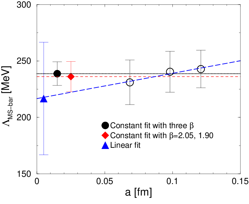
As the last step we take the continuum limit using the three lattice spacings from Ref. [1]. The scaling behavior of $\alpha_{s}(M_{Z})$ and $\Lambda_{\overline{\rm MS}}^{(5)}$ is plotted in Fig. 6. Since the results in the continuum limit do not depend on $L_{\rm max}$, we adopt the result for $L=6$ as the central value for $\beta=2.05$.

We tested three types of continuum extrapolation; a constant fit with three or two data points, or a linear extrapolation ¹¹ 1 ${\cal O}(g_{0}^{2}a/L)$ error is expected from boundary terms in temporal direction in the SF scheme, which may propagate to $\alpha_{s}(M_{Z})$ through $\overline{g}^{2}(L_{\rm max})$.. These results agree with each other and we adopt the constant fit with three data points for our final results since there is almost no scaling violation. Our final results are

where the first parenthesis is statistical error and the second is systematic error of perturbative matching of different flavors, which is estimated as a difference between results with three- and two- loop matching relation for (III.12) and may be overestimated. The last parenthesis is a difference between the constant and a linear extrapolation and is a systematic error due to finite lattice spacing for physical inputs.

We have presented a calculation of the running coupling constant for the $N_{f}=2+1$ QCD in the mass independent Schrödinger functional scheme in the chiral limit. We used seven scales to cover low to high energy regions and three lattice spacings to take the continuum limit at each scale.

After tuning $\beta$ and $\kappa$ to fix seven scales in the massless limit we evaluated the step scaling function in the continuum limit. We notice that deviation (IV.10) from the continuum SSF is rather large at one loop for our choice of the Iwasaki gauge action and the tree level improvement for boundary coefficient $c_{t}^{P/R}$. Since the one loop formula could not reproduce the numerical data except for very high $\beta\geq 10$ we adopted “two loops” formula extracted from numerical data with quadratic fit. With the “perturbative” improvement the SSF shows good scaling behavior and the continuum limit seems to be taken safely with a constant extrapolation of the finest two lattice spacings.

We notice that “two loop” term in the deviation (IV.11) has been comparable to that at one loop. There may be a possibility that higher order perturbative correction contribute in an non-negligible manner, which may introduce an unestimated systematic error. However we consider the probability is not so high since scaling behavior of the “two loops” improved SSF is good as in Fig.3 and the continuum limit was taken safely. But a further test may be preferable with a different setup with better perturbative behavior for the SSF.

With the non-perturbative renormalization group flow we are able to estimate the renormalization group invariant scale $\Lambda_{\rm QCD}$ and $\alpha_{s}(M_{Z})$ with some physical inputs for energy scale. The physical scale is introduced from the spectrum simulations of CP-PACS/JLQCD collaboration [1] through the hadron masses $m_{\pi}$, $m_{K}$, $m_{\Omega}$. From these inputs we evaluated (VI.1) and (VI.2), where all the statistical and systematic errors are included. Our result is consistent with recent lattice results [10, 11, 12, 15] and the Particle Data Group average $\alpha_{s}(M_{Z})=0.1176(20)$ [38] with the systematic error included.

For a future plan a new result is going to be available by the PACS-CS Collaboration [39, 40] aiming at simulations at the physical light quark masses down to $m_{\pi}/m_{\rho}\approx 0.2$. This may reveal a systematic error from the physical scale input due to chiral extrapolation toward light quark masses. With progress in the physical point simulation expected in the near future, we are hopeful that a full control of errors in the lattice QCD determination of the strong coupling constant is in sight.

This work is supported in part by Grants-in-Aid of the Ministry of Education, Culture, Sports, Science and Technology-Japan (Nos. 18740130, 18104005, 20340047, 20105001,20105003, 21340049).

References

• [1] T. Ishikawa et al. [JLQCD Collaboration], Phys. Rev. D 78 (2008) 011502 [arXiv:0704.1937 [hep-lat]].
• [2] G. P. Lepage and P. B. Mackenzie, Phys. Rev. D 48 (1993) 2250 [arXiv:hep-lat/9209022].
• [3] Y. Schröder, Phys. Lett. B 447 (1999) 321 [arXiv:hep-ph/9812205].
• [4] A. X. El-Khadra, G. Hockney, A. S. Kronfeld and P. B. Mackenzie, Phys. Rev. Lett. 69 (1992) 729.
• [5] G. P. Lepage and J. H. Sloan [NRQCD Collaboration], Nucl. Phys. Proc. Suppl. 34 (1994) 417 [arXiv:hep-lat/9312070].
• [6] S. Aoki et al., Phys. Rev. Lett. 74 (1995) 22 [arXiv:hep-lat/9407015].
• [7] M. Gockeler, R. Horsley, A. C. Irving, D. Pleiter, P. E. L. Rakow, G. Schierholz and H. Stuben [QCDSF Collaboration and UKQCD Collaboration], Nucl. Phys. Proc. Suppl. 140 (2005) 228 [arXiv:hep-lat/0409166].
• [8] C. T. H. Davies et al. [HPQCD Collaboration and UKQCD Collaboration and MILC Collaboration and], Phys. Rev. Lett. 92 (2004) 022001 [arXiv:hep-lat/0304004].
• [9] Q. Mason et al. [HPQCD Collaboration and UKQCD Collaboration], Phys. Rev. Lett. 95 (2005) 052002 [arXiv:hep-lat/0503005].
• [10] C. T. H. Davies, K. Hornbostel, I. D. Kendall, G. P. Lepage, C. McNeile, J. Shigemitsu and H. Trottier [HPQCD Collaboration], Phys. Rev. D 78 (2008) 114507 [arXiv:0807.1687 [hep-lat]].
• [11] C. T. H. Davies et al. [HPQCD Collaboration], arXiv:0810.3548 [hep-lat].
• [12] K. Maltman, D. Leinweber, P. Moran and A. Sternbeck, PoS LATTICE2008 (2008) 214 [arXiv:0812.2484 [hep-lat]].
• [13] P. Weisz, Nucl. Phys. Proc. Suppl. 47 (1996) 71 [arXiv:hep-lat/9511017].
• [14] P. E. L. Rakow, Nucl. Phys. Proc. Suppl. 140 (2005) 34 [arXiv:hep-lat/0411036].
• [15] I. Allison et al. [HPQCD Collaboration], Phys. Rev. D 78 (2008) 054513 [arXiv:0805.2999 [hep-lat]].
• [16] E. Shintani et al. [JLQCD Collaboration and TWQCD Collaboration], arXiv:0807.0556 [hep-lat].
• [17] M. Lüscher, R. Narayanan, P. Weisz and U. Wolff, Nucl. Phys. B 384 (1992) 168. [arXiv:hep-lat/9207009].
• [18] M. Lüscher, R. Sommer, P. Weisz and U. Wolff, Nucl. Phys. B 413 (1994) 481. [arXiv:hep-lat/9309005].
• [19] S. Sint, Nucl. Phys. B 421 (1994) 135 [arXiv:hep-lat/9312079].
• [20] S. Sint, Nucl. Phys. Proc. Suppl. 94 (2001) 79 [arXiv:hep-lat/0011081] and references there in.
• [21] M. Della Morte, R. Frezzotti, J. Heitger, J. Rolf, R. Sommer and U. Wolff [ALPHA Collaboration], Nucl. Phys. B 713 (2005) 378. [arXiv:hep-lat/0411025].
• [22] S. Takeda, S. Aoki and K. Ide, Phys. Rev. D 68 (2003) 014505. [arXiv:hep-lat/0304013].
• [23] S. Takeda et al., Phys. Rev. D 70 (2004) 074510. [arXiv:hep-lat/0408010].
• [24] K. Murano, S. Aoki, S. Takeda and Y. Taniguchi, PoS LATTICE2008 (2008) 228 [arXiv:0903.1154 [hep-lat]].
• [25] S. Aoki et al. [CP-PACS Collaboration], Phys. Rev. D 73 (2006) 034501. [arXiv:hep-lat/0508031].
• [26] S. Aoki, R. Frezzotti and P. Weisz, Nucl. Phys. B 540 (1999) 501. [arXiv:hep-lat/9808007].
• [27] A. Bode, P. Weisz and U. Wolff [ALPHA collaboration], Nucl. Phys. B 576 (2000) 517 [Erratum-ibid. B 600 (2001 ERRATA,B608,481.2001) 453]. [arXiv:hep-lat/9911018].
• [28] S. A. Larin, T. van Ritbergen and J. A. M. Vermaseren, Nucl. Phys. B 438 (1995) 278 [arXiv:hep-ph/9411260].
• [29] K. G. Chetyrkin, B. A. Kniehl and M. Steinhauser, Phys. Rev. Lett. 79 (1997) 2184 [arXiv:hep-ph/9706430].
• [30] K. G. Chetyrkin, B. A. Kniehl and M. Steinhauser, Nucl. Phys. B 510 (1998) 61 [arXiv:hep-ph/9708255].
• [31] W. Bernreuther and W. Wetzel, Nucl. Phys. B 197 (1982) 228 [Erratum-ibid. B 513 (1998) 758].
• [32] W. Bernreuther, Annals Phys. 151 (1983) 127.
• [33] G. Rodrigo and A. Santamaria, Phys. Lett. B 313 (1993) 441 [arXiv:hep-ph/9305305].
• [34] http://qcdoc.phys.columbia.edu/cps.html
• [35] T. Kaneko, S. Aoki, M. Della Morte, S. Hashimoto, R. Hoffmann and R. Sommer, JHEP 0704 (2007) 092. [arXiv:hep-lat/0703006].
• [36] S. Sint and R. Sommer, Nucl. Phys. B 465 (1996) 71. [arXiv:hep-lat/9508012].
• [37] S. Takeda, Private communication.
• [38] C. Amsler et al. (Particle Data Group), Physics Letters B667, 1 (2008) and 2009 partial update for the 2010 edition .
• [39] S. Aoki et al. [PACS-CS Collaboration], Phys. Rev. D79 (2009) 034503 [arXiv:0807.1661 [hep-lat]].
• [40] N. Ukita et al. [PACS-CS Collaboration], PoS LAT2008 (2008) 097 [arXiv:0810.0563 [hep-lat]].
β\beta κ\kappa L/aL/a g¯2​(L)\overline{g}^{2}(L) mPCACm_{\rm PCAC} 2​L/a2L/a g¯2​(2​L)\overline{g}^{2}(2L) mPCACm_{\rm PCAC}