Fixed-parameter tractability and lower bounds
for stabbing problems
Abstract
We study the following general stabbing problem from a parameterized complexity point of view: Given a set of translates of an object in , find a set of lines with the property that every object in is ”stabbed” (intersected) by at least one line.
We show that when consists of axis-parallel unit squares in the (decision) problem of stabbing with axis-parallel lines is W[1]-hard with respect to (and thus, not fixed-parameter tractable unless FPT=W[1]) while it becomes fixed-parameter tractable when the squares are disjoint. We also show that the problem of stabbing a set of disjoint unit squares in with lines of arbitrary directions is W[1]–hard with respect to . Several generalizations to other types of objects and lines with arbitrary directions are also presented. Finally, we show that deciding whether a set of unit balls in can be stabbed by one line is W[1]–hard with respect to the dimension .
Keywords: geometric stabbing, minimum enclosing cylinder, lower bounds, fixed-parameter tractability.
1 Introduction
We study several instances of the following general stabbing problem from a parameterized complexity point of view: Given a set of translates of an object in , find a set of lines with the property that every object in is ”stabbed” (intersected) by at least one line. Examples include the problem of stabbing a set of axis-parallel squares or circles in the plane with lines (possibly axis-parallel), stabbing cubes in space with planes, and stabbing unit balls in with one line (the decision version of the problem of computing the smallest enclosing cylinder).
All these problems are known to be NP-hard and for most of them only polynomial time constant-factor approximation algorithms are known up to date. We study several such problems from a parameterized complexity point of view: Our goal is to determine if algorithms that run in time on inputs of size (where is a computable function depending only on , and is a constant independent of ) do exist.
Parameterized Complexity
We first review some basic definitions of parameterized complexity theory; see [7, 8] for an introduction. A problem with input size and a positive integer parameter is fixed-parameter tractable if it can be solved by an algorithm that runs in time, where is a computable function depending only on , and is a constant independent of ; such an algorithm is (informally) said to run in fpt-time. The class of all fixed-parameter tractable problems is denoted by FPT. An infinite hierarchy of classes, the W-hierarchy, has been introduced for establishing fixed-parameter intractability. Its first level, W[1], can be thought of as the parameterized analog of NP: a parameterized problem that is hard for W[1] is not in FPT unless FPT=W[1], which is considered highly unlikely under standard complexity theoretic assumptions. Hardness is sought via an fpt-reduction, i.e., a fpt-time many-one reduction from a problem , parameterized with , to a problem , parameterized with , such that for some computable function .
Results
Our results are given by the following theorems listed in the order in which they are proved in the relevant sections.
Theorem 1.
Stabbing a set of axis-parallel unit squares in the plane with axis-parallel lines is W[1]–hard with respect to .
We prove this by an fpt-reduction from the -Clique problem in directed graphs, which is known to be W[1]-complete [8]. This main construction is modified to work for the case when the lines can have arbitrary directions, and by replacing the squares with rectangles in a proper way, we get the following theorem:
Theorem 2.
Stabbing a set of disjoint rectangles in the plane with lines is W[1]–hard with respect to , for both cases where the lines are axis-parallel or have arbitrary directions.
By simply applying a linear transformation, this leads to the following theorem, which complements the results of Langerman and Morin [12], who showed that the same problem for points is fixed parameter tractable.
Theorem 3.
Stabbing a set of disjoint unit squares in the plane with lines of arbitrary directions is W[1]–hard with respect to .
These theorems are generalized to a large class of objects (for example, squares, circles, triangles).
Theorem 4.
Let be a connected object in the plane. (i) If the stabbing lines are to be parallel to two different directions that are part of the input, the problem of stabbing a set of disjoint translates of with lines is W[1]–hard with respect to , unless is contained in a line parallel to or . (ii) The problem of stabbing a set of disjoint translates of with lines in arbitrary directions is W[1]–hard with respect to .
In contrast to the above, some special cases of the problem become fixed parameter tractable. Let be set of directions. A line with a direction from is called a -line. A set of objects with the property that the maximum number of objects that can be simultaneously intersected by two -lines with different directions is bounded by is called –shallow for . E.g., if we consider the case of axis-parallel disjoint unit squares and axis-parallel lines, the resulting sets are 1–shallow.
Theorem 5.
(i) Stabbing a set of axis-parallel disjoint unit squares with axis-parallel lines is fixed parameter tractable. (ii) The problem of stabbing a set of translates of a planar connected object that is -shallow for a set of many directions with -lines can be decided in time for every fixed .
Our algorithm is based on simple data reduction and branching rules that lead to a problem kernel.
Again on the negative side, we show the following:
Theorem 6.
Stabbing unit balls in with one line is W[1]–hard with respect to .
Note that since the balls are unit, the above problem is the decision version of the minimum enclosing cylinder problem. We prove this result by an fpt-reduction from the -independent set problem in general graphs, which is known to be W[1]-complete [8]. In the reduction, the dimension is linear in the size of the independent set, hence an -time algorithm for this problem implies an -time algorithm for the -independent set problem, which in turn implies that -variable SAT can be solved in -time. The Exponential Time Hypothesis (ETH) [11] conjectures that no such algorithm exists.
Table 1 summarizes our results in . The numbers refer to the theorems that prove the corresponding case. If no reference is given, the result is trivially implied by the result on its left side.
| axis-parallel | two dir. fixed | two dir. input | arbitrary | |
| unit squares | W[1]–h (1) | W[1]–h | W[1]–h | W[1]–h (3) |
| disj. unit sq. | FPT(5 (i)) | FPT(5 (ii)) | W[1]–h (4 (i)) | W[1]–h (3) |
| disj. rect. fixed | FPT(5 (ii)) | FPT(5 (ii)) | W[1]–h (4 (i)) | W[1]–h (4 (ii)) |
| disj. rect. input | W[1]–h (2) | W[1]–h | W[1]–h | W[1]–h (4 (ii)) |
Related Results
The parameterized complexity of geometric problems has not been studied extensively in the past. Some recent examples include work about Klee’s measure problem [5], clustering [4, 13], and shape-matching [2]. The survey by Giannopoulos et al. [9] provides an extensive overview of the known results in the area.
The problem of stabbing (or hitting) unit balls in with one line was show to be NP-hard when is part of the input by Megiddo [14]; unless P=NP, the paper also rules out the existence of a polynomial time approximation scheme for this problem. This problem is equivalent to the minimum enclosing cylinder problem for points, see Varadarajan et al. [15]. Exact and approximation algorithms for the latter problem can be found, for example, in Bădoiu et al. [1].
Langerman and Morin [12] showed that an abstract -hard covering problem that models a number of concrete geometric (as well as purely combinatorial) covering problems is in FPT. One example is the problem of deciding if a set of points in the plane can be covered (stabbed) by lines.
Hassin and Megiddo [10] showed that stabbing line segments with axis-parallel lines is NP–hard even when the segments are unit and horizontal. They also developed various constant factor approximation algorithms for stabbing sets of translates of a given object in the plane and in higher dimensions with axis-parallel lines.
Recently, and independently of our work, Dom et al. [6] considered the parameterized complexity of a stabbing problem similar to ours: Given a set of axis-parallel lines in the plane and a set of axis-parallel rectangles, find a set of of those lines that stab the rectangles. They showed that this problem is W[1]–hard (the reduction produces rectangles of different sizes). They also claim that this is true even for axis-parallel squares and that the problem is in W[1], however no proofs are given for these two results. Observe that their hardness result does not imply Theorem 1 since, while stabbing axis-parallel unit squares with axis-parallel lines (the lines are not given) obviously reduces to the problem they consider, the converse is not at all obvious. They also showed that for disjoint rectangles the problem is fixed-parameter tractable under the condition that each rectangle is stabbed by the same number of vertical and horizontal lines in the given set.
2 Stabbing with lines
2.1 Hardness Results
In this section we present the hardness results. The proofs are by a reduction from the –Clique problem for directed graphs, which is shown to be W[1]–complete in [7]. First, in Section 2.1.1, we show that the problem of stabbing axis-parallel unit squares with axis-parallel lines is W[1]–hard. This construction is then modified to work for the case when the lines can have arbitrary directions. From this, minor modifications are made to prove that for this case, the problem is even hard when the squares are disjoint. Finally, we show that the proofs also work for a large class of other objects. In this section, the objects are assumed to be open, but it is easy to modify the proofs to work for closed objects, too.
2.1.1 Stabbing axis-parallel unit squares with axis-parallel lines in the plane
From a given graph we will construct a set of axis-parallel unit squares in that can be stabbed by lines if and only if the graph has a –clique. The set will be of size and thus polynomial in both and .
General Idea
Let and be a simple directed graph with no loops. For clarity of presentation, we first create instances that consist of squares of two different sizes, namely some with side length and some with side length . A minor modification will then make them all have the same size.
As all the squares placed in have integer coordinates and are open, we can simplify our arguments using the following two observations:
Observation 1:
All the lines of the form or for can be neglected, as they can be replaced by any line of the form or , , respectively, without intersecting fewer squares.
and
Observation 2: Two lines , with , , intersect the same squares, and analogously for vertical lines.
In the final construction there will be horizontal and vertical double strips, and , respectively, to choose lines from. Out of each of those strips, two “consistent” lines will have to be chosen in order to get a solution of the specified size. Around every intersection of two such orthogonal strips, we will place a gadget, consisting of a set of squares, within a region of suitable size, as indicated in Figure 1.
We will ensure that any selection of such lines has the following properties
- :
Each two lines inside the same double strip will correspond to the same vertex.
- :
Two orthogonal line pairs in the strips , , will stab all the squares inside the region if and only if they represent vertices that are connected in .
- :
Two orthogonal line pairs in the strips will stab all the squares inside the region if and only if they correspond to the same vertex.
Any selection of such line pairs will then correspond to a set of vertices and will stab all the squares if and only if the vertices in form a –clique in .
Besides these lines, we will need more lines to guarantee the consistency of such a selection (). To ensure the properties, several gadgets are constructed, which we will describe in detail now.
The Gadgets
In the following, let denote the axis-parallel square with side length and lower left corner . A gadget will consist of a collection of axis-parallel squares. Let denote the copy of whose squares are placed relative to . We say that a square is at position in gadget , if the lower left corner of the square has absolute coordinates . Unless stated otherwise, the coordinates of axis-parallel lines are also given relative to the gadget’s offset, i.e., if we refer to lines and passing through the gadget , we speak about the lines and , respectively.
The –Gadget (Forcing)
The –gadget will be used to ensure that in any solution of size , a line through a specified strip (of width ) must be chosen. We define them as
and
The fact that they really force lines in the specified region follows from the very simple
Proposition 7.
In order to stab a gadget by lines, at least one line of the form (relative to the gadget) for some must be chosen.
For reasons of symmetry, an analogous proposition holds for the vertical case as well. We now define the correspondence of lines chosen to vertices in :
Definition 8.
A line through a horizontal –gadget is said to represent vertex , and analogously for the vertical case.
As the –gadgets have a width of , for each vertex in there exists a line that represents this vertex. Because of Observation 2, two lines that represent the same vertex in a gadget will intersect the same squares. The (open) strips of width 1 where all the lines represent the same vertex are called v(ertex)–strips. Each double strip (of width ) will consist of vertex strips. See Figure 2.
The –Gadget (Adjacency)
This gadget represents the adjacency relation of the graph . All the squares will be placed inside a region of size . For each pair of vertices such that , including the missing loops , it will contain a square that forbids the line pairs corresponding to these vertices to be chosen at the same time, namely .
So
In the final construction, there will be four –gadgets forcing one line through each of the strips
- •
- •
- •
- •
relative to the gadget’s coordinates. and define a horizontal and and a vertical double strip.
If a line lies inside or , it is called negative, otherwise it is called positive. Two parallel lines are called antipodal if one is negative and the other is positive. In the final construction, it will be ensured that if a negative line is chosen that represents vertex , then, in the same double strip, a parallel positive line must be chosen that also represents . Such a line pair is then said to represent vertex .
The main property of the –gadget is stated by the next lemma.
Lemma 9.
Two antipodal vertical lines through that both represent and two antipodal horizontal lines through that both represent intersect all the squares inside if and only if .
Proof.
If a square is not intersected by these lines, we must have and and thus . If, conversely, , then the square is in but is not intersected by any of these four lines. ∎
With this it will be possible to ensure property . Observe that, as the graph contains no loops, also is ensured.
An example is shown in Figure 3. There, the directed edges in both directions are drawn as a single undirected edge. The four squares added for the missing loops are not shown.
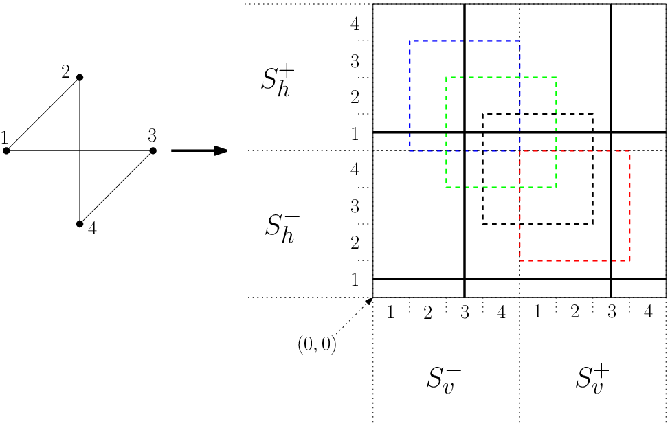
The –Gadget (Diagonal)
This gadget is a special –gadget for the graph with the adjacency defined by the identity matrix . It thus consists of the squares
and will be used to ensure property . The regions forced through such a gadget will be the same as for the –gadgets. Thus, by applying Lemma 9, all the squares inside a –gadget are stabbed if and only if the vertical and the horizontal antipodal line pair represent the same vertex.
The –gadget (Consistency)
This type of gadget will guarantee a certain distance between two antipodal lines of the same direction inside the same double strip.
It ensures that if a size solution contains a negative line that represents vertex , then, in the same double strip, it also contains a positive parallel line that represents the same vertex. Thereby it will be possible to identify such a line pair with the vertex , which will ensure property .
We continue to describe the –gadgets for the horizontal case. A –gadget consists of the union of the two sets
and
In the final construction there will be three –gadgets that ensure the existence of a line in each of the strips
- •
- •
- •
relative to the placement of the gadget. So, in any solution of size , through each –gadget there will be three lines. Why two of them are given the same name as the strips for the –gadgets will become clear soon.
As for an –gadget, there are again combinatorially different horizontal strips to chose lines from. The following lemma states the main property of the –gadgets:
Lemma 10.
Let be two antipodal horizontal lines in , respectively, then there exists a vertical line that together with intersects all of the squares belonging to the –gadget if and only if .
Proof.
First suppose . Then the two squares and are defined and are both not stabbed by these two lines. But as
they cannot be stabbed by a single vertical line (recall that the squares are open). See Figure 5.
If, conversely, (if either or , it is trivial), we have that
as
i. e., the left side of every –square that is not stabbed is to the left of the right side of every –square that is not stabbed. Thus, all the squares left can be stabbed by a single vertical line, namely any line of the form for . See Figure 5. ∎

In particular, all squares in a –gadget are intersected if the three lines in all represent the same vertex.
For the sake of completeness, we give the exact coordinates of the –gadgets:
The Construction
We now come to describe the exact placement of the gadgets. The main part, expressing the adjacency relation of the graph, will be a grid of – and –gadgets:
Around this grid, we add the –gadgets to allow only specific solutions:
Here it becomes clear why we chose the coordinates as multiples of : The –gadgets now cannot influence each other, i.e., no square from one such gadget intersects any strip belonging to another –gadget.
Finally, we place the –gadgets to force lines in the desired strips as follows: For the double strips, the lines are forced by
and
The additional lines for the –gadgets are forced by
and
The entire construction is shown in Figure 6, where the three regions belonging to are indicated.
The set
is of size and takes time polynomial in both and to create.
It has the following property:
Lemma 11.
can be stabbed by axis-parallel lines if and only if has a –clique.
Proof.
Observe that the horizontal as well as the vertical –gadgets are pairwise disjoint, so by Lemma 7, at least one line in the corresponding direction is needed for each of them. Thus, in any solution there have to be at least lines.
Let have a –clique . First, we choose lines as follows: For , we choose the line pairs (horizontal) and (vertical) in the strips and , respectively, such that they are antipodal and correspond to the vertex .
Then we have, for parallel lines, that () and thus we can apply Lemma 10, i. e., the squares left in the –gadgets can be intersected by additional lines. By Lemma 9, all the squares inside are intersected, as for all . Further, as and represent the same vertices, all –gadgets are also stabbed. Thus, lines suffice.
Now assume that the set can be stabbed by axis-parallel lines. Because of the
–gadgets, through each – and –gadget there must be exactly
two antipodal horizontal and two antipodal vertical lines. Also, through each –gadget there are exactly three lines, two of which are parallel.
Further, by Lemma 10 we have for each such antipodal pair of lines in the same double strip that ,
for otherwise the corresponding –gadget would not be stabbed. We can
assume that for all : enlarging the gap between the two antipodal parallel
lines can only reduce the set of squares that are intersected in the – and –gadgets, and, by Lemma 10, the additional line in the gadgets can then be chosen to represent , too. Each such pair of lines thus corresponds
to a node in (). Let be the nodes
represented by the horizontal line pairs and
the nodes represented by the vertical line pairs. By Lemma 9, the gadget ensures that for all (), and thus we have . Further, the gadget
ensures that for all (), which also
implies for all as the graph contains no loops. But this means that forms a –clique in .
∎
Adaption to Unit Squares
To make all the squares have a side length of , we simply shrink the squares inside the –gadgets by from each side, i. e. we redefine the –gadgets as
- •
and
- •
.
and define accordingly. The only lines influenced by this are the ones that represent either or . Because all the lines that represent in a gadget intersect the same squares in , we can assume that any such line in a solution is of the form . The same argument holds for the lines that represent , i. e., they can assumed to be of the form ; again, the same holds analogously for vertical lines. Thus, if there is a solution of size for , then there is also one for . This completes the proof of Thm. 1.
2.1.2 Arbitrary directions
So far our results depended on the lines being parallel to the coordinate axis. In this section, starting with the set of axis-parallel unit squares from section 2.1.1, we show how to modify this construction to yield a set of axis-parallel unit squares that works for the case where the lines can lie in arbitrary directions. Observe that, while intuitively plausible, it is not a priori clear that this problem is also W[1]–hard just because the problem for axis-parallel lines is hard.
The proof that this problem is hard is more technical than above, even though the idea remains the same. The main task will be to modify the set in such a way that the lines in any solution must be “almost” axis–parallel. This will be done by increasing the number of squares the –gadgets and shrinking the squares a little. With this it will be possible to show that all the almost axis-parallel lines have an equivalent axis-parallel line.
To make calculations easier, we first modify by applying the linear function that scales in – and –direction by . If we now refer to , we mean the scaled set. All the squares in this set have side length . The vertex–strips for then have a width of , and the vertex–strips for and have a width of .
Shrinking the Squares
To shrink a square by means that we replace a square by , i.e., shrink it from each side by a value of . We begin with the definition of –robustness which will prove to be very useful in the following argumentation.
Definition 12.
A set of squares is called –robust, if
for .
A set that is –robust can be altered a little without “destroying” any solutions. The following lemma will be used in its full strength in the next section. During this section, we will only consider modifications that shrink the squares.
Lemma 13.
Let be a –robust set of axis-parallel unit squares that can be stabbed by axis-parallel lines. If we translate each square by a value at most and shrink each square by a value such that , then the resulting set still can be stabbed by axis-parallel lines. Further, if all the squares are shrinked by (and not translated), then the resulting set is –robust.
Proof.
For a set , let denote the modified set. Obviously, for any set of squares we have , , if and only if there exists an axis-parallel line that stabs all squares from . We show that the modified set still lies on a common axis-parallel line. Let be horizontal and
The line intersects all the squares from . Further, , as the set is –robust. Thus, after shrinking and translating the squares in by a value of at most and , respectively, for the corresponding values of the modified set we still have
Thus, stabs all the squares from . Again, the same argument works for vertical lines as well.
To prove the second part, observe that
for
∎
See Figure 7.
(Observe that in general the reverse is not true.)
We will now modify the set to yield a set in two steps as follows:
- 1.
The –gadgets are enlarged to now contain squares, i.e. we set
and
(Recall that we have scaled the set by to contain squares of length ).
- 2.
In the resulting set, all the squares are shrinked by .
The resulting set then consists of unit squares with side length . We will make use of the following observation, which is easy to check:
Observation 1: For any two squares from and , we have that
That means that if two squares cannot be interesected by, e.g., a common vertical line, then there is a horizontal distance of at least between them. Lemma 13 is used to prove the following property of our set :
Lemma 14.
The set can be stabbed by axis-parallel lines if and only if can be stabbed by axis-parallel lines.
Proof.
First observe that if we are only considering solutions of size with axis-parallel lines, then it does not matter whether the –gadgets consist of or squares.
“”: The squares from all contain a square from , thus any solution to is a solution to .
“”: By the construction of , it is –robust and . Thus, we can apply Lemma 13.
∎
By we denote the modified version of gadget , e. g., is the –gadget with the squares shrinked as described above. The following proposition is used to show that in any solution of size the lines have to be almost parallel to the axis.
Proposition 15.
A line can intersect at most squares of a single gadget and at most of a single –gadget.
Proof.
For any two points and where the line stabs a square from an –gadget, we must have , which means and thus . Thus, as the squares inside the –gadget are all disjoint, at most of them can be stabbed by such a line. Rotation by 90 degrees shows that for the –gadgets at most squares can be stabbed.
∎
To prove the main property of the lines, we first only consider the set of –gadget and do not add the –, –, and –gadgets yet.
As all the squares in are placed between , , , and , it suffices to consider the behaviour of the lines inside the region . Then the following holds:
Lemma 16.
In order to stab the –gadgets with lines in arbitrary directions, each of the lines has to intersect a single –gadget entirely.
Proof.
It suffices to show that any line can stab at most squares and that this is the case only if it stabs a single –gadget entirely. As there are squares to stab, the claim follows. Without loss of generality, let for some ; the vertical case is symmetric. We call such a line that stabs squares an –line and show in three steps:
- a.
An –line must have a slope .
- b.
An –line cannot intersect squares from two different –gadgets.
- c.
An –line cannot intersect any squares from an –gadget.
from which it follows that an –line must intersect a single entire –gadget.
a. If the slope is larger than , i. e., , by Proposition 15 the line can stab at most
squares. So any –line must have a slope .
b. When such a line intersects a square of one –gadget at , it cannot intersect any square of another –gadget at unless (the gap between two –disjoint squares, see Observation 1) and thus (as ). In particular, if such a line intersects the –th square (from the right) of one –gadget, it cannot intersect the –th square from another –gadget for .
Let denote the number of different –gadgets intersected. Then the total number of squares stabbed is at most , which is less than for . Thus we have , i. e. any –line can intersect at most one –gadget and must stab at least of its squares. Thus it must have a slope of at most .
c. In order for a line to stab squares of a single –gadget, it must intersect the –th square (from the right) of this gadget. Thus, at , any –line must be above , which is below the lowest point where it can stab any square from an –gadget. (Observe that the bounds are even stronger, e.g., any such line must even be above , but this is not needed here). Then the line cannot stab any square from an –gadget, as
and any square from an –gadget lies below . So it must lie entirely inside a single –gadget in order to be an –line. Analogous calculations prove the same for the case when the line is almost vertical. ∎
Figure 8 indicates the coordinates used.

Thus, for the gadgets only, we know that in order to stab all the squares with lines, one line must intersect exactly one (entire) –gadget. In order to do so, by Proposition 15, it must have a slope of at most (in the horizontal case) or at least (in the vertical case). The crucial point is that if we now add squares to the existing set, these properties remain.
The Final Construction
Now we place the remaining squares from . Recall tha, by Lemma 14, can be stabbed by axis-parallel lines iff can be stabbed by axis-parallel lines.
By shrinking, we have created a small “fuzzy” region (see Observation 1) and have thereby achieved that the small change that a line can make after leaving its –gadget cannot influence the solution. This is expressed by the next lemma:
Lemma 17.
In any solution to with arbitrary lines, without loss of generality the lines can assumed to be axis–parallel, i. e., if there is a solution with arbitrary lines, then there is also one with axis-parallel lines.
Proof.
Let be an almost horizontal line with slope . As the line has to intersect an entire –gadget, it suffices to calculate the change it can make between the minimum –position where it can leave an –gadget, namely (Figure 8), and , which is
Thus, it cannot intersect any two –disjoint squares, from which it follows that it can be replaced by a horizontal line. Again, similar calculations prove the vertical case. ∎
That means if there is a solution with arbitrary lines for the set , then there is also one where all the lines are axis–parallel. Using Lemma 14, it follows that can be stabbed by axis-parallel lines if and only if can be stabbed by arbitrary lines, which proves the following:
Theorem 18.
Stabbing a set of axis-parallel unit squares in the plane with lines of arbitrary directions is W[1]–hard with respect to .
2.1.3 Sets of disjoint objects
In this section we show that some of the problems are even hard for sets of disjoint objects. First, we show that stabbing disjoint rectangles with axis-parallel lines is W[1]–hard if the rectangles can be chosen arbitrarily. This goes by a small modification of the sets in the previous sections. It is important to notice that for this problem, the rectangle chosen for the reduction, i.e., the ratio of its side lengths, depends on , in contrast to the results in the previous section, where (after scaling the construction) only a single base object was required.
From this we derive, as a main result, that stabbing disjoint axis-parallel unit squares with lines in arbitrary directions is also W[1]–hard, in contrast to the case where the lines have to be axis–parallel, which is covered in the next chapter.
The proof will consists of three steps which we will sketch here first:
- 1.
“Wobble” the squares in a little, such that all the (parallel) diagonals of the squares are disjoint.
- 2.
Replace each diagonal with a very thin rectangle, such that all the resulting rectangles are disjoint.
- 3.
Transform the set of rectangles to a set of unit squares via a bijective linear transformation.
2.1.4 Disjoint Rectangles
Starting with the set from the previous section, we will construct a set of disjoint rectangles that can be stabbed by lines if and only if the can. This will prove the hardness for both the cases where the lines chosen have to be axis-parallel as well as for arbitrary lines.
Recall that the squares in have a side length of for the defined as . By Lemma 17, the set can be stabbed by arbitrary lines if and only if it can be stabbed by axis-parallel lines, and by Lemma 13, the set is –robust, as is –robust and .
We will modify the set such that no two (parallel) diagonals intersect any more while maintaining the significant combinatorial properties. Recall that right now for an –, –, and –gadgets, the diagonals of some of the squares may intersect, as indicated in Figure 9.

Let and . The new squares will have a side length of . We define the wobble–function , which shrinks and translates the squares, as follows:
We now take the set and wobble the squares inside the –, , and –gadgets. For the – and –gadgets, we apply to the square that is added for (which is , relative to the gadget’s offset).
Each –gadget contains squares. For each such gadget, we apply to the –th square. The other squares, i. e., those contained in the –gadgets, are simply shrinked (but not shifted) to be all of size . This yields a set of axis-parallel unit squares .
Now we want replace the diagonals of the squares in by very thin rectangles, which will be all disjoint. We define the rectangle by its endpoints
as shown in Figure 10.
Instead of each square in we now place a rectangle whose bounding box is this square.
Thereby we have achieved that all the rectangles created (which are all copies of ) are disjoint, as the distance of two diagonals is now at least . Thus, the resulting set is a set of disjoint translates of .
Now we can show the main lemma of this section, which completes the proof of Thm. 2.
Lemma 19.
can be stabbed by lines if and only if can be stabbed by lines.
Proof.
We prove that the following are equivalent
- (i)
can be stabbed by arbitrary lines.
- (ii)
can be stabbed by axis-parallel lines.
- (iii)
can be stabbed by axis-parallel lines.
- (iv)
can be stabbed by arbitrary lines.
(i) (ii): By Lemma 17.
(ii) (iii): Obviously, an axis-parallel line intersects a square iff and only if it intersects its inscribed rectangle . As the set is –robust and
we can apply Lemma 13.
(iii) (iv): trivial
(iv) (i): All the wobbled squares are contained in the original squares, as the maximum shift is and they are shrinked by from each side. Thus, any solution to the set of inscribed rectangles is also a solution to .
∎
2.1.5 Disjoint Unit Squares
To prove the case of disjoint unit squares now is an easy task. The matrix
represents a bijective linear transformation and the image of under is an axis-parallel unit square. Thus, the set consists of disjoint unit squares and is combinatorially equivalent to . This leads to the proof of Thm. 3. Also, observe that because of Lemma 19, can be stabbed by lines in direction either or , where denotes the canonical base vector, if and only if it can be stabbed by arbitrary lines. This will be used for the proof of Thm. 4 in the next section.
2.1.6 Other objects
Using the results from the previous sections, we now come prove the W[1]–hardness for a wide range of stabbing problems. The objects we will consider are those which, from two directions, “look like a square”. This can be formalized as follows:
Definition 20.
Let be two linearly independent vectors. An object is said to be a quasi–square with respect to and , if the projection of on each of the orthogonal complements of and is an open line segment, i. e., is homeomorphic to .
For an object , we define the axis-parallel bounding box as
Obviously, if and are connected, an axis-parallel line intersects the bounding box of an object if and only if it intersects the object itself.
If we are given a quasi–square with respect to and , we can transform it via the bijective linear transformation
to yield an objects that is combinatorially equivalent to a unit square when only axis-parallel lines are considered (here, denote the lengths of the projections to the orthogonal complements of and , respectively). The bounding box of then is a square with side length . Also, the image of each line parallel to or is axis–parallel As the transformation is bijective, we have
Proposition 21.
If is a quasi–square with respect to , for any –line it holds that
Thus, each instance with translates of and directions is combinatorially equivalent to an instance with unit squares and axis-parallel lines, and vice versa.
For connected objects that are not a point, also the constructions for the disjoint cases can easily be adapted: Thereto, we simply scale and rotate via a bijective linear transformation to fit inside , the rectangle described in the previous section, such that it combinatorially is “almost” the same as . Then placing such transforms of instead of in the set and applying the inverse transformation again gives a set of disjoint translates of that can be stabbed by arbitrary lines if and only if can be stabbed by arbitrary lines. We omit the technical details. See Figure 11.
Using the remark at the end of the previous section, this proves Thm. 4 (i) and (ii).
2.2 Fixed Parameter Tractable Cases
In this section, we will consider several restricted versions of the above problems that are fixed parameter tractable. Here, all the objects are assumed to be closed, but again it is easy to modify the proofs to handle open objects as well.
2.2.1 Stabbing disjoint axis-parallel unit squares with axis-parallel lines in the plane
To illustrate the idea, we first analyze the simplest case where the objects to be stabbed are disjoint axis-parallel unit squares and the lines have to be axis–parallel.
Let be such a set of unit squares. Clearly it suffices to consider only lines that support the boundary of a square in , so the total number of these relevant lines is . Let denote the set of squares in that are stabbed by . A line is said to dominate another line , if .
The following data reduction rule is required for our algorithm to work:
DR: For all squares with the same –coordinates, delete all but of them, and the same for squares that have the same –coordinates.
This rule is correct, i. e., the new set can be stabbed by lines if and only if the old one can: If there is a solution of size for the reduced set, then a solution of size for this set must contain a line that intersects all of those squares, for otherwise we would need at least lines. But any such line stabs all the deleted squares, too.
A set on which this data reduction rule is applied will be called a DR–set. The following lemma states the main idea behind the algorithm:
Lemma 22.
Let be a horizontal line that intersects unit squares . Then in order to stab the set with lines, there has to be a horizontal line that intersects at least two squares from . Further, can be chosen from the set
Proof.
There must be a line that intersects at least two of the squares because of the pigeonhole principle. This line cannot be vertical, as all of the squares are disjoint, i. e., no two of them can lie on both a common vertical and horizontal line.
We show that any such line is dominated by a line in . Let , ordered from top to bottom, and let be any line that intersects exactly the squares from (and possibly others that are not in ). Observe that always either or , as all squares have unit size. If both and , then stabs all the squares at once and is thus dominated by either or . If (the other case is symmetric) then no square that lies strictly above , i. e. is not in but intersected by , can have its upper side between and , as . Thus we have . See Figure 12.

∎
For reasons of symmetry, an analogous lemma holds for the vertical lines as well. To prove that the algorithm is correct, we need another
Lemma 23.
Let be a DR–set. If there is an axis-parallel line with , then there is also a line parallel to with .
Proof.
Let be horizontal. Since is a DR–set, the first relevant line above intersects at least squares. In general, for two neighbouring relevant lines we have that . Further, the topmost relevant line stabs at most squares, thus there must be a line in between with . ∎
We now come to describe the algorithm STAB(, ). In each call, it will find a line that stabs many () but not too many () squares, if such a line exists, and otherwise use brute force.
The SOLVE function simply counts if there are more than squares left and rejects in this case. Otherwise, it uses brute force by trying all –subsets of the at most relevant lines.
Lemma 24.
The algorithm accepts if and only if the set can be stabbed by axis-parallel lines.
Proof.
“”: Clearly, if the algorithm accepts, the set can be stabbed by lines.
“”: If there exists a line that intersects more than squares, then by Lemma 23 there is a line with . By Lemma 22, in any solution of size there must be a line that intersects at least two squares from . Further, any such line is dominated by a line in , and thus, if the set can be stabbed by lines, at least one of the branches ends up with an instance that can be stabbed by lines.
Otherwise, as mentioned above, we end up with an instance with at most squares left (otherwise we reject), and thus a solution can be found in fpt–time by the brute force algorithm.
∎
Thus, the algorithm is correct. To roughly determine the running time (a more sophisticated analysis will be given in the next section), observe that each call of the STAB function takes time , if we simply calculate all the , and branches on at most lines. Each of the branches ends up with a small instance which can be solved in steps, so the total running time is . The algorithm runs in quadratic time for every fixed and thus is an fpt–algorithm. This completes the proof of Thm. 5 (i).
2.2.2 Generalization
A closer look on the above algorithm reveals that it really only depends on two properties of the set to be stabbed:
- •
The squares are of unit size.
- •
A “large” set of squares that lie on a line in one direction cannot be intersected by “few” lines from another direction.
We will formalize these ideas and show how they can be generalized to work for different objects as well as for more than two directions. Thereto, let be a fixed set of directions. For a positive integer , a set of objects is called –shallow with respect to , if for any two –lines , it holds that
E.g., sets of disjoint unit squares with the property that each point lies in at most squares are –shallow with respect to axis-parallel lines. Also, for a fixed rectangle , sets of disjoint translates of are –shallow with respect to axis-parallel lines. We show that the problem of stabbing –shallow sets of objects that are translates of a connected object is fixed parameter tractable.
Let , where the are lines, and be a connected object. Observe that it again suffices to consider the relevant lines that support the boundary of an object.
Given a –shallow set of objects with respect to , we first apply a generalized version of the above data reduction rule:
DR’:
Given objects such that any line in direction intersects either all of them or none, delete all but of them.
This data reduction rule is correct, as in the new set there must be a line that intersects of the squares at the same time, and any such line intersects all the objects.
For two parallel lines , , we define
As the objects are closed, the functions
and
are defined. Again, we can bound the number of lines to chose from:
Lemma 25.
Let be a line in direction that intersects objects. Then in any solution of size there must be a line parallel to intersecting at least of the objects. This line can be chosen from the set
Proof.
By rotating the entire set we can assume that is horizontal. Because of the pigeonhole principle there must be a line intersecting at least objects. No line not parallel to can intersect more than of the objects, for otherwise the set would not be –shallow, thus in any solution of size there must be a line parallel to . As the objects are all of the same size, by the same arguing as in Lemma 22, any such line is dominated by a line from . ∎
Also, similar to the above reasoning, if there exists a line for a DR’–set that intersects more than objects, there must also be a parallel line with . Thus, we can simply adapt the algorithm to the new bounds. We now apply, in each call of the STAB function, the new data recuction rule DR’, and find a line with , if it exists. Lemma 25 ensures that it suffices to branch on the lines in . Thus, this algorithm accepts if and only if the set can be stabbed by –lines.
2.3 Running Time Analysis
To analyze the running time, we split the algorithm into its three main steps and calculate them independently.
Data Reduction.
The data reduction step can be done in time : First, we pick one of the directions and sort the objects according to this direction. Then we go through the array and delete all but out of each have the same coordinates according to the direction (this takes only linear time). After that, we proceed with the next direction.
Call of the STAB–procedure.
To find a line that stabs the desired number of objects, we again first pick one of the directions and sort the objects according to this direction. As they are connected, each of the objects implies two lines in each direction. For all of the lines we then calculate whether . This requires time by using binary search. As we have to do this at most times, it takes steps in total.
Solving the Problem Kernel.
Let be the number of objects left. We reject the kernel if , as no line stabs more than of them. Otherwise we can, instead of trying all of the subsets of size , use the following observation. Let be the set of relevant lines through object . By double–counting we get that
which yields , and such an objects can be found in time . Through any object there must be at least one line, so by branching on all the lines a solution is found if it exists. Thus, the kernel can be solved in time .
Total Running Time.
The algorithm branches on at most possibilities at most times, each step takes , thus the total running time is
Thereby we have shown Thm. 5 (ii).
3 Stabbing balls with one line
We show that the problem of stabbing unit balls in with a line is W[1]-hard with respect to by an fpt-reduction from the W[1]-complete -independent set problem is general graphs [7]. The reduction is based on a technique by Cabello et al. [4, 3]. Given an undirected graph we construct a set of balls of equal radius in such that can be stabbed by a line if and only if has an independent set of size . First, we construct of a scaffolding set of balls that restricts the solutions to combinatorially different solutions, which can be interpreted as potential -independent sets. Additional constraint balls will then encode the edges of the input graph.
The geometry of the construction will be described as if exact square roots and expressions of the form were available. To make the reduction suitable for the Turing machine model, the data must be perturbed using fixed-precision roundings. This can be done with polynomially many bits in a way similar to the rounding procedure followed in [4, 3]. (We omit these technical details here).
Preliminaries.
For every ball we will also have . This allows us to restrict our attention to lines through the origin: a line that stabs can be translated so that it goes through the origin and still stabs . In this section, by a line we always mean a line through the origin. For a line , let be its unit direction vector. The notions of a point and vector will be used interchangeably.
It will be convenient to view as the product of orthogonal planes , where each has coordinate axes . The origin is denoted by . The coordinates of a point are denoted by . We denote by the unit circle on centered at .
3.1 Scaffolding ball set
For each plane , we define -dimensional balls, whose centers are regularly spaced on the circle . Let be the center of the ball , , with
We define the scaffolding ball set . We have . All balls in will have the same radius , to be defined later.
Two antipodal balls , are stabbed by the same set of lines. A line stabs a ball of radius and center if and only if . Thus, stabs if and only if it satisfies the following system of inequalities:
Consider the inequality asserting that stabs . Geometrically, it amounts to saying that the projection of on the plane lies in one of the half-planes
Consider the situation on a plane . Looking at all half-planes , we see that stabs all balls (centered on ) if and and only if lies in one of the wedges ; see Fig. 13.
The apices of the wedges are regularly spaced on a circle of radius , and define the set
For to stab all balls , we must have that . We choose in order to obtain .
Since the above hold for every plane , and since is a unit vector, we have
Hence, equality holds throughout, which implies that , for every . Hence, for line to stab all balls in , every projection must be one of the apices in . Each projection can be chosen independently. There are choices, but since and correspond to the same line, the total number of lines that stab is .
For a tuple , we will denote by the stabbing line with direction vector
Two lines and are said to be equivalent if , for all . This relation defines equivalence classes , with , where each class consists of lines.
From the discussion above, it is clear that there is a bijection between the possible equivalence classes of lines that stab and .
3.2 Constraint balls
We continue the construction of the ball set by showing how to encode the structure of . For each pair of distinct indices () and for each pair of (possibly equal) vertices , we define a constraint set of balls with the property that (all lines in) all classes stab except those with and . The centers of the balls in lie in the -space . Observe that all lines in a particular class project onto only two lines on . We use a ball (to be defined shortly) of radius that is stabbed by all lines except those with and . Similarly, we use a ball that is stabbed by all lines except those with and , where . Our constraint set consists then of the four balls
We describe now the placement of a ball . Consider a line with and . The center of will lie on a line that is orthogonal to , but not orthogonal to any line with or . We choose the direction of as follows:
where , , and . It is straightforward to check that .
Let be the angle between and . We have the following lemma:
Lemma 26.
For any line , with or the angle between and satisfies .
Proof.
Without loss of generality we consider a fixed direction where (i. e., ). Consider with , , , and , where and , with and . After straightforward calculations we have that , where
We will show that . We will use the inequality:
which holds for all , with , , and . We examine the following cases:
(i) and . Then can take any value. We have
(ii) . Then . If also , we have
If , then .
(iii) . Then . The two cases where or are dealt with similarly to the previous case. ∎
This lower bound on helps us place sufficiently close to the origin so that it is still intersected by , i. e., lies in one of the half-spaces or , .
We claim that any point on with will do. For any position of on with , we have , i. e., does not stab . On the other hand, as argued above we need that . Since , we have the condition . By Lemma 26 we know that , hence by choosing so that we are done.
Reduction.
Similarly to [4], the structure of the input graph can now be represented as follows. We add to the balls in , to ensure that all components in a solution (class of lines ) are distinct. For each edge we also add the balls in sets , with . This ensures that the remaining classes of lines represent independent sets of size . In total, the edges are represented by the balls in . The final set has balls.
As noted in above, there is a bijection between the possible equivalence classes of lines that stab and the tuples . The constraint sets of balls exclude tuples with two equal indices or with indices , when , thus, the classes of lines that stab represent exactly the independent sets of . Thus, we have the following:
Lemma 27.
Set can be stabbed by a line if an only if has an independent set of size .
From this lemma and since this is an fpt-reduction, Theorem 6 follows.
References
- [1] M. Bădoiu, S. Har-Peled, and P. Indyk. Approximate clustering via core-sets. In Proc. 34th Annual ACM Symposium on Theory of Computing, pages 250–257, 2002.
- [2] S. Cabello, P. Giannopoulos, and C. Knauer. On the parameterized complexity of -dimensional point set pattern matching. In Proc. of the 2nd Int. Workshop on Parameterized and Exact Computation (IWPEC), volume 4169 of LNCS, pages 175–183, 2006.
- [3] S. Cabello, P. Giannopoulos, C. Knauer, D. Marx, and G. Rote. Geometric clustering: fixed-parameter tractability and lower bounds with respect to the dimension. ACM Transactions on Algorithms, 2009. to appear.
- [4] S. Cabello, P. Giannopoulos, C. Knauer, and G. Rote. Geometric clustering: fixed-parameter tractability and lower bounds with respect to the dimension. In Proc. 19th Ann. ACM-SIAM Sympos. Discrete Algorithms (SODA), pages 836–843, 2008.
- [5] T. M. Chan. A (slightly) faster algorithm for Klee’s measure problem. In SCG ’08: Proceedings of the twenty-fourth annual symposium on Computational geometry, pages 94–100, New York, NY, USA, 2008. ACM.
- [6] M. Dom, M. R. Fellows, and F. A. Rosamond. Parameterized complexity of stabbing rectangles and squares in the plane. In WALCOM ’09: Proceedings of the 3rd International Workshop on Algorithms and Computation, pages 298–309, Berlin, Heidelberg, 2009. Springer-Verlag.
- [7] R. G. Downey and M. R. Fellows. Parameterized Complexity (Monographs in Computer Science). Springer, November 1999.
- [8] J. Flum and M. Grohe. Parameterized Complexity Theory. Texts in Theoretical Computer Science. An EATCS Series. Springer, 1 edition, March 2006.
- [9] P. Giannopoulos, C. Knauer, and S. Whitesides. Parameterized complexity of geometric problems. Comput. J., 51(3):372–384, 2008.
- [10] R. Hassin and N. Megiddo. Approximation algorithms for hitting objects with straight lines. Discrete Applied Mathematics, 30:29–42, 1991.
- [11] R. Impagliazzo and R. Paturi. On the complexity of k-sat. J. Comput. Syst. Sci., 62(2):367–375, 2001.
- [12] S. Langerman and P. Morin. Covering things with things. Discrete & Computational Geometry, 33(4):717–729, 2005.
- [13] D. Marx. Efficient approximation schemes for geometric problems? In Proceedings of 13th Annual European Symposium on Algorithms (ESA 2005), pages 448–459, 2005.
- [14] N. Megiddo. On the complexity of some geometric problems in unbounded dimension. J. Symb. Comput, 10:327–334, 1990.
- [15] K. Varadarajan, S. Venkatesh, Y. Ye, and J. Zhang. Approximating the radii of point sets. SIAM J. Comput., 36(6):1764–1776, 2007.