Numerical determination of the exponents controlling the relationship between time, length and temperature in glass-forming liquids
Abstract
There is a certain consensus that the very fast growth of the relaxation time occurring in glass-forming liquids on lowering the temperature must be due to the thermally activated rearrangement of correlated regions of growing size. Even though measuring the size of these regions has defied scientists for a while, there is indeed recent evidence of a growing correlation length in glass-formers. If we use Arrhenius law and make the mild assumption that the free-energy barrier to rearrangement scales as some power of the size of the correlated regions, we obtain a relationship between time and length, . According to both the Adam-Gibbs and the Random First Order theory the correlation length grows as , even though the two theories disagree on the value of . Therefore, the super-Arrhenius growth of the relaxation time with the temperature is regulated by the two exponents and through the relationship . Despite a few theoretical speculations, up to now there has been no experimental determination of these two exponents. Here we measure them numerically in a model glass-former, finding and . Surprisingly, even though the values we found disagree with most previous theoretical suggestions, they give back the well-known VFT law for the relaxation time, .
pacs
64.60.kj,64.70.P-,68.05.-nI Introduction
One of the most interesting open problems in the physics of glass-forming liquids is how the slowing down of the dynamics is related to the presence of a growing correlation length. Even though the very steep growth of the relaxation time on lowering the temperature is perhaps the experimentally most conspicuous trait of glassy systems, the existence of an associated growing length-scale has been a matter of pure speculation for quite a long time. Yet, the qualitative idea that time grows because relaxation must proceed through the rearrangement of larger and larger correlated regions, is a sound one, so that many analytical, numerical and experimental efforts have been devoted in the last fifteen years to detect correlated regions of growing size in supercooled liquids.
The first breakthrough was to discover the existence of dynamical correlation length . This is the spatial span of the correlation of the mobility of particles and it is directly related to the collective dynamical rearrangements of the system [1]. More recently, a static correlation length has been measured, by studying how deeply amorphous boundary conditions penetrate within a system [25, 2]. Both lengthscales grow when decreasing , and even though the relationship between dynamic and static correlation length is still under investigation [3], their existence strengthens the idea of a link between time and length in glass-formers.
In principle, to uncover the formal nature of such link one simply needs to compare the dependence of both relaxation time and correlation length on the temperature, and infer the law . In practice, data on the correlation length are still too scarce to pursue this indirect (parametric) road reliably. Hence we must use a direct method to link length and time.
The super-Arrhenius growth of the relaxation time in fragile systems suggests that the free-energy barrier to relaxation must grow as well on lowering . It is therefore natural to assume that this barrier grows because the size of the regions to be rearranged, i.e. the correlation length , does. A mild assumption is that the following,
| (1) |
so that the Arrhenius law of activation gives
| (2) |
Of course, this crucial equation is of little help as long the value of the exponent remains unknown, but this is, unfortunately, the current state of affairs.
To work out a more explicit relationship between time and temperature, we need to know how precisely the correlation length increases with decreasing . This is, however, one of the most disputed and open problems currently in the physics of glassy systems, so that trying to follow a common path from now on is hopeless. We choose to move in the framework of two theoretical schemes that, despite many conceptual differences, share some common ground, namely the Adam-Gibbs (AG) and the Random First Order (RFOT) theories. The two common ideas of AG and RFOT are: 1) there exists a static correlation length, whose growth is responsible for the growth of the relaxation time, and 2) the static correlation length grows because the configurational entropy decreases. Although the two theories are really quite different in explaining how and why the correlation length is connected to the configurational entropy, they both predict a power-law link,
| (3) |
where is the space dimension. The exponent is zero according to AG (in fact, it is not even introduced in the theory),
| (4) |
whereas it has a crucial role within RFOT, where it regulates how the interfacial energy of amorphous excitations grows with the size of the excitations. The exponent is subject to the constraint . The value
| (5) |
for was proposed in [4] from renormalization group arguments. Independently of the exact value of , we see that as long as , the growth of with decreasing configurational entropy predicted by RFOT is sharper than in AG.
From the behaviour of the (extrapolated) excess entropy of the supercooled liquid with respect to the that of the crystal, it is possible to see that the configurational entropy scales almost linearly with ,
| (6) |
where is the so-called Kauzmann’s temperature, or entropy crisis point. In this way, the relationship between length and temperatures in the context of the AG and RFOT schemes becomes
| (7) |
and that between time and temperature,
| (8) |
where is a factor weakly dependent on temperature.
Hence, we see that the two exponents and contain all the relevant information about the relationship between time, length and temperature in supercooled liquids. However, little is known about them. In this work we make a numerical determination of both exponents; this is what we mean by a direct method to link correlation length and relaxation time.
According to AG [5], the barrier scales like the number of particles involved in the rearrangement, so that
| (9) |
whereas in RFOT [4], the exponent is fixed by a nucleation mechanism to be equal to the interfacial energy exponent,
| (10) |
Notably, despite predicting quite different values of and , in both AG and RFOT relation (8) reduces to the classic Vogel-Fulcher-Tamman law of relaxation,
| (11) |
Here we find for and values different both from AG and RFOT, but surprisingly still consistent with a plain VFT relaxation form.
II Numerical protocol for the study of amorphous excitations
To estimate the two exponents and we must measure the energy of the amorphous excitations that spontaneously form and relax at equilibrium. In particular, the exponent regulates the growth of the interface cost with the size of the excitation, while the exponent rules the dependence of the relaxation time on the size of cooperative regions. Detecting amorphous excitations is not an easy task, as we lack a traditional order parameter (like the magnetization or the density in the magnetic or gas-liquid first order transitions) able to distinguish immediately the presence of droplets of different phases. Hence, we need a protocol to artificially build amorphous excitations in the system. Note that the (low-temperature) excitations we are aiming to study here are different from the dynamically correlated regions (dynamical heterogeneities) observed at higher temperatures, which are not necessarily associated with an energy cost related to their size and which may be string-shaped [6, 7].
The core of our idea to mimic the formation of amorphous excitations is the following: we consider two independent equilibrium configurations and and simply exchange all the particles contained within a sphere of radius . In this way we directly know the size and the position of the excitations and the excess energy cost during their evolution in time. The energy cost due to the formation of a droplet of phase within a different phase (and vice-versa) can then be studied.

More in detail, this is what we do. We consider pairs of independently thermalized configurations, and , and from these we create a mixed configuration: all particles within a sphere of fixed radius of are moved to a spherical cavity of the same shape and size in the configuration ; conversely, the particles within the sphere of are moved in the spherical cavity of as it is shown in figure 1. In this way two new configurations arise, and . In each initial configuration the cavity is chosen in order to preserve the concentration of the two species of particles in the mixed configuration . We can then study both the energetic and geometric evolution of these excitations at the same temperature as we used to obtain the initial configurations.
By using this protocol, we know exactly two very important things: 1. where the excitation is; 2. what its geometry is, and hence what coordinate is orthogonal to the interface between the two phases (in our case the radial one). Such knowledge is the only reason why we are able to compute and say something about these excitations. For spontaneous excitations, of course, we lack both pieces of information.
This means, in particular, that we can measure the excess energy of the excitation, due to the interface between and ,
| (12) |
where is the pair potential, is the energy of the mixed configuration (originally inside, outside) and () is the energy of the particles inside (outside) the sphere in configuration (). As we shall see, all the relevant information about the exponents and comes from the excess energy, complemented by a study of the geometric properties of the excitation’s surface.
The system we consider is a binary mixture of soft particles, a fragile glass-former [8, 9]. In this model system, the particles are of unit mass and they belong to one of the two species , present in equal amount and interacting via a potential:
| (13) |
The radii are fixed by and setting the effective diameter to unity, that is , where is the unit of length. The density is in units of , and we set Boltzmann’s constant . A long-range cut-off at is imposed. The thermodynamic quantities of this system depend only on , with the temperature of the system [10]. Here thus the thermodynamic parameter is .
The presence of two kinds of particles in the system strongly inhibits the crystallization and allows the observation of the deeply supercooled phase. Moreover an efficient Monte Carlo (MC) algorithm (swap MC [11]) is able to thermalize this system also at temperature below the Mode Coupling temperature () [12].
In this work we study thermalized configurations of a system with particles confined in a periodic box. The temperatures considered, corresponding to , , , , and , are two below and three above the Mode Coupling temperature : , , , , . For each temperature we created mixed configurations as explained above from a collection of about independent equilibrium configurations, using spheres of sizes between and (in units of ). The equilibrium configurations were produced using the swap MC algorithm, but the relaxation of the mixed configurations was followed using standard Metropolis MC. The upper limit of the size of the considered excitations is due to the emergence of boundary condition effects for larger droplets in the already numerically challenging system with particles.
III Determination of and
As discussed in the introduction, the relaxation in deeply supercooled liquids proceeds through the activated rearrangement of clusters of correlated particles, and to these rearrangments a barrier is associated, assumed to scale with a power of their size. As a result, the relaxation time is exponential in a power of the size of these regions, eq. (2). In this framework we expect that the timescales involved in the formation and in the relaxation of the cooperative regions are in fact the same: each excitation relaxes through the cooperative rearrangement of new excitations. This means that we can follow the process of relaxation of an artificially produced excitation, rather than detect the spontaneous formation of an excitation.


In practice, we study how the excess energy of the excitation relaxes with time. The artificial construction of the excitations has a very large effect on the excess energy only for the first few MC steps (see Figure 2, inset), so we disregard the data before the kink in the curve. Figure 2 (obtained at ) clearly shows that the rate of relaxation of the excitations changes with their size : bigger spheres relax over larger time scales. Simply by fixing a threshold value for , and measuring the time needed to drop below this value, we obtain an estimate of the time needed to relax an excitation of size . To actually find the time at which the threshold is reached, we need a way to interpolate between the data points at long times. This we do by fitting a power law to the data. We consider the range MC steps. We perform the same procedure at different sizes of the sphere thus obtaining a function . We have checked that the exponent in curve below is insensitive to changes in the threshold from to .
According to (2), has to scale as . In the log-log plot in figure 3 we report vs. for our lowest temperature. The data lie with good approximation on a straight line, thus confirming that the process of relaxation of the excitations indeed follows the Arrhenius law. A fit of the exponent gives , and hence we conclude,
| (14) |
When a region rearranges, it is natural to expect that some excess energy is stored at the interface between the new configuration and the old one. The exponent regulates how this interfacial energy scales with the size of the excitation,
| (15) |
where the quantity is the (generalized) surface tension. As we have seen in section I, the exponent is crucial in order to discover the temperature dependence of the correlation length. Note however that is an asymptotic exponent, and that subleading corrections to eq. (15) are in general important for small sizes (see eq. (19) below). These corrections are expected from curvature (as in liquid-liquid interfaces [13]) or disorder effects (as in the random field Ising model [14], or the random bond Ising model [15]).

Figure 4 shows how the excess energy defined in (12) scales with for different temperatures and times. As we have seen, the excitations decay with time, and therefore for long times the dependence of on becomes rather hazy. However, for intermediate times and for all analyzed temperatures it is clear that a power law seems to reproduce the asymptotic behavior rather satisfyingly. Attempting to fit the data at long times with a single power leads to , but cannot grow with time. Indeed, the data at very short times follow an law for all sizes (as it should by construction since the potential energy is short ranged). An exponent that grows with time is unacceptable, because it would imply that for sufficiently large , increases with time rather than decreasing. From this analysis we therefore conclude
| (16) |
The same value of was found in [16] using inherent structures. However, we remark that the present data are obtained at finite temperature, using equilibrium configurations rather than potential energy minima. Hence, the value seems to be quite robust. Moreover, the data also show that a nonzero surface tension survives for quite some time after the formation of the droplet, especially at the lowest temperatures.
IV Consistency with the roughening exponent
Here we study the geometrical properties of the excitation interfaces, and find further support for .
In disordered systems interfaces are typically rough. The roughening of interfaces has been investigated at length since the directed polymer (DP) problem [15] and the Random Field or Random Bond Ising Model (RBIM) studies [17, 18]. The signature of roughening is the fact that the interface thickness grows with the linear size of the interface itself. In our case it corresponds to the linear size of the excitations:
| (17) |
where is the so-called roughening exponent. We want to measure the value of for the interfaces of the amorphous excitations, and to link it to the exponent . However, in order to study the roughening properties of the excitations we must use inherent structures (ISs), namely minima of the potential energy, rather than thermal configurations as we have done up to now. The reason is that the roughening mechanism is ruled by a zero temperature fixed point, so that working at nonzero would needlessly introduce the complication of treating thermal fluctuations. For the same reason, we focus on ISs obtained by equilibrium configurations at the lowest available temperature, .
The procedure to create the excitations with the ISs is very similar to the one described in section II. We switch two spheres within two IS configurations and , to produce the mixed configuration . But such configuration is of course not an IS itself, so we must find the new minimum of the potential energy, . We do this by first performing Monte Carlo steps at 11 1 This first part is required because a single pair of particles very close together produces a huge gradient that tends to destabilize the minimizer. followed by an optimized quasi-Newton algorithm [limited memory Broyden-Fletcher-Goldfarb-Shanno (L-BFGS) [19]]. We used a collection of ISs. For each pair of configurations we used spheres with radii between and in units of .


In order to define the thickness of the excitation we can look at the overlap ( is the distance from the origin) between the just-switched configuration and its relative minimum (for a definition of the local overlap see appendix A). The overlap is small close to the interface, where particles have moved most, while it gets close to one away from it. Hence, we can define as the thickness of the region for which the local radial overlap of the excitation is smaller than an arbitrary threshold value . In figure 5, the local overlap is plotted as a function of the distance from the center of the sphere. Since in very small spheres the overlap has no room to reach high enough values in the inside, we actually define as sketched in figure 5. In figure 6, we report as a function of the radius of the excitation in a log-log plot. We conclude that the excitations’ interfaces roughen according to relation (17), with
| (18) |
A roughening exponent smaller than one implies that the ratio between width and linear scale of the surface decreases for larger spheres. Thus large excitations have relatively thin interfaces. This is clearly shown in figure 7, where two excitations with different radius ( vs. ) are compared in a coordinate system where all lengths are rescaled by , so that both rescaled spheres have virtual radius unity. The rescaling emphasizes the thick interface of the smaller excitation compared to the sharper interface of the larger excitation.

To understand why roughening occurs we can think about the Random Bond Ising Model (RBIM). This is an Ising spin model where the nearest neighbours bonds are random, albeit typically positive. In such a system the position of a domain wall strongly depends on the disorder, since the weak bonds are more likely to be broken. On one hand, a smooth domain wall is preferable, as it would break the smallest number of bonds. On the other hand, some suitable deviation from smoothness could induce the breaking of weaker bonds and hence a lower energy cost. Hence, a rough interface is the result of a complicated optimization problem: the cost of a large number of broken bonds is balanced by the gain due to the presence of very weak bonds among them. As a result, in a disordered system a rough interface can be energetically favoured with respect to a smooth interface.
The interesting point is that in the context of elastic manifolds in random media [20, 21], a precise relation exists between the energy gain we just mentioned and the roughening exponent , and in such relation the exponent comes into play. The energy gain by roughening appears as a negative correction to the ground state energy of the manifold,
| (19) |
Our hypothesis is that the interface energy of the amorphous excitations can be described as in (19) by a leading term (due to a generalized surface tension) plus a sub-leading correction due to roughening. In random manifolds , whereas we do not know . We thus try to find by taking the value of found in (18) and using eq. (19) to fit with as a fitting parameter.
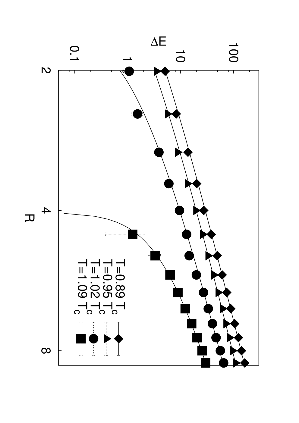
The interface energy is calculated as in eqs. (12), except that is the energy of . In figure 8 we plot vs. at different temperatures. A deviation from a simple power law at small sizes is evident. A fit of at the lowest temperature with the functional form (19) (not shown) and gives
| (20) |
Reversing the procedure (i.e. fixing and fitting in using (19)) gives . Finally, fixing both and and , still gives an excellent fit of vs. (figure 8). Since we know that cannot exceed 2, this consistency check confirms the value of found before.
V Discussion
Our result is somewhat sensible and not particularly exciting: it is basically telling us that disorder in a supercooled liquid is not strong enough to change in any exotic way the leading term of the surface energy cost: surfaces remain surfaces, albeit a bit rough. is not actually a part of AG theory, so it is more proper to compare with RFOT, where was originally introduced. It must be said that the value derived in [4] using RG arguments always had its greatest appeal in the fact that, together with , it gave back the VFT equation (11). In fact, the arguments used in [4] to fix do not belong to RFOT itself, and other values are in principle compatible with the conceptual structure of RFOT. On the contrary, the value found for within RFOT has to do with a crucial aspect of the theory. Hence, it seems that the real interesting comparison is about the exponent , after all.
The value we find implies that the barrier for the rearrangement of a correlated region scales linearly with its size,
| (21) |
The proposal of AG, , has always seemed a bit exaggerated, since one can imagine several ways for the system to pay less than the entire volume to rearrange a region. One of this ways, and not the most pedestrian, is suggested by the fact that the greatest part of the energy necessary to create the excitation is stored in the interface. Hence, one may expect that the barrier scales with the same exponent as the surface energy cost, i.e. . This is, basically, the idea of RFOT. We note that such idea is deeply rooted in the theory of nucleation, which was a indeed a source of inspiration for the original formulation of RFOT. A proportional relationship between inverse diffusion constant and the exponential of the number of particles belonging to a dynamically correlated cluster has been reported for a model of water [22], but this is not necessarily in contradiction with the above. The dynamical clusters and the excitations of RFOT (or AG’s cooperatively rearranging regions) are probably different entities, as mentioned above. Furthermore, the simulations of ref. 22 correspond to a different temperature regime (above the mode-coupling temperature) and the objects found in that work are rather noncompact, with different volume/surface ratio from the excitations we are studying.
According to RFOT there are two competing forces: the free-energy cost to create an excitation, scaling as , and the configurational entropy gain due to the change of state of the rearranging region, scaling as . In these two expressions is the surface tension and is the configurational entropy. Hence, the total free energy for the formation of the excitation is, according to RFOT,
| (22) |
At this point, RFOT, in perfect analogy with nucleation theory, proceeds by finding the maximum of such non-monotonous function (recall that ). This maximum provides two essential pieces of information: First, the position of the maximum, , gives the critical size of the rearranging region, i.e. the mosaic correlation length (cf. eq. 3),
| (23) |
Second, and most important for us now, the height of the maximum, , gives the size of the free-energy barrier to be crossed to rearrange the region,
| (24) |
This fixes , and it coincides with the intuitive notion that the barrier should scale the same as the interface cost.
This last result, however, is at variance with what we find here, relation (21): in fact, whatever one thinks about our numerical result for , a value of as small as seems rather unlikely. In any case, it is important to emphasize that is a consequence of the maximization of eq. (22), which in turn follows from the nucleation paradigm. It has been noted, however, that nucleation is perhaps not a fully correct paradigm to describe the formation of amorphous excitations within a deeply supercooled liquid [23]. The essence of RFOT, namely the competition between a surface energetic term and a bulk entropic term, retains its deepest value even if we do not cast it within the strict boundaries of nucleation theory. The value of the correlation length may come from the point where the two contributions balance, rather than from the maximum of (22), and (for obvious dimensional reasons) one gets the same expression (23) for (up to an irrelevant constant), while remains undetermined. These points are discussed in depth in [23]. Here we simply note that our present results are quite compatible with RFOT in the form it has been recast in [23], without reference to a nucleation mechanism.
Regarding the comparison between and there is a final point we have to discuss. The reader familiar with spin-glass physics will probably remember the Fisher-Huse (FH) inequality, [24],
| (25) |
which is plainly violated by the values we find here. The physical motivation of (25) is basically the following: if we represent the excitation as an asymmetric one dimensional double well, where the abscissa is the order parameter and the ordinate is the energy of the excitation, the height of the barrier (which scales as ) is always larger than (or equal to) the height of the secondary minimum (which scales as ), and hence .
How comes, then, that we find ? The FH argument was formulated in the context of the droplet picture for spin-glasses, where there are only two possible ground states. In supercooled liquids, in contrast, a rearranging region can choose among an exponentially large number of target configurations. Under this conditions, even though the FH bound still applies to the energy barrier, there may be a nontrivial entropic contribution that decreases the free energy barrier to rearrangement. We determine by measuring a time, and hence a free-energy barrier, not an energy barrier, so that the FH constraint does not necessarily hold in the case of supercooled liquids. This entropic effect is absent in the original FH argument due to the lack of exponential degeneracy of the target configurations (in fact, one would expect relation (25) to hold even in the mean-field picture of spin-glasses, where the number of ground states is large but the configurational entropy is still zero). How the FH argument should be modified in the presence of such large entropic contribution is however not clear at this point.
VI Conclusions
We have determined numerically (in ) the exponents linking the size of rearranging regions to barrier height () and to surface energy cost (). This is to our knowledge the first direct measure of these exponents. We find
| (26) |
Both values are in disagreement with those assumed by the AG and RFOT schemes. However, if we stick to eq. (8), we still obtain for the relaxation time the VFT relation (11). It seems that, albeit changing all cards on the table, we managed to get back the most used fitting relation in the physics of glass-forming systems. We stress that there is no particular reason to stick to such VFT In fact, as it has been remarked many times before, a generalised VFT with an extra fitting exponent , such that , would do an even better job in fitting the data. Yet, to get back VFT as the product of the independent numerical determination of two rather different exponents, remains a rewarding result to some extent.
Finally, let us remark that the disagreement between our exponents and those proposed in the original RFOT do not imply as harsh a blow to RFOT as it might seem at first. RFOT can be cast in a form [23] that retains its most essential aspect, namely the competition between a surface energy cost and a bulk energy gain, without using nucleation theory. If one does this, the exponents and remain unrelated and compatible with our findings. Within this context, our result seems to be an indication that RFOT is a better theory if one does not push the nucleation analogy too hard.
VII Acknowledgements
The authors thank G. Biroli, S. Franz, and I. Giardina for interesting discussions, and ETC* and CINECA for computer time. The work of TSG was supported in part by grants from ANPCyT, CONICET, and UNLP (Argentina).
Appendix A Definition of the local overlap
A suitable definition of the overlap, for the off-lattice system considered, is given using a method similar to that used in [25]: we divide the system in small cubic boxes with side and, having two configurations and , we compute the quantity
| (27) |
where is when the box with center at coordinates contains at least one particle and it is when the same box is empty. To each box we assign the weight
| (28) |
The global overlap between these two configurations and is given by
| (29) |
where runs over all boxes in the system.
We are interested in the local value of the overlap at distance from the centre of the sphere. The definition of the local overlap for a spherical corona between and is given by considering in (29) only the sum of boxes belonging to this region.
References
- [1] M. D. Ediger, Annu. Rev. Phys. Chem. 51, 99 (2000).
- [2] G. Biroli, J.-P. Bouchaud, A. Cavagna, T. S. Grigera, and P. Verrocchio, Nature Physics 4, 771 (2008), eprint arXiv:0805.4427.
- [3] S. Franz and A. Montanari, Journal of Physics A Mathematical General 40, 251 (2007), eprint arXiv:cond-mat/0606113.
- [4] T. R. Kirkpatrick, D. Thirumalai, and P. G. Wolynes, Phys. Rev. A 40, 1045 (1989).
- [5] G. Adam and J. H. Gibbs, J. Chem. Phys. 43, 139 (1965).
- [6] T. B. Schrøder, S. Sastry, J. C. Dyre, and S. C. Glotzer, J. Chem. Phys. 112, 9834 (2000).
- [7] S. C. Glotzer, J. Non-Cryst. Solids 274, 342 (2000).
- [8] B. Bernu, J. P. Hansen, Y. Hiwatari, and G. Pastore, Phys. Rev. A 36, 4891 (1987).
- [9] G. Parisi, Physical Review Letters 79, 3660 (1997).
- [10] J.-P. Hansen and I. R. McDonald, Theory of simple liquids (Academic Press, 1976).
- [11] T. S. Grigera and G. Parisi, Phys. Rev. E 63, 045102 (2001), eprint arXiv:cond-mat/0011074.
- [12] J. N. Roux, J. L. Barrat, and J.-P. Hansen, Journal of Physics Condensed Matter 1, 7171 (1989).
- [13] G. Navascues, Rep. Progr. Phys. 42, 1131 (1979), URL http://stacks.iop.org/0034-4885/42/1131.
- [14] Y. Imry and S.-k. Ma, Phys. Rev. Lett. 35, 1399 (1975).
- [15] T. Halpin-Healy and Y. Zhang, Phys. Rept. 254, 215 (1995).
- [16] C. Cammarota, A. Cavagna, G. Gradenigo, T. S. Grigera, and P. Verrocchio, ArXiv e-prints (2009), eprint 0904.1522.
- [17] D. A. Huse and C. L. Henley, Physical Review Letters 54, 2708 (1985).
- [18] T. Halpin-Healy, Physical Review Letters 62, 442 (1989).
- [19] J. Nocedal, Mathematics of Computation 35, 773 (1980).
- [20] E. T. Seppälä, M. J. Alava, and P. M. Duxbury, Phys. Rev. E 63, 066110 (2001), eprint arXiv:cond-mat/0102318.
- [21] K. P. J. Kytölä, E. T. Seppälä, and M. J. Alava, Europhysics Letters 62, 35 (2003), eprint arXiv:cond-mat/0301604.
- [22] N. Giovambattista, S. V. Buldyrev, F. W. Starr, and H. E. Stanley, Phys. Rev. Lett. 90, 085506 (2003).
- [23] J.-P. Bouchaud and G. Biroli, J. Chem. Phys. 121, 7347 (2004), eprint arXiv:cond-mat/0406317.
- [24] D. S. Fisher and D. Huse, Phys. Rev. B 38, 373 (1988).
- [25] A. Cavagna, T. S. Grigera, and P. Verrocchio, Physical Review Letters 98, 187801 (2007), eprint arXiv:cond-mat/0607817.