Atom-ion quantum gate
Abstract
We study ultracold collisions of ions with neutral atoms in traps. Recently, ultracold atom-ion systems are becoming available in experimental setups, where their quantum states can be coherently controlled. This allows for an implementation of quantum information processing combining the advantages of charged and neutral particles. The state-dependent dynamics that is a necessary ingredient for quantum computation schemes is provided in this case by the short-range interaction forces depending on hyperfine states of both particles.
In this work we develop a theoretical description of spin-state-dependent trapped atom-ion collisions in the framework of a Multichannel Quantum Defect Theory (MQDT) and formulate an effective single channel model that reduces the complexity of the problem.
Based on this description we simulate a two-qubit phase gate between a 135Ba+ ion and a 87Rb atom using a realistic combination of the singlet and triplet scattering lengths. We optimize and accelerate the gate process with the help of optimal control techniques. Our result is a gate fidelity within µs .
pacs
34.50.cx,37.90.+j,03.67.Bg,03.67.LxI introduction
Ongoing developments in quantum information processing stimulate an intense search for physical systems suitable for its implementation. Beside solid-state and photonic systems, cold ions and neutral atoms represent major candidates in this direction.
Neutral atoms can be accurately manipulated in dipole traps [1, 2], optical lattices [3] or on atom chips [4, 5] . Advanced evaporative and laser-cooling techniques allow their preparation in the vibrational ground state of different trapping potentials. Single ions can be confined in Paul or Penning traps [6] and sideband laser cooling allows to cool them down to the trap ground state.
Ultracold systems combining ions and neutral atom are currently being explored [7, 8, 9]. Besides several new quantum mechanical aspects of this system, the studies are motivated by potential applications. For example techniques of sympathetic cooling of trapped atoms by laser-cooled trapped ions can be developed [10, 11]. In this paper we propose a scheme for a quantum gate that combines the advantages of atoms and ions for quantum computation.
The trapping potentials of atoms and ions, although both built up with oscillating electromagnetic fields, do not interfere with each other, since the oscillation frequencies of the respective fields typically differ by orders of magnitude. The strength of the effective ion potential can be much stronger than for neutral atoms. Tight confinement enables fast transport and together with the good addressability of single trapped ions with lasers, this is among the advantages of ions for implementing quantum computation.
Realization of the Mott insulator phase allows to prepare an array of atoms with well controlled number of particles in a single site of an optical lattice. In comparison to ions
The possibility to prepare an array of atoms in the Mott insulator phase in an optical lattice combined with the long decoherence times of neutral atoms is a reason to use atoms for the storage of quantum information. Furthermore, the two-particle interaction of an atom and an ion is typically much stronger than for two neutral atoms, which allows fast gate operations.
While qubits can be stored in internal electronic degrees of freedom of both kinds of particles, the state dependent dynamics suitable for two-qubit gates requires engineering of the two particle interaction. To this end one can use external electromagnetic fields, e.g. magnetic Feshbach resonances that allow for a precise tuning of the two-body effective scattering properties. The long-range atom-ion interaction also supports a trap-induced type of resonance [12], because of their generally state dependent nature, they will constitute a basic element of our quantum computation scheme.
In this work we solely make use of these trap-induced shape resonances that occur at relatively large distances. In this way we avoid some possible unwanted processes that may result from molecular dynamics at short distances. We nevertheless plan to include magnetic Feshbach resonances to our theory, which can be applied to perform two-qubit operations in a controlled collisions [13, 14].
A possible setup for quantum computation is schematically depicted in Figure 1. Atoms are stored in an optical lattice in a Mott insulator phase such that each lattice site is occupied by exactly one atom. One movable ion is used to create long-distance entanglement between pairs of atoms and to perform quantum gates. The basic ingredient of this idea is the controlled and qubit-sensitive interaction between atoms and ions. In this paper we focus on the dynamics of a single atom interacting with a single ion, nevertheless; our approach can be easily extended to the situation of many atoms, or more than one ion, at a later stage.

In this work we develop a theoretical model for spin-dependent atom-ion collisions. For the case of an alkaline-earth ion and an alkali atom we formulate a model based on the Multichannel Quantum Defect Theory (MQDT) [9] taking into account the presence of trapping potentials [15]. Within our model the atom-ion interaction is described by the long-range polarization potential combined with a set of quantum-defect parameters representing the effect of the short-range potential. The essential parameters for our approach are the singlet and triplet scattering lengths, which are not yet known with sufficient accuracy, but can probably be measured in upcoming experiments. In our paper we discuss several different regimes for the values of the singlet and the triplet scattering length. For some specific range of scattering lengths we are able to reduce the complexity of the problem by employing an effective single-channel model for the atom-ion dynamics.
Using the effective single-channel description we are able to simulate a two-qubit phase gate for an arbitrary combination of atom and ion species. Applicability of the model, however, requires values of singlet and triplet scattering lengths that are nearly equal. In this case, within the single-channel description and for a specific system of 135Ba+ ion and 87Rb atom, we develop a phase gate process yielding a fidelity of within the gate time of µs. Being equivalent to the CNOT gate, the phase gate is universal for quantum computation [16]. Therefore we demonstrate the feasibility of quantum computation on the system under consideration. In a general situation, when the scattering lengths are not similar, the phase gate can be even faster; however this requires going beyond the single-channel effective description and is outside the scope of the present paper.
There are two main mechanisms that could lead to a failure of the quantum gate. One is the radiative charge transfer, which in our scheme leads to a loss of both particles in case of heteronuclear species. In contrast, for a homonuclear collision [8] the charge transfer results in a physically equivalent situation and therefore cannot be considered as a loss mechanism. Heteronuclear alkaline-earth ion – alkali atom systems have the advantage of a relatively simple electronic level structure, and for the systems studied so far; Na-Ca+ [11, 9] and Rb-Ba+ [17], the charge exchange rate remains much smaller than the elastic collisional rate, even in the presence of resonances. The second loss process results from spin changing collisions. In our scheme the qubits are encoded in hyperfine spin states, and collisions leading to final states outside of the computational basis have to be avoided. In the regime of applicability of our single-channel effective model, the coupling between different channels is by definition very weak and those kinds of losses can be safely neglected. Even in a general situation, anyway, a multichannel treatment including all possible spin-state channels offers the possibility to gain control over spin-changing processes by appropriate engineering of the gate dynamics.
The paper is organized as follows. In Sec II we describe the basic setup and model used throughout the paper. Further we briefly discuss the atom-ion polarization interaction and we introduce the concepts of correlation diagrams and trap induced resonances. The MQDT for trapped particles as well as its reduction to a single-channel model is developed in Sec III. The presented theory allows for computation of eigenstates and eigenenergies either in single-channel or multi-channel situations. The dynamics of atom-ion collisions is discussed in Sec. IV, where correlation diagrams and the Landau Zener theory help to understand the features of the system. Sec.V presents the concepts and results of our two-qubit phase gate simulations. A summary of our results, together with further perspectives and ideas, is given in Sec VI.
II Basic Setup and Model
We consider a system consisting of a single atom and a single ion, stored in their respective trapping potentials. Such potentials can be created with rapidly oscillating (rf) electric fields for ions and with optical traps based on the ac Stark effect for atoms. These traps can be well approximated as effective time-independent harmonic traps, as long as the particles are close to the ground state of the potential. For this setup we introduce an effective Hamiltonian
| (1) |
where is the mass of the ion (atom), and denote frequency and location of the harmonic trapping potential of the ion (atom) and is the interaction potential. A microscopic derivation of the Hamiltonian Eq. (1) can be found in [12]. Here, for simplicity we have assumed spherically symmetric trapping potentials and the same trapping frequencies for atom and ion: . We stress, however, that our approach can be easily generalized to anisotropic trapping potentials and different trapping frequencies [12]. A general treatment would imply coupled center-of-mass (CM) and relative degrees of freedom, thus a six dimensional equation, but there are no fundamental difficulties. In experiments both traps can be designed to be spherically symmetric, while the assumption of the same trapping frequencies allows us to decouple the relative and CM motions, thereby reducing the dimensionality of the problem from six to three. This choice simplifies our numerical calculations, on the other hand it allows to capture the most important features of the system.
We transform the Hamiltonian Eq. (1), introducing CM and relative coordinates, and , respectively. Without loosing generality we can choose the coordinate frame such that the vector of trap separation points in the direction. In this way we obtain the relative Hamiltonian
| (2) | |||
| where denotes the reduced mass of the atom-ion system and | |||
| (3) | |||
is the Hamiltonian for the special case .
II.1 Atom-ion interaction
At large distances the atom-ion interaction potential has the asymptotic behavior (). This results from the fact that the ion charge polarizes the electron cloud of the atom, and the induced dipole and the ion attract each other. Therefore, the atom-ion interaction falls into an intermediate category, between the long-range Coulomb forces and the van der Waals forces for neutral atoms. The interaction constant can be expressed in terms of the electric dipole polarizability of the atom in the electronic ground state (S-state): . The electron charge is denoted as . At short distances the interaction is dominated by the exchange forces, and higher order dispersion terms (, ) also become relevant. In our approach we model the short-range part of the potential using the quantum-defect method, that is we do not require the knowledge of the exact form of the short-range interaction. The interaction potential, in addition to the model potential, is depicted schematically in Fig. 2.

By equating the interaction potential to the kinetic energy we can define some characteristic range and corresponding characteristic energy of the atom-ion interaction. Table 1 gives the characteristic range and energy for some example atom-ion systems. For comparison it also includes the harmonic oscillator length for kHz.
| Atom-Ion System | (kHz) | ||
|---|---|---|---|
| 135Ba+ + 87Rb | 5544 | 826 | 1.111 |
| 40Ca+ + 87Rb | 3989 | 1178 | 4.142 |
| 40Ca+ + 23Na | 2081 | 1572 | 28.545 |
II.2 Single-channel quantum defect treatment
The short range interaction potential between atom and ion is typically quite complicated and in most cases it is not known theoretically with an accuracy sufficient to determine the scattering properties in the limit of ultracold energies. In order to avoid complications while using the explicit form of the short-range potentials, we resort to the quantum-defect method, which allows to include the effects of the short-range forces in an effective way. This consists in substituting the actual potential by the reference potential at all distances (see Fig. 2), and assigning an appropriate short-range phase to the wavefunction to model the effects of the short-range potential.
We illustrate this approach by solving the relative Schrödinger equation at . To this end we apply the partial wave decomposition
| (4) |
to obtain the radial Schrödinger equation
| (5) |
for the radial wavefunctions . Here, are the spherical harmonic functions describing the angular part of the 3D wavefunction, where and are the quantum numbers of the relative angular momentum and its projection on the symmetry axis , respectively. In the limit of we can neglect trapping potential, energy and centrifugal barrier in comparison to , which yields
| (6) |
with the solution
| (7) |
where is a parameter that can be interpreted as the short range phase. In our method we treat Eq. (7) as a boundary condition that we impose on the radial wave functions at short distances, while solving the relative Schrödinger equation in the general case .
In the absence of a trapping potential, and for and , the solution Eq. (7) becomes valid at all distances. By comparing the long range behavior of Eq. (7): , with the well known asymptotic form of the -wave radial wave function: , we can relate the short range phase to the scattering length
| (8) |
which is a measurable physical quantity. We note that determines the typical length-scale for the scattering length. In this chapter we have focused only on single-channel collisions, not considering internal states of the particles. The present approach is generalized in Sec. III to the realistic multichannel situation.
II.3 Correlation diagram and trap induced resonances
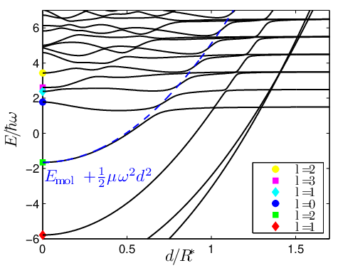
In order to obtain an intuitive understanding of atom-ion collisions, we describe them in terms of correlation diagrams, showing the energy spectrum as a function of the trap separation (see Fig. 3). Such correlation diagrams in our case connect the asymptotic vibrational states for large trap separation to the molecular and vibrational states at zero trap separation. At large distances we find harmonic oscillator-like equidistant eigenenergies that are independent of . Molecular bound states, that corresponds to the eigenstates with energies well below the zero-point vibration energy , experience a quadratic shift with the distance . This can be easily understood by noting that the bound states are well localized around , and , where is the molecular binding energy at . Beside the given arguments the quadratic shift in the molecular energy becomes immediately clear in Fig. 4. The molecular potential ‘hangs’ from the relative trapping potential in the low-distance region, thus increasing (decreasing) shifts up (down) the molecular energy as .
At some particular distances, the energies of the molecular states become equal to the energies of the vibrational levels (see Fig. 4), and the spectrum exhibits avoided crossings, known as the trap-induced shape resonances [18]. By slowly changing the trap separation we can pass through the resonance adiabatically, converting the trap vibrational states into molecular states, thus producing molecular ions. Since this process is reversible, we can coherently control the dynamics of our system by appropriately adjusting the trap distance.

III Quantum-defect theory for trapped particles
III.1 Multichannel formalism
In general, the interaction properties depend on the internal state of two colliding particles. For these internal states we choose a convenient basis, in which the two-particle Hamiltonian is diagonal at large particle distance, where the interaction potential is negligible. We then refer to the two-particle basis states as scattering channels. The wavefunction is decomposed into the chosen basis, which allows us to write down Schrödinger’s equation in matrix form. In the following we introduce an MQDT formalism, following closely the formulation by F. Mies [19], and adopting it to a situation including an external trapping potential. Assuming the same trapping frequencies for atom and ion, the CM and relative degrees of freedom are decoupled. In this case we can describe the relative motion with the close-coupled Schrödinger equation
| (9) |
Here denotes the identity matrix, is the interaction matrix, which is asymptotically diagonal
| (10) |
with indicating the channels. The trapping potential is diagonal at all distances
| (11) |
The matrix contains linearly independent solutions, where is the number of channels. The threshold energies for the molecular dissociation in channel are denoted by .
III.1.1 Special case:
For the external potential is spherically symmetric and the dynamics for different relative angular momenta is decoupled. We can decompose into a partial wave expansion
| (12) |
where Here, for simplicity we consider only the subspace. The radial wave functions fulfill
| (13) |
with
| (14) |
In our calculations we model the short-range potential by choosing appropriate short-range phases for each of the channels. This is equivalent to setting at all distances. In this case the reference potentials that are necessary to define the MQDT functions [19] can be simply taken as diagonal elements of : . Given the reference potentials, one can associate to them a pair of linearly independent solutions and of the single-channel Schrödinger equation that have WKB-like normalization at small distances
where is the local wavevector and is the WKB phase. Here, denotes a typical distance where the minima of the realistic potential occur, and the semiclassical approximation is applicable. In our modeling , and Eq. (III.1.1) describe the asymptotic behavior .
The solution to Eq. (13) can be expressed in terms of a pair of functions and :
| (17) |
Here, is the quantum-defect matrix that represents the effects of the short-range potential, in particular couplings between channels, and will be discussed later. The Matrix has constant coefficients and is determined by the boundary conditions at . We note that in MQDT the functions and describe in general only the asymptotic behavior of . Due to our choice of and , however, in our case these functions will be valid at all distances.
In analogy to MQDT in free space, we introduce another type of solutions, normalized at . At large distances the harmonic potential dominates and the solution vanishing at reads
| (18) |
where is the parabolic cylinder function, , and is the harmonic oscillator length . The two types of solutions, Eq. (III.1.1) and Eq. (18), can be related by the MQDT functions and :
| (19) | ||||
The function mixes the two solutions Eq. (III.1.1) leading to the exponentially decaying function , whereas provides the overall normalization. In fact the normalization can be calculated directly from [19]:
| (20) |
Now, the wave function can be equivalently expressed in terms of solutions normalized at infinity: ,
| (21) |
By comparing Eq. (17) with Eq. (21) one arrives at the following equation:
| (22) |
where and . This has a nontrivial solution (), if
| (23) |
which is a standard condition determining bound states in the MQDT approach. From Eq. (23) one can evaluate eigenenergies in the multichannel case, while the eigenstates are given by Eq. (21), with determined from Eq. (22). This procedure yields a set of eigenfunctions and corresponding eigenenergies , where is a constant vector, and the label enumerates the solutions:
| (24) |
Similarly to ordinary scalar wave functions, the multichannel eigenstates corresponding to different non-degenerate eigenenergies are orthonormal:
| (25) |
III.1.2 Generalization to
At nonzero trap separation, the Hamiltonian is no longer rotationally invariant, and the procedure presented in the previous section based on decoupling of states with different values of does not apply. Nevertheless, we can utilize the previous solutions at to diagonalize the full problem Eq. (9) at . To this end the total wave function is decomposed in terms of arbitrary expansion coefficients :
| (26) |
Substituting this into Eq. (9) and setting we arrive at the set of coupled equations
| (27) |
which in principle can be solved numerically with standard methods for matrix diagonalization. Here
| (28) |
and
| (29) |
III.1.3 Parametrization of and the frame transformation
In the regime of ultracold collisions, the variation of the total energy and the height of the angular momentum barrier (for the lowest partial waves which are important in the ultracold regime [9]) are much smaller than the depth of the potential at where the matrix is defined. Therefore it is justified to neglect the dependence of on both energy and angular momentum, and to set . In this way, determining the matrix at a single value of energy, we may describe the atom-ion collisions in the whole regime of ultracold temperatures.
In the paper we consider collisions of an alkali atom with an alkaline-earth ion in their electronic ground states. Hence the asymptotic channel states that are used in the Schrödinger equation Eq. (13), can be characterized by the hyperfine quantum numbers , and , for ion and atom respectively, and by the angular-momentum quantum numbers and of the relative motion of the atom and ion CM. In the rest of this section we label those channels by .
At short distances, the potential matrix becomes diagonal in the molecular basis characterized by the total electron and nuclear spins and their projections, because the short-range forces depend on the electronic configuration of the entire atom-ion molecular complex. In fact, the molecular potentials that correlate with atom and ion electronic ground states at large distances depend only on the total electron spin [9]. For our choice of species the electronic configurations are identical as in collisions of two hydrogen atoms. Thus, can take the values (singlet configuration) and (triplet configuration). Hence the quantum defect matrix , which contains the full interaction information, can be parameterized with only two constants, the singlet and triplet scattering lengths. These constants depend only on the species.
In our approach we apply a frame transformation to find in the basis of hyperfine states [20, 21]. As shown in Ref. [9], this approximation is very accurate for atom-ion collisions due to a clear separation of length scales associated with the short-range and long-range forces. On the one hand, exchange interaction becomes significant only at distances of the order of few tens of (atomic units), when the electronic wavefunctions of atom and ion begin to overlap. On the other hand, the polarization forces are very long-ranged and they are modified by the presences of the centrifugal barrier only at large distances of the order of .
III.2 Reduction to an effective single-channel model in the case of
The off-diagonal matrix elements in the quantum defect matrix are proportional to the ”coupling” scattering length, that is defined as [9]. Therefore in the case of the coupling between channels is weak and the many channel description can be effectively reduced to a single-channel model. To this end we solve the multi-channel problem at , and we find the corresponding eigenenergies and eigenstates from Eq. (22) and Eq. (23). If the mixing between channels is weak, in each of the eigenfunction , there is only one channel that dominates, i.e. the vector has only one element which is close to unity. We divide the total multichannel spectrum into distinct subsets according to the channel that gives the leading contribution to , and for each of the subset we determine the effective short-range phase (or the scattering length ). This is done by matching the multichannel spectrum in each of the subsets with the single-channel generated by Eq. (5) with the quantum-defect parameter . In the limit of zero coupling between channels, the effective scattering length is equal to . In the presence of weak coupling, is in general different from and , since the asymptotic channels typically correlate both to singlet and triplet molecular states at small distances. This procedure yields a set of short range phases , which are used at a later stage in the single-channel calculations. We note that the effective phases depend on the relative angular momentum, and in principle they weakly depend on the energy. We have verified, however, that within the considered range of energies limited to the bound states close to the dissociation threshold, and to a few tens of the lowest vibrational states, the variations of with the energy are negligible.
For collisions when only a single open channel exists, the remaining closed channels are typically only weakly coupled to the open channel (apart from the case of resonances), and the resulting multichannel wave function is dominated by the open-channel component. The situation changes, however, when there are more open channels, and the channel mixing can be significant. We have investigated this issue numerically, picking the specific ion and atom pair 135Ba+–87Rb and the trapping frequency kHz. We have considered collisions within the subspace, assuming that initially the particles are prepared in the channel . This choice is relevant for our modeling of the quantum gate, as we show later. For the collision energies above the dissociation threshold of the channel , a second open channel exists, with . In this case we find that admixture of the two remaining closed channels is negligible, whereas the contribution of both channels and in the multichannel eigenstates is typically large, and the contributions from and cannot be separated. The only exception is the case of similar and , where the inter-channel coupling is small, and the multichannel eigenstates are dominated by the single-channel contributions.
We estimate the validity of the single channel approximation by calculating the overlap of the exact multichannel and the single channel wave functions, in the range of trap separations , interesting for our dynamics. The minimum over yields some overall fidelity related to the reduction to the single channel model. For similar singlet and triplet phases, we have , and the multichannel wave functions differ from their single-channel counterparts by the presence of negligible contributions in the channels others than the dominating one. The relative contributions of individual channels are given by the vectors that are obtained in the calculation of eigenstates at . When one has to take into account that the multichannel wave functions are linear combinations of the solutions at (see Eq. (26)), and the overlap between single- and multi-channel eigenstates is a linear combination of the overlaps calculated at with the expansion coefficients given by .
Resonances occurring at can lead to significant channel mixing for few states, although the average fidelity is very high. The more these highly mixed states contribute to the wavefunctions, the larger is the error of the model. For the error estimation used in this work, we only use the trap ground state at maximal and a molecular state at minimal of interest. We find that the two fidelities lie in the same range, thus we take the minimum of them and assume the result as a lower bound for the fidelity at intermediate distances. We have additionally verified that reductions to the single channel model works best for positive values of singlet and triplet scattering lengths around .
IV Atom-ion dynamics
Traps for individual ultracold atomic particles used in schemes for quantum information processing provide in most cases for the ability to manipulate the particles’ motion via appropriate tuning of external trap parameters. This is in particular the case for optical lattices and Paul traps, where field polarizations and intensities can be changed to control the shape and position of the traps to a high degree of accuracy. Our proposal relies on these standard techniques, thereby introducing the innovative aspect of combining traps for ions and atoms. As already discussed elsewhere [12], the physical mechanisms generating the traps for ions and atoms are different and lead, under appropriate conditions, to independent microscopic traps, which can be modeled as follows.
In this chapter dynamics will be described by introducing a time dependent trap displacement . Below a certain distance , the eigenenergies of the system start to depend on the spin state as well as on itself, and positions of trap-induced resonances are determined by the internal state of both particles. In this way trap displacement can be used for spin-dependent control of the atom-ion system.
IV.1 Landau-Zener Theory
The Landau-Zener formula gives a basic understanding of the atom-ion dynamics in the vicinity of trap-induced shape resonances. It describes a general two-level system whose eigenstates and are coupled by some kind of interaction, and in which the two eigenlevels and form an avoided crossing when varying an external parameter. In our case this external parameter is the trap displacement . The probability of a nonadiabatic passage of the crossing [12],
| (30) |
depends on the coupling matrix element, the velocity of passage of the resonance and the relative slope of the levels, where . A fast passage of the avoided crossing () results in a nonadiabatic evolution, preserving the shape of the wave function. At small velocities the resonance is passed adiabatically (), i.e. the system follows its eigenenergy curves. In the trapped atom-ion system, for certain trap separations, the energy of some molecular bound states becomes equal to harmonic-oscillator energies, resulting in the avoided crossings. If such avoided crossing is passed adiabatically, then the initial harmonic-oscillator state with atom and ion located in their separated traps can evolve into a molecular bound state, where the atom and ion are trapped in a combination of the two external potentials. This process is reversible and we use it in Sec. V to realize an entangling two-qubit operation.
In order to precisely predict the outcome of a collision process, in our simulations we have calculated time evolution numerically, using the Landau-Zener formula only as a guide to estimate the relevance of the avoided crossings for the transfer process. Since the energy of the molecular bound states changes according to (see Fig. 3), deeply bound states can cross vibrational states only at large . In this case avoided crossings are very weak, due to the fact that decays exponentially with the trap distance [12]. Hence, the deeply bound states have no relevance for the dynamics and in our simulations we have included only shallow bound states that are closest to the dissociation threshold.
IV.2 Full dynamics in the single-channel model
In the case of similar and , when the effective single-channel description is applicable, we describe the dynamics of the controlled atom-ion collision with the following time-dependent Hamiltonian:
| (31) |
We decompose the corresponding time-dependent wavefunction in the basis of the eigenstates at
| (32) |
in analogy to Eq. (26). Substituting this into Schrödinger equation, we obtain a set of coupled differential equation for the expansion coefficients :
| (33) |
Here, is the dipole matrix element, which in the context of the multichannel formalism is defined in Eq. (28). We determine the radial part of the single channel wavefunctions and the eigenenergies with the Numerov method [22], using the effective short range phase as a boundary condition at minimal distance. From the wavefunctions, one can calculate the matrix elements . Inserting these into Eq. (33), we are able to solve the equation for the coefficients numerically with standard routines. Thereby we verify in each case that our basis, limited by the maximal values of the and quantum numbers, is large enough and that the results do not change when increasing the basis.
By comparing exact numerical dynamics with the results predicted by the Landau-Zener theory, we have found, for example, an error of about 0.5% for the probability of a fast, diabatic passage of the avoided crossing at in the spectrum of Fig. 6a, with a speed of 1 mm/s. Similar good agreement was observed in the adiabatic limit, and only for intermediate speeds we found discrepancies of the order of 10%. This might be due to the complexity of the spectrum, which makes it impossible to isolate an avoided crossing between two eigenstates from the influence of the rest of the eigenstates. Thus, the Landau-Zener theory is not applicable for quantum gate calculations performed for example in Sec. V.5.1. Also, faster processes lead to excitations to higher vibrational states that cannot be described by the Landau-Zener theory.
V Quantum gate
V.1 Qubit states
In this Section we apply our model of the spin-state-dependent atom-ion collisions to construct a two-qubit controlled-phase gate. We encode qubit states in hyperfine states of atom and ion. According to our previous notation, a given two-particle spin state is referred to as a channel . The total spin projection is a conserved quantity during the collision. Therefore two states of unlike cannot be coupled. In our case it is convenient to pick the computational basis states
| (34) |
according to Fig. 5, leading to the two-qubit states
| (35) |
Each of the two-qubit states is represented by a scattering channel. The state has and is coupled to seven other channels, which have higher dissociation energies and therefore they remain closed for collisions. Thus the state is stable with respect to spin-changing collisions. The channels and , belonging to the subspace, are coupled to each other and to two other channels, that are closed for both and collisions. There is no coupling for the state , since it is the only state in the subspace. In this way our choice of the qubit states minimizes the possibility of spin-changing collisions, and the only process that can lead to potential losses is the inelastic collision .

V.2 Dynamics of four isolated channels
Our multichannel theory describes collisions between atom and ion for general spin states of particles, in particular for the four qubit states introduced in Eq. (35). For simplicity of the numerical calculations, here we do not perform the full multichannel dynamics, but rather we focus on the regime of applicability of the effective single-channel model, described in Sec. III.2. For every choice of parameters assumed in our calculations, we verify that the coupling to other spin states can be neglected. The total Hamiltonian including external degrees of freedom, for the subspace corresponding to our computational basis, reads
| (36) |
We denote a qubit channel by with . Linear combinations of the computational basis states form a general two-particle state , where denotes the quantum state of the atom-ion relative motion for the channel . Obviously, the time evolution of
| (37) |
is determined by the dynamics of the spatial part of the wave function , which we evaluate from Eq. (33). On the other hand, the phases due to the differences in threshold energies in each of the channels, do not lead to state dependent dynamics, and can be eliminated by single qubit operations (see discussion in the next subsection).
V.3 Phase gate process
The two-qubit phase gate is represented by the transformation
| (38) |
performed on the computational basis states. The first step is the controlled interaction of atom an ion that leads to a specific phase for each two-qubit state. By applying the single-qubit transformation we can undo three of these phases and assign the total gate phase
| (39) |
to the state [23]. If this phase equals , the phase gate, combined with single qubit gates, is a universal gate for quantum computation, as it is equivalent to a CNOT gate. It is possible to realize this phase gate scheme within our single-channel model, since the transformation of each two-qubit basis state can be treated separately.
For our gate scheme, atom and ion are initially prepared in the motional ground state of their respective traps. The channel phases are gained by the control of the relative motion of atom and ion during the collision. Ideally we aim at obtaining back the motional ground state at the end of the gate process, so that the phase accumulated by relative motion is assigned to the qubit state.
V.4 Gate fidelity
Our definition of the fidelity is based on the overlap of the initial state of relative motion with the final state . In an ideal process these states are equal up to a state dependent phase. The fidelity needs to account for this phase. For one channel and at zero temperature, according to [24] we can define the fidelity as follows
| (40) |
where is the difference between the desired channel phase and the phase obtained by actual time evolution. In the following, we will assume that according to Eq. (38) the phases for the channels , and are undone perfectly due to the single qubit rotations leading to , while is nonzero. Hence, for channels , and the fidelity is restricted only by the overlap between initial and final states, while for the state we additionally require that the total gate phase, computed from the single-channel phases with Equation (39), is .
We can further define the overall gate fidelity as
| (41) |
since in our model the channels are decoupled (we neglect spin changing collisions).
V.5 Adiabatic regime
The adiabatic dynamics can be understood with the help of the correlation diagrams introduced in Sec. II.3. Our gate scheme aims at an adiabatic transfer from an initial oscillator state to a molecular state , and back to the initial state. This is achieved by a variation of the trap distance across an appropriate avoided crossing, which we choose after investigating the correlation diagram. For example, the resonance at the trap distance in Fig. 6a appears strong enough and we use it in numerical calculations in the following. During the transfer process each logical basis state acquires a different phase, since the energies of molecular states depend on the channel (see Fig. 6b). The phase accumulated for each channel in an adiabatic transfer process is given by the integral
| (42) |
where is the energy of the adiabatic eigenstate depicted as a function of in Fig. 6 (thick curve). In the adiabatic regime we avoid excitations to higher vibrational states by keeping the velocity small, compared with the characteristic velocity of the harmonic motion in the trap: . On the other hand we choose the velocity across weaker resonances at larger distances high enough to pass them diabatically, as seen in Fig. 6. We want to find a particular function , which, if applied on the trapped atom-ion system, results in a desired total gate phase, while ensuring diabatic passage of the weak resonances as well as adiabatic passage of the strong resonance. Since the total phase depends on the difference between single-channel phases (see Eq. (39)), the gate speed, in fact, is determined by the differences in the potential energy curves of unlike channels.
For the sake of concreteness we assume specific values of the singlet and triplet scattering lengths, in such a way that our single-channel effective model is applicable. For our calculations we choose and . According to the procedure described in Sec. III.2 the estimate of the error introduced by the model is . For singlet and triplet scattering lengths that differ by more than the channel mixing becomes already significant and does not allow for a single-channel description.
Actually, the singlet and triplet scattering lengths are uniquely determined by the specific choice of the atom-ion system we describe. So far these parameters have not been measured experimentally, for any atom-ion system. However, as soon as the accurate values of and are determined, one can repeat the calculations with the physically correct parameters, which may require going beyond the single-channel model, and including the full multichannel dynamics according to Sec. III.
Assuming the single-channel effective model we first compute a correlation diagram for each of the channels. This is done by diagonalizing the Hamiltonian in the basis of eigenstates evaluated at . The result is depicted in Fig. 6a for the channel. The diagrams show small differences in the molecular states at small distances (Fig. 6b), since the energy of molecular states depends on the atom-ion spin configuration (the qubits).


V.5.1 Numerical simulation of an adiabatic phase gate
In our simulation of the gate process the initial and final trap separations coincide: . We assume that initially the atom and ion are each in the ground-state of its own trap. The distance is determined in such a way that there are no bound states in the vicinity of that would influence the harmonic-oscillator ground-state.
The controlled time evolution of our atom-ion system requires the appropriate adjustment of the distance between the two trapping potentials as a function of time. The slope of this function is essential for the result.
In order to follow the energy curve depicted in Fig. 6a, we construct a specific function . We start at with an initial velocity , which is large enough to traverse weaker resonances diabatically. On the other hand, much larger velocities would cause unwanted motional excitations in the trap. At , the velocity is decreased to in order to adiabatically convert the trap state into a molecular bound state using a stronger resonance. The curve is followed down to some minimal distance . Then, the reversed pulse brings the system to the initial trap separation. Fig. 7a shows the complete function. It is known that sharp kinks can cause motional excitations, therefore we use a smooth function to change between two slopes and . Here, the sign is used for increasing(decreasing) slope, is an offset and is a parameter adjusting the curvature at the kink. Around the turning point at .
We can now compute the solution of the Schrödinger equation numerically at a given time by solving Eq. (33) with standard numerical routines . This yields the gate phase which, for example, can be adjusted by a variation of . This phase is in fact a phase difference accumulated due to the energy splitting
| (43) |
shown in Fig. 8 as a function of trap separation; the larger , the faster a phase difference is reached. Thus, decreasing increases the phase, as seen in Fig. 7b. We find a gate phase of at . The corresponding gate fidelity is according to Eq. (41). The process takes the time , which equals ms for our choice of the trapping frequency kHz and the masses and hyperfine structure of the 87Rb atom and the 135Ba+ ion. We show the population of the instantaneous eigenstates in Fig. 9. At the trap ground state is labeled with . The system is initialized in this state. At half gate time the quantum state changed to , which is the molecular state at . Finally, at the end of the gate process, we almost perfectly obtain back the initial state.


V.6 Fast gate using optimal control
Quantum optimal control techniques are a powerful tool that allows to increase the fidelity of a time evolution process by finding an appropriate pulse shape for some external control parameter. The outcome of the controlled collision of an atom and an ion is very sensitive to the particular shape of the time dependence in the trap distance . It is hard to manually design a specific function that leads to a phase gate fidelity very close to unity.
The most significant problem in our specific example calculation results from a relatively weak resonance at , which we want to pass in a non-adiabatic way. We could not find an optimal constant slope that brings us from the trap state at to the trap state with across the resonance without losses. Large velocities lead to excitations of energetically higher states, while the consequence of smaller velocities is a non-negligible population of the molecular state that crosses the trap state. This population is not fully recovered on the way back. In Sec. V.5.1 we nevertheless found a process that yields a gate fidelity of .
With optimal control we can not only find a pulse shape that produces a satisfactory gate fidelity, but also go beyond the adiabatic regime and reduce the gate time. By applying larger velocities, we allow for excitations to higher energy levels. Making use of interference effects, an appropriate pulse shape can undo these excitations in the final state of the process.
This optimal pulse shape is found here with an iterative optimization algorithm called intermediate feedback control, which is for example introduced in [13]. We start with an initial guess for the control function , which in general does not yield a satisfactory fidelity. The fidelity of the process is increased in every iteration step by updating . We divide the time axis in small time steps . At each time step we evolve the wave function forward in time using the Crank-Nicholson scheme [25]. The update of is successively performed in every time step.
V.6.1 Enhancing the fidelity of the adiabatic gate
The adiabatic gate process of Sec. V.5.1 has the fidelity . With only three iterations of the optimal control algorithm we can enhance this fidelity to , which even exceeds the validity of the underlying single-channel model. The gate phase is improved to . The optimized function shows small scale variations (’wiggles’) that are a typical feature of the used optimization algorithm. These wiggles have the amplitude nm and happen on a time scale of the order of µs. This amplitude is smaller than the uncertainty of the ion trap center position in up-to-date experimental realizations.
V.6.2 Fast Gate Scheme
It is desirable to reduce the gate time to a minimum. In our case this minimum is given by the time that is at least required for accumulating the gate phase . We profit from the energy differences of the molecular states for the different channels. The differences are largest at small distance , but below they are practically constant. The fastest possible gate needs to effectively transport the atom-ion relative wavefunction into a molecular state, where the gate phase is accumulated during a certain time. The gate ends with a reversed pulse and brings the system to the initial trap ground state, while the logical phase is preserved.
The optimal control algorithm can be used to build such a gate process. As a first step we design changing the quantum state of atom and ion from the trap ground state at to the molecular state at , for all channels during the transport time . The optimization objective for this step aims at maximizing the overlap of the time-evolved state with the desired molecular state. The second step is a stationary evolution at , where the main part of the differential phase is accumulated. Subsequently we perform the reverse of the initial pulse. The combined pulse is shown in Fig. 10a.
The total gate time is µs. With respect to the adiabatic case this means a reduction by a factor of 4.Since our scheme makes use of the channel energy differences in the molecular state at , we can estimate a quantum speed limit for this process , with from Eq. (43), which gives the minimal gate time, neglecting transport durations and infidelities of the molecular state’s population. In our example this limit is µs. Our gate process time lies very close to this value, considering an overall transport time of µs. We note that a part of the phase is accumulated during the transport phase, since we already enter the regime where the energy differences become significant.
Further reducing the transport time may be possible, but the optimization algorithm we used stopped converging in reasonable time for larger transport velocities. However, we already could significantly accelerate the process utilizing optimal control techniques.
V.6.3 Perspectives for further improvement
Certainly the gate speed would improve if the difference between singlet and triplet scattering lengths was larger than assumed in our example calculation. In general case one can use our multichannel formalism for an accurate description of the dynamics, beyond the single-channel approximation. We point out that the essential parameters and are still unknown and they need to be measured in experiments in order to do realistic calculations for specific systems. However, our work demonstrates the feasibility of an ion-atom quantum gate even based on the simplified scheme we assume for calculations.
Further possibilities occur for very different values and . In this case especially the and states are coupled strongly. In this case optimal control mechanisms can be used to suppress effects of spin-changing collisions in the final state, in order to realize a phase gate. The coupling of and could also be effectively used for a SWAP gate, which inverts the populations of these two channels—or for its square root, which in combination with single-qubit rotations constitutes an alternative universal set of gates for quantum computation.


VI Conclusions and outlook
In this work we analyzed the spin-state-dependent interaction between a single atom and a single ion guided by external trapping potentials. We applied our insight on this system in order to realize a two-qubit quantum gate process and thereby provide the basic ingredients for quantum computation with atoms and ions combined in one setup. This work was motivated by recent experimental possibilities combining magneto-optical traps or optical lattices for atoms, and RF traps for ions. These experiments are currently established in several groups worldwide [17, 8].
We started our description of controlled interaction of an atom and an ion by formulating a multichannel quantum-defect theory for trapped particles, analogous to the free-space case discussed in [9]. This step simplifies the description of atom-ion collisions as it does not require a detailed knowledge of the molecular potentials at short range. Experiments measuring the positions of Feshbach resonances can determine the essential two parameters for our theory—the singlet and triplet scattering lengths. Since these experiments have not yet been performed, here, we have focused on the case of similar singlet and triplet scattering lengths given in order of magnitude by , while the general case of different scattering lengths have been discussed only qualitatively.
We were able to reduce the multichannel formalism to an effective single-channel model that singles out a specific spin state of atom and ion. This model is found to be accurate for similar values of the singlet and triplet scattering lengths. In calculations we have assumed and for the singlet and triplet scattering lengths, respectively. In contrast, opposite signs of scattering lengths exclude a single-channel description. We estimated the error introduced by our specific single-channel model to , which is due to a mixing of channels in the eigenstates of the system. Taking even closer values of singlet and triplet scattering lengths lead to a better applicability of the single-channel description.
Where applicable, our effective single-channel model can be implemented in calculations in the context of ultracold chemistry as well as ultracold scattering physics. A single-channel description assigning quantum-defect parameters to each channel separately was already discussed in [12]. However, the spin state was not included in previous research. In the present approach, starting from the fundamental parameters and of the multichannel formalism, we derive the quantum-defect parameters of each isolated channel consistently. We take the channel coupling into account and we estimate the error introduced by assuming isolated channels. Therefore, we can apply the model to quantum computation schemes that store qubits in internal spin states of atom and ion.
A remarkable feature of the system is trap-induced shape resonances that couple molecular bound states to unbound trap states. Quasistatic eigenenergy curves show these resonances as avoided crossings. They can be used to form ultracold trapped molecular complexes and thereby allow full control of cold chemical reactions.
Trap-induced resonances form a basis for our idea of the phase gate process as well. Initially an atom and an ion are prepared in the trap vibrational ground state. We realize a qubit-dependent two-particle phase via controlling the external degrees of freedom. By bringing the traps close together we let the particles interact and finally separate them, obtaining the motional ground state again. In doing so we cross weaker resonances diabatically (remaining in a trap state) and then follow a stronger resonance adiabatically into a molecular bound state, where a two-qubit phase is accumulated. Since the positions of the resonances are different for each spin combination, the accumulated phase is different for each qubit channel and we are able to control the trap distance in such a way that a two-qubit phase gate is realized. This phase gate, in combination with single qubit rotations, is a universal gate for quantum computation.
We performed numerical simulations of the controlled collision specifically for a 135Ba+ ion interacting with a 87Rb atom, each guided by a spherically symmetric harmonic trap with kHz. We have chosen specific hyperfine-qubit states to obtain the four qubit-channels . In this framework we developed a two-qubit phase gate process entangling atom and ion. We thereby showed that trap-induced resonances can be used to control the interaction of atom and ion. The error for our gate process is and in this case the gate time is ms. Using optimal control techniques we were able to accelerate the process to µs. In future work we plan to decrease the gate time by using higher trapping frequencies allowing faster transport.
Our choice of very similar scattering lengths allowed to perform single-channel calculations, but on the other hand it limits the gate time, as the energy splitting between the channels is rather small. A more general description can be done in the framework of our multichannel formalism, allowing for arbitrary combinations of singlet and triplet scattering lengths. It is possible that the actual values of the scattering lengths are in fact very different, which would require a more complicated multichannel computation, but also possibly allows much faster quantum gates. However, already in the regime we considered, a gate time below a millisecond is demonstrated.
In our model, we assumed harmonic trapping potentials, and the oscillator frequencies were equal for atom and ion. Among the advantages of ions for quantum computation is the existence of much tighter trapping potentials than for atoms. The basic ideas developed in this paper are expected to be applicable to such more general situations with different trapping frequencies. A generalization is highly desirable, but will lead to a more complicated theoretical treatment, as for example center-of-mass motion becomes coupled to the relative motion. Very elongated cigar-shaped traps have already been treated in previous works. One of our goals is the consideration of particular experimental realizations in order to describe them with our theory, compare the results or suggest directions of experimental research.
In the present work we did not use external magnetic fields in order to manipulate the interaction. Magnetic induced Feshbach resonances have been applied very successfully to engineer neutral atom collisions. Future investigations will include magnetic fields to control the atom-ion interaction even more efficiently and possibly combine trap-induced resonances and Feshbach resonances for this purpose. Our work can be seen as a principle investigation of a new, interesting physical system and can be extended in many directions.
Acknowledgements.
We acknowledge support by the EU under the Integrated Project SCALA, the German Science Foundation through SFB TRR21 Co.Co.Mat, the National Science Foundation through a grant for the Institute for Theoretical Atomic, Molecular and Optical Physics at Harvard University and Smithsonian Astrophysical Observatory, and the Polish Government Research Grant for the years 2007-2010. The authors would like to thank P. Zoller, P. Julienne, J. Hecker Denschlag and P. Schmidt for fruitful discussions. HDB thanks M. Trippenbach and the University of Warsaw for very rewarding two-week visit.References
- [1] S. Bergamini, B. Darquié, M. Jones, L. Jacubowiez, A. Browaeys, and P. Grangier, J. Opt. Soc. Am. B 21, 1889 (2004), URL http://www.opticsinfobase.org/abstract.cfm?URI=josab-21-11-18%89.
- [2] Y. Miroshnychenko, W. Alt, I. Dotsenko, L. Förster, M. Khudaverdyan, D. Meschede, D. Schrader, and A. Rauschenbeutel, Nature 442, 151 (2006), URL http://dx.doi.org/10.1038/442151a.
- [3] M. Greiner, O. Mandel, T. Esslinger, T. Hänsch, and I. Bloch, Nature 415, 39 (2002), URL http://dx.doi.org/10.1038/415039a.
- [4] C.-S. Chuu, T. Strassel, B. Zhao, M. Koch, Y.-A. Chen, S. Chen, Z.-S. Yuan, J. Schmiedmayer, and J.-W. Pan, Phys. Rev. Lett. 101, 120501 (pages 4) (2008), URL http://dx.doi.org/10.1103/PhysRevLett.101.120501.
- [5] R. Dumke, M. Volk, T. Müther, F. B. J. Buchkremer, G. Birkl, and W. Ertmer, Phys. Rev. Lett. 89, 097903 (2002), URL http://prola.aps.org/abstract/PRL/v89/i9/e097903.
- [6] D. Leibfried, R. Blatt, C. Monroe, and D. Wineland, Rev. Mod. Phys. 75, 281 (2003), URL http://link.aps.org/doi/10.1103/RevModPhys.75.281.
- [7] W. W. Smith and J. Makarov, Oleg P.and Lin, J. Mod. Opt. 52, 2253 (2008), URL http://dx.doi.org/10.1080/09500340500275850.
- [8] A. T. Grier, M. Cetina, F. Oručević, and V. Vuletić, Phys. Rev. Lett. 102, 223201 (pages 4) (2009), URL http://link.aps.org/abstract/PRL/v102/e223201.
- [9] Z. Idziaszek, T. Calarco, P. S. Julienne, and A. Simoni, Phys. Rev. A 79, 010702 (2009a), URL http://link.aps.org/doi/10.1103/PhysRevA.79.010702.
- [10] Z. Idziaszek, T. Calarco, and P. Zoller, (unpublished) (2009b).
- [11] O. P. Makarov, R. Côté, H. Michels, and W. W. Smith, Phys. Rev. A 67, 042705 (2003), URL http://dx.doi.org/10.1103/PhysRevA.67.042705.
- [12] Z. Idziaszek, T. Calarco, and P. Zoller, Phys. Rev. A 76, 033409 (pages 16) (2007), URL http://link.aps.org/abstract/PRA/v76/e033409.
- [13] T. Calarco, U. Dorner, P. S. Julienne, C. J. Williams, and P. Zoller, Phys. Rev. A 70, 012306 (2004), URL http://link.aps.org/doi/10.1103/PhysRevA.70.012306.
- [14] M. Krych and Z. Idziaszek, Physical Review A (Atomic, Molecular, and Optical Physics) 80, 022710 (pages 11) (2009), URL http://link.aps.org/abstract/PRA/v80/e022710.
- [15] Y. Chen and B. Gao, Phys. Rev. A 75, 053601 (pages 9) (2007), URL http://link.aps.org/abstract/PRA/v75/e053601.
- [16] A. Barenco, D. Deutsch, A. Ekert, and R. Jozsa, Phys. Rev. Lett. 74, 4083 (1995), URL http://prola.aps.org/abstract/PRL/v74/i20/p4083_1.
- [17] S. Schmid, A. Härter, J. Hecker Denschlag, and A. Frisch, private communication (2009).
- [18] R. Stock, I. H. Deutsch, and E. L. Bolda, Phys. Rev. Lett. 91, 183201 (2003), URL http://link.aps.org/doi/10.1103/PhysRevLett.91.183201.
- [19] F. H. Mies, J. Chem. Phys. 80 (1984), URL http://link.aip.org/link/?JCPSA6/80/2514/1.
- [20] B. Gao, E. Tiesinga, C. Williams, and P. Julienne, Phys. Rev. A 72, 042719 (2005), URL http://link.aps.org/doi/10.1103/PhysRevA.72.042719.
- [21] J. P. Burke, C. H. Greene, and J. L. Bohn, Phys. Rev. Lett. 81, 3355 (1998).
- [22] B. R. Johnson, J. Chem. Phys. 67, 4086 (1977), URL http://link.aip.org/link/?JCP/67/4086/1.
- [23] T. Calarco, J. I. Cirac, and P. Zoller, Phys. Rev. A 63, 062304 (2001), URL http://link.aps.org/doi/10.1103/PhysRevA.63.062304.
- [24] T. Calarco, E. A. Hinds, D. Jaksch, J. Schmiedmayer, J. I. Cirac, and P. Zoller, Phys. Rev. A 61, 022304 (2000), URL http://link.aps.org/doi/10.1103/PhysRevA.61.022304.
- [25] W. Press, S. Teukolsky, W. Vetterling, and B. Flannery, Numerical Recipes in C (Cambridge University Press, Cambridge, UK, 1992), 2nd ed.