The “$\mu$ from $\nu$” Supersymmetric Standard Model ($\mu\nu$SSM) was proposed in the literature [1, 2, 3] as an alternative to the Minimal Supersymmetric Standard Model (MSSM). In particular, it provides a solution to the $\mu$-problem [4] of the MSSM and explains the origin of neutrino masses by simply using right-handed neutrino superfields.

The superpotential of the $\mu\nu$SSM contains, in addition to the usual Yukawas for quarks and charged leptons, Yukawas for neutrinos $\hat{H}_{u}\,\hat{L}\,\hat{\nu}^{c}$, terms of the type $\hat{\nu}^{c}\hat{H}_{d}\hat{H}_{u}$ producing an effective $\mu$ term through right-handed sneutrino vacuum expectation values (VEVs), and also terms of the type $\hat{\nu}^{c}\hat{\nu}^{c}\hat{\nu}^{c}$ avoiding the existence of a Goldstone boson and contributing to generate effective Majorana masses for neutrinos at the electroweak scale. Actually, the explicit breaking of R-parity in this model by the above terms produces the mixing of neutralinos with left- and right-handed neutrinos, and as a consequence a generalized matrix of the seesaw type that gives rise at tree level to three light eigenvalues corresponding to neutrino masses [1].

The breaking of R-parity can easily be understood if we realize that in the limit where Yukawas for neutrinos are vanishing, the $\hat{\nu}^{c}$ are just ordinary singlet superfields, without any connection with neutrinos, and this model would coincide (although with three instead of one singlet) with the Next-to-Minimal Supersymmetric Standard Model (NMSSM) where R-parity is conserved. Once we switch on the neutrino Yukawa couplings, the fields $\hat{\nu}^{c}$ become right-handed neutrino superfields, and, as a consequence, R-parity is broken. Indeed this breaking is small because, as mentioned above, we have an electroweak-scale seesaw, implying neutrino Yukawa couplings no larger than $10^{-6}$ (like the electron Yukawa).

The latter also implies that processes violating lepton number that might wash-out any baryon asymmetry present in the model would be suppressed. Notice also that electroweak baryogenesis could work in this model in a similar way to the case of the NMSSM [5]. Actually, the fact that in the $\mu\nu$SSM there are three singlets instead of one like in the NMSSM, should in principle give more freedom to be able to obtain more easily electroweak baryogenesis. The detail conditions for baryogenesis in this model are presently under study [6].

Since R-parity is broken in the $\mu\nu$SSM, one could worry about fast proton decay through the usual baryon and lepton number violating operators of the MSSM. Nevertheless, the choice of $R$-parity is ad hoc. There are other discrete symmetries, like e.g. baryon triality which only forbids the baryon violating operators [7]. Obviously, for all these symmetries R-parity is violated. Besides, in string constructions the matter superfields can be located in different sectors of the compact space or have different extra $U(1)$ charges, in such a way that some operators violating $R$-parity can be forbidden [8], but others can be allowed.

Several recent papers have studied different aspects of the $\mu\nu$SSM. In [2], the parameter space of the model was analyzed in detail, studying the viable regions which avoid false minima and tachyons, as well as fulfill the Landau pole constraint. The structure of the mass matrices, and the associated particle spectrum was also computed, paying special attention to the mass of the lightest Higgs. In [9], neutrino masses and mixing angles were discussed, as well as the decays of the lightest neutralino to two body ($W$-lepton) final states. The correlations of the decay branching ratios with the neutrino mixing angles were studied as another possible test of the $\mu\nu$SSM at the LHC. The phenomenology of the $\mu\nu$SSM was also studied in [10], particularized for one and two generations of right-handed sneutrinos, and taking into account all possible final states when studying the decays of the lightest neutralino. Possible signatures that might allow to distinguish this model from other R-parity breaking models were discussed qualitatively in these two works [9, 10]. In [11], the analysis of the vacua of the $\mu\nu$SSM carried out in [2] was completed, obtaining that spontaneous CP violation through complex Higgs and sneutrino VEVs is possible. Neutrino physics and the associated electroweak seesaw mechanism was also studied. It was shown how the experimental results can easily be reproduced and explained why the mixing patterns are so different in the quark and lepton sectors. All the results were discussed in the general case with phases.

On the other hand, when $R$-parity is broken, the lightest supersymmetric particle (LSP) is no longer stable. Thus neutralinos [12] or sneutrinos [13], with very short lifetimes, are no longer candidates for the dark matter of the Universe. Nevertheless, if the gravitino is the LSP its decay is suppressed both by the gravitational interaction and by the small R-parity violating coupling, and as a consequence its lifetime can be much longer than the age of the Universe [14]. Thus the gravitino can be in principle a dark matter candidate in R-parity breaking models. This possibility and its phenomenological consequences were studied mainly in the context of bilinear or trilinear R-parity violation scenarios in [14, 15, 16, 17, 18, 19, 20, 21, 22]. In [16, 18, 19, 21] the prospects for detecting gamma rays from decaying gravitinos in satellite experiments were also analyzed. In this work we want to discuss these issues, gravitino dark matter and its possible detection in the FERMI satellite [23], in the context of the $\mu\nu$SSM.

The superpotential of the $\mu\nu$SSM introduced in [1] is given by

where we take $\hat{H}_{d}^{T}=(\hat{H}_{d}^{0},\hat{H}_{d}^{-})$, $\hat{H}_{u}^{T}=(\hat{H}_{u}^{+},\hat{H}_{u}^{0})$, $\hat{Q}_{i}^{T}=(\hat{u}_{i},\hat{d}_{i})$, $\hat{L}_{i}^{T}=(\hat{\nu}_{i},\hat{e}_{i})$, $i,j,k=1,2,3$ are family indices, $a,b=1,2$ are $SU(2)_{L}$ indices with $\epsilon_{12}=1$, and $Y$, $\lambda$, $\kappa$ are dimensionless matrices, a vector, and a totally symmetric tensor, respectively.

Working in the framework of supergravity, the Lagrangian $\mathcal{L}_{\text{soft}}$ is given by:

In addition to terms from $\mathcal{L}_{\text{soft}}$, the tree-level scalar potential receives the $D$ and $F$ term contributions also computed in [1]. In the following we will assume for simplicity that all parameters in the potential are real. Once the electroweak symmetry is spontaneously broken, the neutral scalars develop in general the following VEVs:

For our computation below we are interested in the neutral fermion mass matrix. As explained in [1, 2], neutralinos mix with the neutrinos and therefore in a basis where ${\chi^{0}}^{T}=(\tilde{B^{0}},\tilde{W^{0}},\tilde{H_{d}},\tilde{H_{u}},\nu_{R_{i}},\nu_{L_{i}})$, one obtains the following neutral fermion mass terms in the Lagrangian

where

with

where $A=\frac{G}{\sqrt{2}}\sin\theta_{W}$, $B=\frac{G}{\sqrt{2}}\cos\theta_{W}$, $G^{2}\equiv g_{1}^{2}+g_{2}^{2}$, and

The above $10\times 10$ matrix, Eq. (2), is of the seesaw type giving rise to the neutrino masses which have to be very small. This is the case since the entries of the matrix $M$ are much larger than the ones in the matrix $m$. Notice in this respect that the entries of $M$ are of the order of the electroweak scale while the ones in $m$ are of the order of the Dirac masses for the neutrinos [1, 2].

At low energy the free parameters of the $\mu\nu$SSM in the neutral scalar sector are [2]: $\lambda_{i}$, $\kappa_{ijk}$, $m_{H_{d}}$, $m_{H_{u}}$, $m_{\widetilde{L}_{ij}}$, $m_{\widetilde{\nu}_{ij}^{c}}$, $A_{\lambda_{i}}$, $A_{\kappa_{ijk}}$, and $A_{\nu_{ij}}$. Strong upper bounds upon the intergenerational scalar mixing exist, so in the following we assume that such mixings are negligible, and therefore the sfermion soft mass matrices are diagonal in the flavour space. Thus using the eight minimization conditions for the neutral scalar potential, one can eliminate the soft masses $m_{H_{d}}$, $m_{H_{u}}$, $m_{\widetilde{L}_{i}}$, and $m_{\widetilde{\nu}_{i}^{c}}$ in favour of the VEVs $v_{d}$, $v_{u}$, $\nu_{i}$, and $\nu^{c}_{i}$. On the other hand, using the Standard Model Higgs VEV, $v\approx 174$ GeV, $\tan\beta$, and $\nu_{i}$, one can determine the SUSY Higgs VEVs, $v_{d}$ and $v_{u}$, through $v^{2}=v_{d}^{2}+v_{u}^{2}+\nu_{i}^{2}$. We thus consider as independent parameters the following set of variables:

It is worth remarking here that, because of the minimization conditions, the VEVs of the left-handed sneutrinos, $\nu_{i}$, are in general small, of the order of Dirac masses for the neutrinos [1]. Then, since $\nu_{i}<<v_{d},v_{u}$ we can define the above value of $\tan\beta$ as usual, $\tan\beta=\frac{v_{u}}{v_{d}}$.

We will assume for simplicity that there is no intergenerational mixing in the parameters of the model, and that in general they have the same values for the three families. In the case of neutrino parameters, following the discussion in [11, 2], we need at least two generations with different VEVs and couplings in order to obtain the correct experimental pattern. We choose $Y_{\nu_{1}}\neq Y_{\nu_{2}}=Y_{\nu_{3}}$ and $\nu_{1}\neq\nu_{2}=\nu_{3}$. Thus the low-energy free parameters in our analysis are

where we have defined ${\lambda}\equiv{\lambda_{i}}$, $\kappa\equiv{\kappa_{iii}}$, $\nu^{c}\equiv\nu^{c}_{i}$, $A_{\lambda}\equiv A_{\lambda_{i}}$, $A_{\kappa}\equiv A_{\kappa_{iii}}$, $A_{\nu}\equiv A_{\nu_{ii}}$. Actually, we have checked that with $Y_{\nu_{2}}=Y_{\nu_{3}}\approx 2\;Y_{\nu_{1}}\sim 10^{-6}$ and $\nu_{2}=\nu_{3}\approx 2\,\nu_{1}\sim 10^{-4}$ GeV, the observed neutrino masses and mixing angles are reproduced. As explained in detail in [11], this result is obtained so easily due to the peculiar characteristics of this seesaw, where R-parity is broken and the relevant scale is the electroweak scale.

The soft SUSY-breaking terms, namely gaugino masses, $M_{1,2,3}$, scalar masses, $m_{\tilde{Q},\tilde{u}^{c},\tilde{d}^{c},\tilde{e}^{c}}$, and trilinear parameters, $A_{u,d,e}$, are also taken as free parameters and specified at low scale.

Let us now show that the lifetime of the gravitino LSP is typically much longer than the age of the Universe in the $\mu\nu$SSM, and therefore it can be in principle a candidate for dark matter. In the supergravity Lagrangian there is an interaction term between the gravitino, the field strength for the photon, and the photino. Since, as discussed above, due to the breaking of R-parity the photino and the left-handed neutrinos are mixed, the gravitino will be able to decay through the interaction term into a photon and a neutrino [14]¹¹ 1 Other possible decay modes such as gravitino decay into a $W^{\pm}$ and a charged lepton, or into a $Z^{0}$ and a neutrino [19] are not relevant in our case, since we will obtain below that a gravitino mass smaller than 20 GeV is convenient in order to fulfill experimental constraints. Neither we consider the possibility that the gravitino might in principle decay to singlet Higgs-neutrino if the Higgs is sufficiently light.. Thus one obtains:

where $m_{3/2}$ is the gravitino mass, $M_{P}=2.4\times 10^{18}\,\textrm{GeV}$ is the reduced Planck mass, and $|U_{\widetilde{\gamma}\nu}|^{2}$ determines the photino content of the neutrino

Here $N_{i1}$ ($N_{i2}$) is the Bino (Wino) component of the $i$-neutrino.

The lifetime of the gravitino can then be written as

If $|U_{\widetilde{\gamma}\nu}|^{2}\sim 10^{-16}-10^{-12}$ in order to reproduce neutrino masses, as we will show below, the gravitino will be very long lived as expected (recall that the lifetime of the Universe is about $10^{17}$ s).

For the gravitino to be a good dark matter candidate we still need to check that it can be present in the right amount to explain the relic density inferred by WMAP, $\Omega_{DM}h^{2}\simeq 0.1$ [24]. With the introduction of inflation, the primordial gravitinos are diluted during the exponential expansion of the Universe. Nevertheless, after inflation, in the reheating process, the gravitinos are reproduced again from the relativistic particles in the thermal bath. The yield of gravitinos from the scatterings is proportional to the reheating temperature, $T_{\rm R}$, and estimated to be [25]

where ${m_{\tilde{g}}}$ is the gluino mass. As is well known, adjusting the reheating temperature one can reproduce the correct relic density for each possible value of the gravitino mass²² 2 Let us recall that there is a lower limit of 1.2 keV on the mass of (warm) dark matter particles from Lyman $\alpha$ forest [26].. For example for $m_{3/2}$ of the order of 1–1000 GeV one obtains $\Omega_{3/2}h^{2}\simeq 0.1$ for $T_{R}\sim 10^{8}-10^{11}$ GeV, with ${m_{\tilde{g}}}\sim 1$ TeV. Even with a high value of $T_{R}$ there is no gravitino problem, since the next-to-LSP decays to standard model particles much earlier than BBN epoch via R-parity breaking interactions.

Let us now show that $|U_{\widetilde{\gamma}\nu}|^{2}\sim 10^{-16}-10^{-12}$ in the $\mu\nu$SSM. We can easily make an estimation. For a $2\times 2$ matrix,

the mixing angle is given by $\tan 2\theta=2c/(a-b)$. In our case (see Eq. (2)) $c\sim g_{1}\nu\sim 10^{-4}$ GeV (represents the mixing of Bino and left handed neutrino), $a\sim 1$ TeV (represents the Bino mass $M_{1}$), and $b=0$. Thus one obtains $\tan 2\theta\sim 10^{-7}$, implying $\sin\theta\sim\theta\sim 10^{-7}$. This gives $|U_{\widetilde{\gamma}\nu}|^{2}\sim 10^{-14}$. More general, $\theta\sim\frac{g_{1}\nu}{M_{1}}\sim 10^{-6}-10^{-8}$, giving rise to

In order to confirm this estimation we have performed a scan of the low-energy parameter space of the model discussed in Sect. 2, over the following ranges:

Concerning the rest of the soft parameters, we will take for simplicity in the computation $m_{\tilde{Q},\tilde{u}^{c},\tilde{d}^{c},\tilde{e}^{c}}=1$ TeV, $A_{u,d,e}=1$ TeV, $A_{\lambda}=-A_{\nu}=-2A_{\kappa}=1$ TeV, and for the other gaugino masses we will use the GUT relations. Although this is not a full exploration of the parameter space, which is beyond the scope of this work, it gives a fair estimation of the representative values for $|U_{\widetilde{\gamma}\nu}|^{2}$. The results are shown in Fig. 1. The black points there correspond to regions of the parameter space where the current data on neutrino masses and mixing angles are reproduced (where we are using the allowed 3$\sigma$ ranges discussed in [27]). In addition, these regions avoid false minima and tachyons, as well as fulfil the Landau pole constraint, following the lines discussed in [2, 11]. Typically, the mass of the lightest neutralino is above 20 GeV, and since the gravitino mass in this model is constrained to be below that value, as we will see in the next section, the gravitino can be used as the LSP.

In principle, we could conclude that the range $10^{-15}\lesssim|U_{\widetilde{\gamma}\nu}|^{2}\lesssim 5\times 10^{-14}$ is specially favoured. Nevertheless, despite that we see only a few solutions for $|U_{\widetilde{\gamma}\nu}|^{2}<10^{-15}$, looking at Eq. (20) we could infer that values close to zero would be achievable through a cancellation of the Bino and Wino contribution. Therefore we consider that a good estimation for the lower bound of $|U_{\widetilde{\gamma}\nu}|^{2}$ without much fine tunning is $10^{-16}$. On the other hand, one could get values $|U_{\widetilde{\gamma}\nu}|^{2}>10^{-13}$ in the regime of degenerated neutrinos, where larger values of the lightest neutrino mass than the ones shown in Fig. 1 are required (i.e. allowing an exploration for larger values of $Y_{\nu_{i}}$ and the VEVs $\nu_{i}$). In this sense, one could use the (conservative) range written in Eq. (24). This is what we will do in the next section.

Since in R-parity breaking models the gravitino decays producing a monochromatic photon with an energy $m_{3/2}/2$, one can try to extract constraints on the parameter space from gamma-ray observations [14, 28]. Actually, model independent constraints on late dark matter decays using the gamma rays were studied in [29] (see also also [30] for the case of neutrino production).

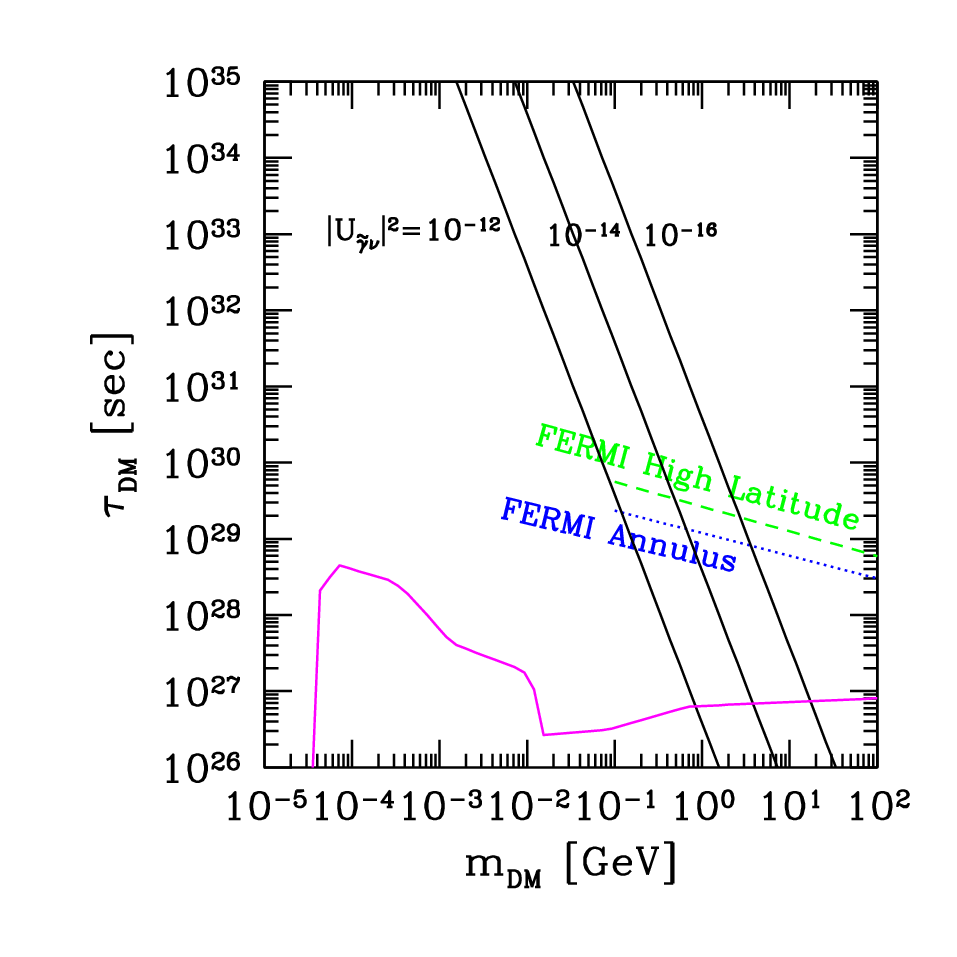There, the decaying dark matter was constrained using the gamma-ray line emission limits from the galactic center region obtained with the SPI spectrometer on INTEGRAL satellite, and the isotropic diffuse photon background as determined from SPI, COMPTEL and EGRET data. These constraints are shown with a magenta line in Fig. 2, where a conservative non-singular profile at the galactic center is used.

On the other hand, the FERMI satellite [23] launched in June 2008 is able to measure gamma rays with energies between 0.1 and 300 GeV. We also show in Fig. 2 the detectability of FERMI in the ’annulus’ and ’high latitude’ regions following the work in [18]. Below the lines, FERMI will be able to detect the signal from decaying dark matter. Obviously, no signal means that the region would be excluded and FERMI would have been used to constrain the decay of dark matter [18].

Finally, we show in the figure with black solid lines the values of the parameters predicted by the $\mu\nu$SSM using Eq. (21), for several representative values of $|U_{\widetilde{\gamma}\nu}|^{2}$. We can see that values of the gravitino mass larger than 20 GeV are disfavored in this model by the isotropic diffuse photon background observations (magenta line). In addition, FERMI will be able to check important regions of the parameter space with gravitino mass between $0.1-20$ GeV and $|U_{\widetilde{\gamma}\nu}|^{2}=10^{-16}-10^{-12}$ (those below the green line).

Let us now discuss in more detail what kind of signal is expected to be observed by FERMI if the gravitino lifetime and mass in the $\mu\nu$SSM (black solid lines) correspond to a point below the green line in Fig. 2

As it is well known, there are two sources for a diffuse background from dark matter decay. One is the cosmological diffuse gamma ray coming from extragalactic regions, and the other is the one coming from the halo of our galaxy.

The photons from cosmological distances are red-shifted during their journey to the observer and the isotropic extragalactic flux turns out to be [14, 28, 18]

with

Here $\kappa=\Omega_{\Lambda}/\Omega_{M}\simeq 3$ with $\Omega_{\Lambda}+\Omega_{M}=1$, $\rho_{c}=1.05\ {h^{2}}\times 10^{-5}\,\textrm{GeV}\,\textrm{cm}^{-3}$, $H_{0}=h\ 100\,\textrm{km}\ s^{-1}\ \,\textrm{Mpc}^{-1}$ with $h=0.73$ [31], and ${\tau_{\textrm{DM}}}$ and ${m_{\textrm{DM}}}$ are the lifetime and mass of the dark matter particle, respectively. We take the dark matter density as $\Omega_{DM}h^{2}=0.1$.

On the other hand, the photon flux from the galactic halo shows an anisotropic sharp line. For decaying dark matter this is given by

with

where the halo dark matter density is integrated along the line of sight, and we will use a NFW profile [32]

where we take $\rho_{h}=0.33\,\textrm{GeV}/\,\textrm{cm}^{3}=0.6\times 10^{5}\rho_{c}$, $r_{c}=20$ kpc, and $r$ is the distance from the center of the galaxy. The latter can be re-expressed using the distance from the Sun, $s$, in units of ${R_{\odot}}=8.5$ kpc (the distance between the Sun and the galactic center) and the galactic coordinates, the longitude, $l$, and the latitude, $b$, as

It is worth noticing here that when computing above the gamma-ray fluxes, the effects of attenuation of the flux in the interstellar or the intergalactic medium have been neglected. In our mass range of the gravitino, the flux from the decay of the gravitino dark matter is made of photons and neutrinos, thus we might expect the attenuation of the gamma-ray flux by pair production. Nevertheless, for our case with less than 10 GeV gamma-ray flux the attenuation is suppressed both in the galactic and extragalactic medium [33], and can therefore be safely neglected.

Let us now compute with the above formula, as an example, the expected diffuse gamma-ray emission in the mid-latitude range ($10^{\,\circ}\leq|b|\leq 20^{\,\circ}$), which is being analized by FERMI [34], for the case of gravitino dark matter. Let us assume for instance a value of $m_{3/2}=3.5\,\textrm{GeV}$ and $\left|U_{\tilde{\gamma}\nu}\right|^{2}=8.8\times 10^{-15}\,(1.7\times 10^{-15})$ in the $\mu\nu$SSM, corresponding to $\tau_{3/2}=10^{27}$ ($5\times 10^{27}$) s, using Fig. 2. We convolve the signal with a Gaussian distribution with the energy resolution $\Delta E/E=0.08$, between $E=1-10\,\textrm{GeV}$, following [23], and then we average the halo signal over the region for the mid-latitude range mentioned above.

The results for the two examples are shown in Fig. 3. There, the green dashed line corresponds to the diffuse extragalactic gamma ray flux, and the magenta solid line corresponds to the gamma-ray flux from the halo. The black solid lines represent the background including the diffuse galactic emission model from GALPROP [35], and point source and isotropic contributions [34]. The systematic uncertainties for the latter generate the band shown within the two black lines.

The total gamma-ray flux, including background, extragalactic, and line signal, is shown with red solid lines. We can see that the sharp line signal associated to an energy half of the gravitino mass, dominates the extragalactic signal and can be a direct measurement (or exclusion) in the FERMI gamma ray observation. We could also use the EGRET data [36] to constrain the parameter space of the model. Although the data beyond 1 GeV are controversial (even instrumental effects might be a possible explanation for the observed excess [37]), the line obtained in the example of Fig. 3a is very sharp and could be discarded when compared with the spectrum of EGRET.

As another example, we show in Fig. 4 the case of $m_{3/2}=10$ GeV for the same values of lifetimes as in Fig. 3.

We have discussed the possibility of gravitino dark matter in the $\mu\nu$SSM, where R-parity is broken and therefore the LSP is unstable. For the gravitino mass of the order of  GeV, the lifetime of the gravitino is much longer than the age of the Universe and the observed relic density can be explained well by the thermal production of gravitinos after inflation. As a consequence, the gravitino can be a good candidate for dark matter.

We have also studied the prospects for detecting gamma rays from decaying gravitinos. If the gravitino explains the whole dark matter component, the gravitino mass larger than $20\,\textrm{GeV}$ is disfavored by the isotropic diffuse photon background measurements. Nevertheless, a gravitino with a mass range between $0.1-20$ GeV gives rise to a signal that might be observed by the FERMI satellite. In this way important regions of the parameter space of the $\mu\nu$SSM can be checked.

After completion of the current work, the FERMI experiment reported 5-month measurements of the diffuse gamma-ray emission in the mid-latitude range [38]. We have added in Figs. 3 and 4 blue solid lines corresponding to these Fermi LAT data with systematic uncertainties. These turn out to be consistent with the background model, implying that the sharp lines obtained in the examples of Figs. 3a and 4a have not been observed. Taking these results into account, we have summarized in Fig. 5 the constraints on lifetime versus mass for the $\mu\nu$SSM. Values of the gravitino mass larger than 10 GeV are now disfavored, as well as lifetimes smaller than about 3 to 5$\times 10^{27}$ s.

We gratefully acknowledge G. Bertone for his collaboration during the early stages of this work. We thank A. Morselli for very helpful information concerning FERMI. We also thank G.A. Gómez for his valuable comments. The work of the authors was supported by the spanish MICINN’s Consolider-Ingenio 2010 Programme under grant MULTIDARK CSD2009-00064. The work of K.Y. Choi and C. Muñoz was supported in part by MICINN under grants FPA2009-08958 and FPA2009-09017, by the Comunidad de Madrid under grant HEPHACOS S2009/ESP-1473, and by the European Union under the Marie Curie-ITN program PITN-GA-2009-237920. D.E. López-Fogliani thanks STFC for financial support. The work of R. Ruiz de Austri was supported in part by MICINN under grant FPA2007-60323, by the Generalitat Valenciana under grant PROMETEO/2008/069, and by the Spanish Consolider-Ingenio 2010 Programme CPAN (CSD2007-00042). We also thank the ENTApP Network of the ILIAS project RII3-CT-2004-506222 and the UniverseNet Network MRTN-CT-2006-035863.

References

- [1] D. E. López-Fogliani and C. Muñoz, Phys. Rev. Lett. 97 (2006) 041801 [arXiv:hep-ph/0508297].
- [2] N. Escudero, D. E. Lopez-Fogliani, C. Muñoz and R. R. de Austri, JHEP 12 (2008) 099 [arXiv:0810.1507 [hep-ph]].
- [3] C. Muñoz, unpublished notes (1994).
- [4] J. E. Kim and H. P. Nilles, Phys. Lett. B138 (1984) 150.
- [5] For a review, see e.g.: U. Ellwanger, C. Hugonie and A.M. Teixeira, arXiv:0910.1785[hep-ph], and references therein.
- [6] D.J.H. Chung and A. Long, in preparation; A. Long, talk at Phenomenology 2009 Symposium - PHENO 09, 11-13 May, Madison, Wisconsin, USA.
- [7] For a review, see: H.K. Dreiner, in the book ’Perspectives on supersymmetry’, World Scientific, p. 462 [arXiv:hep-ph/9707435].
- [8] J.A. Casas, E.K. Katehou and C. Muñoz, Oxford preprint, Nov. 1987, Ref: 1/88; Nucl. Phys. B317 (1989) 171; J.A. Casas and C. Muñoz, Phys. Lett. B212 (1988) 343 [arXiv:hep-ph/0309346].
- [9] P. Ghosh and S. Roy, JHEP 0904 (2009) 069 [arXiv:0812.0084 [hep-ph]].
- [10] A. Bartl, M. Hirsch, A. Vicente, S. Liebler and W. Porod, JHEP 0905 (2009) 120 [arXiv:0903.3596 [hep-ph]].
- [11] J. Fidalgo, D. E. López-Fogliani, C. Muñoz and R. R. de Austri, JHEP 08 (2009) 105 [arXiv:0904.3112[hep-ph]].
- [12] For a review, see e.g.: C. Muñoz, Int. J. Mod. Phys. A19 (2004) 3093 [arXiv:hep-ph/0309346].
- [13] See e.g.: D.G. Cerdeño, C. Muñoz and O. Seto, Phys. Rev. D79 (2009) 023510 [arXiv:0807.3029 [hep-ph]], and references therein.
- [14] F. Takayama and M. Yamaguchi, Phys. Lett. B485 (2000) 388 [arXiv:hep-ph/0005214].
- [15] M. Hirsch, W. Porod and D. Restrepo, JHEP 03 (2005) 062 [arXiv:hep-ph/0503059].
- [16] W. Buchmuller, L. Covi, K. Hamaguchi, A. Ibarra and T. Yanagida, JHEP 03 (2007) 037 [arXiv:hep-ph/0702184].
- [17] S. Lola, P. Osland and A. R. Raklev, Phys. Lett. B656 (2007) 83 [arXiv:0707.2510 [hep-ph]].
- [18] G. Bertone, W. Buchmuller, L. Covi and A. Ibarra, JCAP 11 (2007) 003 [arXiv:0709.2299 [astro-ph]].
- [19] A. Ibarra and D. Tran, Phys. Rev. Lett. 100 (2008) 061301 [arXiv:0709.4593 [astro-ph]].
- [20] A. Ibarra and D. Tran, JCAP 07 (2008) 002 [arXiv:0804.4596 [astro-ph]].
- [21] K. Ishiwata, S. Matsumoto and T. Moroi, Phys. Rev. D78 (2008) 063505 [arXiv:0805.1133 [hep-ph]].
- [22] L. Covi, M. Grefe, A. Ibarra and D. Tran, JCAP 01 (2009) 029 [arXiv:0809.5030 [hep-ph]].
- [23] W. B. Atwood et al. [FERMI/LAT Collaboration], Astrophys. J. 697 (2009) 1071 [arXiv:0902.1089 [astro-ph.IM]].
- [24] D.N. Spergel et al. [WMAP Collaboration], Astrophys. J. Suppl. 148 (2003) 175 [arXiv:astro-ph/0302209].
- [25] M. Bolz, A. Brandenburg and W. Buchmuller, Nucl. Phys. B606 (2001) 518 [Erratum-ibid. B790 (2008) 336] [arXiv:hep-ph/0012052].
- [26] M. Viel, J. Lesgourgues, M. G. Haehnelt, S. Matarrese and A. Riotto, Phys. Rev. D71 (2005) 063534 [arXiv:astro-ph/0501562]; M. Viel, G. D. Becker, J. S. Bolton, M. G. Haehnelt, M. Rauch and W. L. W. Sargent, Phys. Rev. Lett. 100 (2008) 041304 [arXiv:0709.0131 [astro-ph]].
- [27] G.L. Fogli, E. Lisi, A. Marrone, A. Melchiorri, A. Palazzo, A. M. Rotunno, P. Serra, J. Silk and A. Slosar, Phys. Rev. D78 (2008) 033010 [arXiv:0805.2517 [hep-ph]].
- [28] J. M. Overduin and P. S. Wesson, Phys. Rept. 402, 267 (2004) [arXiv:astro-ph/0407207].
- [29] H. Yuksel and M. D. Kistler, Phys. Rev. D78 (2008) 023502 [arXiv:0711.2906 [astro-ph]].
- [30] S. Palomares-Ruiz, Phys. Lett. B665 (2008) 50 [arXiv:0712.1937 [astro-ph]].
- [31] W. M. Yao et al. [Particle Data Group], J. Phys. G33 (2006) 1.
- [32] J.F. Navarro, C.S. Frenk and S.D.M. White, Astrophys. J. 462 (1996) 563.
- [33] F.W. Stecker, M.A. Malkan and S.T. Scully Astrophys. J. 648 (2006) 774 [arXiv:astro-ph/0510449], Astrophys. J. 658 (2007) 1392 [arXiv:astro-ph/0612048]; I.V. Moskalenko, T.A. Porter and A.W. Strong, Astrophys. J. 640 (2006) L155 [arXiv:astro-ph/0511149]; A. Ibarra, D. Tran and C. Weniger, arXiv:0909.3514[hep-ph].
- [34] A. Morselli, talk at the 5th International Workshop on the Dark Side of the Universe (DSU09), Melbourne, 1-5 June 2009.
- [35]
A.W. Strong and I.V. Moskalenko, Astrophys. J. 509 (1998) 212;
The code and documentation is available at
http://galprop.standford.edu/web-galprop/galprop-home.html - [36] S.D. Hunter et al., Astrophys. J. 481 (1997) 205.
- [37] I.V. Moskalenko et al., Nucl. Phys. B Proc. Supp. 173 (2007) 44.
- [38] A.A. Abdo et al. [FERMI/LAT Collaboration], Phys. Rev. Lett. 103 (2009) 251101 [arXiv:0912.0973 [astro-ph.HE]].