HQP08
MZ-TH/09-21 Radiative corrections to top quark decays
Abstract
We provide a pedagogical introduction to the subject of Standard Model decays of unpolarized top quarks into unpolarized and polarized -bosons including their QCD and electroweak radiative corrections.
1 Introductory remarks
These lectures held by one of us (JGK) at the II Helmholtz International Summer School on Heavy Quark Physics in Dubna, Russia (August 11 - 21 2008) are meant as pedagogical lectures aimed at the level of the audience which, on the participants’ side, was composed of graduate students with a few postdoctoral students mixed in. We give many details on the Born level calculation of rates and angular decay distributions which can be profitably used in the higher order radiative correction calculations. The material collected in the write-up of the lectures given by one of us at the International School on Heavy Quark Physics in Dubna, Russia (27 May - 5 Jun 2002) [1] covering similar topics will not always be repeated. In addition to the review [1] we very much recommend the excellent reviews on top quark physics in [2, 3, 4, 5, 6]. One of the main aim of these lectures is to illustrate advanced loop techniques in simple Born term settings. We begin by listing the basic properties of the Standard Model (SM) top quark and its SM decay features.
1.1 Mass of the top quark
In our numerical calculations we always take the top quark mass to be GeV. The latest Tevatron combination is GeV [7]. Since all our results are in closed analytical form any other value of the top quark mass can be used as input in these formulas.
There have been suggestions for indirect measurements of the top quark mass through the measurements of dynamic quantities that depend on the value of the top quark mass. For example, the SM -production rate at e.g. hadron colliders is sensitive to the value of the top quark mass (in particular at the Tevatron II) and thus the -production rate could be used to “measure” the top quark mass. Another possibility is to accurately measure the longitudinal and transverse-minus helicity decay rates of the top quark. The ratio of the two helicity rates is well suited for an indirect determination of the top quark mass since the ratio depends quadratically on the top quark mass, i.e. . One should, however, always take into account radiative corrections in such indirect top quark mass measurements. For example, in the latter case the NLO QCD and electroweak radiative corrections have different effects on the two partial helicity rates which lead to a upward shift in the helicity rate ratio for top quark masses around 175 GeV [8, 9].
In a third method one measures the mean distance that -hadrons from -events travel before they decay [10]. The mean distance is obviously correlated with the value of the top quark mass. Needless to say that all these indirect top quark mass measurements crucially depend on the assumed correctness of the SM.
1.2 Top quark decays before it can hadronize
Singly produced top quarks in hadronic collisions are produced by weak interactions and are almost 100% polarized. The top quark retains its polarization which it has at birth when it decays. The standard argument is that the life time of the top quark () is shorter than the hadronization time which is characterized by the inverse of the nonperturbative scale of QCD, i.e..
However, one can do better as pointed out in [11] who extended earlier work on depolarization effects in the bottom sector [12, 13]. Consider a polarized top quark which picks up a s-wave light antiquark of opposite spin direction. This state will be a coherent superposition of the spin 0 and spin 1 mesonic ground states as follows
| (1) |
The coherent superposition will become decoherent on two counts. First the system oscillates between the two mass eigenstates with a time scale characterized by the mass difference where . Loss of coherence through the decay can be neglected since it sets in much later at a time scale [11]. Thus the depolarization time scale is set by and is larger than the tradional estimate based on by a factor of 60. Altogether, the top quark has decayed after much before depolarization sets in at . One concludes that the top quark retains its polarization which it has at birth when it decays.
The decay of polarized top quarks and the corresponding spin-momentum correlations in these decays will not be discussed in these lectures. A discussion of the spin-momentum correlations and their NLO QCD corrections can be found in [8, 14, 15]. We mention that top quarks produced at -colliders also possess a high degree of polarization which, in addition, can also be attuned by tuning the beam polarization.
The issue of whether the top quark retains its original polarization when it decays is also of importance in the case of hadronically produced top quark pairs. Although the single top (or antitop) polarization is zero because parity is conserved in the hadronic production process there are sizable spin-spin correlations of the top and antitop quark spins which give important information on the -production process (see e.g. [4]).
1.3 Dominance of the decay
From the unitarity of the KM–matrix one has the relation
| (2) |
One concludes that . There are a number of other SM decays such as which are negligible compared to the dominant mode 11 1 In order to simplify the notation we shall in the following refer to the decay as ..
1.4 Rate ratio of and
Let us list the possible leptonic and hadronic decay modes of the the . For the leptonic modes one has the three modes
| (3) |
When listing the weight factor we have neglected lepton mass effects.
For the hadronic modes one has
| (4) | |||||
Again mass effects have been neglected. In (4) we have summed over the respective three modes using again the unitarity of the KM-matrix and . In addition one has to add in a factor of three from colour summation. One thus obtains
| (5) |
1.5 Width of the top quark
As mentioned before the top quark decays almost 100% to in the SM. The other SM decay modes are negligible. Let us list the theoretical values of the SM decay width and radiative corrections relative to the Born term width ( GeV for ).
| Born LO | ||||||
| QCD NLO [16] | ||||||
| electroweak NLO [17, 18] | ||||||
| QCD NNLO [19, 20] | (6) |
The NLO and NNLO QCD corrections and the NLO electroweak corections will be discussed in Sec. 2. The finite width corrections will be discussed in Sec. 5.
It is interesting to note that the non-SM decay width into a charged Higgs can become comparable in size to the SM decay width for small and large values of if is not too close to the phase space boundary (see e.g. [4]). A precise measurement of the top quark decay width could therefore provide stringent exclusion regions in the ()-parameter space of Two-Higgs-Doublet models which contain a charged Higgs boson.
The measurement of the top quark decay width is not simple at hadron colliders. In principle there are two methods to experimentally get a handle on the decay width or lifetime of the top quark. One can attempt to measure the mean decay length in the laboratory which is given by the mean decay length 22 2 We have employed a mixed notation in the last equality of Eq.(7) where we set for the quantities in the square bracket .
| (7) |
where and , and and . That this measurement is difficult is illustrated by the following example. Take a top quark width of 1.43 GeV. The laboratory momentum of the top quark must have the astronomically high value of GeV to produce a mean decay length of 1mm. Nevertheless CDF has attempted such a measurement using information on the magnitude of the impact parameter of the charged lepton with respect to the collision vertex. CDF puts a 95% confidence level upper limit of on the lifetime of the top quark which corresponds to a GeV lower limit on the top quark width [21]. Naturally, this is not a very useful bound. CDF also provides an upper limit on the top quark width by a fit of the reconstructed top quark mass to a Breit-Wigner shape function. The reult is GeV at 95% C.L. [22]. The upper bound is still nine times larger than the expected SM width.
An indirect way of determining the top quark width relies heavily on the validity of the SM. The suggestion is to measure the branching ratio . This could be done e.g. by measuring the rate of top quark pair production followed by their decays , i.e. by measuring . Assuming that one can reliably calculate one can then extract (see e.g. [3]). In the simplest version of this approach one takes the SM value to determine the width of the top quark through . In a more sophisticated approach one uses single-top production to extract the parameters that determine the partial width [23].
We mention that a much improved determination of the top quark width with an uncertainty of MeV can be expected from a multi-parameter scan of the threshold region of -production at the ILC [24].
1.6 Top quark yield
At the LHC top quark pairs will be produced quite copiously in 7 on 7 TeV proton-proton collisions. After a one-year probation run at reduced energies and luminosities starting in the end of 2009 the LHC will start running at full energy in 2010 with a low luminosity run of . After a luminosity upgrade around the year 2017 the high luminosity run will have . Multiply these numbers with to obtain -pairs every second for the low (high) luminosity run.
Top quark pair production at the Tevatron II (1 on 1 TeV -collisions) occurs at a reduced rate. Because the energy of the Tevatron II is lower, the -production cross section is down by a factor of . In addition, the Tevatron II luminosity is down by a factor of compared to the LHC low luminosity run. Taking these two factors into account one has -pairs per second at the Tevatron II.
In the SM single top production cross section in - and -collisions is down by a factor of compared to top quark pair production. The nice feature of single top production is that the top quarks are polarized since the production of single top quarks proceeds through weak interactions. The polarization can be calculated to be close to 100% (see e.g. [4]).
1.7 Polarization of gauge boson
The decay is weak and therefore the -boson is in general expected to be polarized. We shall refer to the three partial rates that correspond to the three polarization states of the -boson as longitudinal , transverse-plus and transverse-minus . At leading order (LO) the results for the helicity fractions (or, in another language, for the normalized diagonal density matrix elements of the -boson , and ) are33 3 The helicities of the -boson are alternatively labelled by , or by .
| (8) |
where with . Numerically one has
| (9) |
Note that . In comparison, an unpolarized would correspond to
| (10) |
1.8 Dominance of the longitudinal mode
As the longitudinal polarization vector becomes increasingly parallel to (see e.g. [1]), viz.
| (11) |
Therefore the longitudinal mode dominates in the large top quark mass limit. In fact, from one concludes from dimensional arguments that whereas or .
An explicit calculation shows that at LO for (see Eq.(8)). Looking at Fig. 1 the vanishing of the LO transverse-plus rate can be understood from angular momentum conservation. First remember that a massless left-chiral fermion is left-handed as drawn in Fig. 1. At LO one has a back-to-back decay configuration. Therefore the -boson cannot be right-handed because the -quantum numbers in the final state would add up to which cannot be reached by the spin 1/2 top quark in the initial state. At NLO (or any higher order) the decay is, in general, no longer back-to-back as illustrated in Fig. 1 and one anticipates that at NLO and at any higher order. This is, in fact borne out by the NLO calculation to be described later on. The physics interest lies in the fact that nonvanishing transverse-plus helicity rates can also be generated by non-SM right-chiral ()-currents. In order to unambigously identify non-SM contributions to the transverse-plus helicity rate it is therefore important to get a quantitative handle on the size of the SM higher order radiative correction contributions to the transverse-plus helicity rate.

1.9 Measurement of the helicity fractions of the through the angular decay distribution in its decay
The decays weakly to or to . The angular decay distribution can therefore be utilized to analyze the polarization of the decaying , i.e. the is self-analyzing.
The has the three (diagonal) polarization states , and the weights of which are determined by the three partial helicity rates and . As we shall explicitly derive further on, the angular decay distribution for reads

| (12) |
where the polar angle is measured in the –rest frame as shown in Fig. 2. Integrating over one recovers the total rate . If the were unpolarized one would have resulting in a flat decay distribution .
One can also define a forward-backward asymmetry by considering the rate in the forward hemisphere and in the backward hemisphere in the -rest frame. The forward-backward asymmetry is then given by
| (13) |
At the Born term level one has
| (14) |
The forward-backward asymmetry is negative, i.e. one has more leptons in the backward hemisphere than in the forward hemisphere. The numerical value of the forward-backward asymmetry is not very large on account of the dominance of the longitudinal mode.
It is always useful to check on the correctness of the sign of the parity violating term proportional to () and thereby on the sign of . This is again easily done by considering the collinear cases and appealing to angular momentum conservation. And, in fact, Eq.(12) shows that the mode decouples in the forward direction (and vice versa decouples in the backward direction) as can be appreciated from the helicity configurations in Fig. 2. This implies that favours forward leptons leading to energetic leptons in the -rest frame whereas favours backward leading to less energetic leptons in the -rest frame. As we have seen at LO so that one expects a softer lepton spectrum in the -rest frame then in the case of the decay of an unpolarized .
2 Top quark decay rate
2.1 Leading (LO) rate
We shall calculate the leading order rate in three different ways for pedagogical reasons. The first way is the traditional covariant way where no particular sophistication is needed. In the second way we use the helicity methods which has the advantage that by calculating the helicity amplitudes one has the full spin information of the decay at hand. In the third method we use the optical theorem which serves the purpose of introducing rather sophisticated technical material in a simple setting which are needed later on in the higher order calculations.
2.1.1 Covariant method
The matrix element for the decay is given by
| (15) |
Upon squaring and summing over the spins one obtains
| (16) |
where we write . Use of the completeness relations
| (17) |
and
| (18) |
leads to
| (19) |
Using four-momentum conservation and the mass shell conditions and one obtains
The rate can be computed using the two–body decay formula
| (20) |
where denotes the two-body phase space integral [27]. We symbolically write for the two-body phase space integration over the squared matrix element , i.e. we write
| (21) |
In order to stay general we calculate for . The phase space integral will be evaluated in the top quark rest system. We write , where we implicitly take the positive energy solution . The corresponding relation for the bottom quark energy reads . Using these two relations one converts the three-dimensional integrations in (21) into four-dimensional integrations. One obtains
| (22) |
The integration over can be done with the result that the argument of the second -function becomes , i.e.
| (23) |
Next one integrates over with the result that the argument of the remaining -function becomes . The remaining integration over can be done using spherical coordinates such that . The result is
| (24) |
where is the magnitude of the momentum of the -boson in the top quark rest (–rest) frame and where is Källén’s function. Naturally we could have calculated the two-body phase space directly without including the squared matrix element in the integrand as long as the kinematic variables in are fixed according to four-momentum conservation and the mass-shell conditions.
We now return to the approximation where . Substituting the matrix element squared (19) into the rate formula (20) one obtains
| (25) |
where is the Born term rate ()
| (26) |
2.1.2 Helicity amplitude method
The helicity amplitudes for can be calculated from the transition matrix element by using spinors and polarization vectors with definite helicities and . One needs to calculate (we omit the coupling factor )
| (27) |
We shall work in the –rest system with the -axis along the (see Fig. 3) such that . In order to be general we keep .

Let us collect the relevant –rest system spinor and polarization vector expressions. For the helicity spinors one has
where are Pauli spinors given by and .
The helicity polarization four-vectors of the read
| (32) |
There are altogether four possible helicity configurations in which are listed in Table 1.
| 1/2 | -1/2 | 0 |
| -1/2 | 1/2 | 0 |
| 1/2 | 1/2 | 1 |
| -1/2 | -1/2 | -1 |
For the helicity amplitudes () one obtains
| (33) |
where we have included both the and results in (33). The squared matrix element finally is given by
| (34) | |||||
where we have set in the second line of (34). The result agrees with the covariant calculation (see Eq.(19)). The advantage of the helicity method is that one can separately identify the three (diagonal) helicity contributions of the boson , and as indicated in Eq.(34). In fact, the helicity amplitudes contain the complete spin information of the process. Thus one can easily calculate other polarization effects using the helicity amplitudes such as the decay of polarized top quarks, the polarization of the bottom quark and polarization correlation effects. effects are easily included by using the helicity amplitudes in Eq.(33). One can also define covariant helicity projectors which allow one to directly calculate the longitudinal, the transverse-plus and transverse-minus helicity rates without taking recourse to the helicity amplitudes. This will be described in Sec. 5.
2.1.3 Optical theorem method and cutting rules
In this subsection we shall use yet another method to calculate the leading order rate for using the optical theorem. Whereas the optical theorem method does not offer particular technical advantages in LO calculations it is the method of choice for higher order calculations as e.g. the calculation of the NNLO rate to be described later on. The reason is simply that the phase space integrations in the NNLO radiative correction calculations become prohibitively complicated and cannot be automated as easily as higher order loop calculations. We present the optical theorem method for the LO case for pedagogical reasons because the LO discussion allows us to introduce concepts which are also needed in the NNLO radiative correction calculation to be described later on.

The optical theorem relates the width of a particle to the imaginary part of the self-energy contribution of the particle. In the top quark case one has 44 4 A very nice discussion of the optical theorem and related technical material relevant to top quark decays can be found in the thesis of I.R. Blokland [28].
| (35) |
where, for the present purposes, is the one-loop self-energy of the top quark as illustrated in Fig.4.
Using standard Feynman rules [27, 28] the one-loop self-energy contribution is given by
| (36) | |||||
One can again use the completeness relation to rewrite Eq.(36) as a trace. The trace can be taken as in Eq.(19) except that one now cannot avail of the mass-shell conditions and . One obtains
| (37) |
The usual procedure is to expand the -dependent numerator factors in terms of the -dependent denominator factors and in order to obtain -independent numerator factors (the corresponding integrals are called scalar integrals) after cancellation. We therefore write
| (38) |
The contributions proportional to and cancel against the denominator pole factors and their contributions can be dropped when taking the imaginary part since single or zero pole contributions have no imaginary part (see e.g. [28]). We therefore have
| (39) |
According to the cutting rules the discontinuity of a Feynman graph is obtained by the product of the discontinuities of the pole factors which are being cut, where the discontinuity of a single pole is given by [27, 28]
| (40) |
Furthermore, the imaginary part and the discontinuity of a graph are related by . One therefore has
| (41) |
In order to exhibit the similarity to the integral (23) we change the integration variable . One can then use the result of Sec. 2.1.1
to arrive at
| (42) |
where, as before,
| (43) |
As it must be the result agrees with the covariant and helicity amplitude calculations. It is quite reassuring that the decay rate turns out to be positive definite in the end, as it must be, considering all the minus signs and the factors of (i) appearing in the rate calculation using the optical theorem method.
2.1.4 Expansion by regions and the -expansion
In Sec 2.1.3 we have calculated the leading order rate by using the optical theorem and cutting rules to determine the imaginary part of the one-loop self energy diagram. In this subsection we shall go one step further and calculate the leading order rate using a -expansion which allows us to introduce the concepts of expansion by regions and integration-by-parts identities. All latter three concepts are essential in the calculation of the NLLO rate presented in [19, 20]. As emphasized before we shall pattern the LO rate calculation after the NNLO calculation entirely for pedagogical reasons. In the LO case the follow-up calculations are simple enough to be presented in a few simple lines, whereas they are more involved in the full NNLO calculation.
Let us summarize the main ideas of the NNLO rate calculation presented in [19, 20] which we down-size to the present LO case.
- •
Reduce the two-mass-scale problem to a one-mass-scale problem by expanding in the ratio . Obtain the results as an expansion in powers of .
- •
Use dimensional regularization to regularize the UV and IR/M singularities
- •
One has to consider the two regions [29, 30, 31]:
- •
Hard region
The loop momentum is hard and is of . One can then expand the -propagator as a power series in :(44) The massive propagator has thereby been converted into a sum of massless propagators.
- •
Soft region
The momentum q flowing through the is soft. One therefore cannot use the above expansion (44) of the propagator. However, in the soft region one can expand the -quark propagator, cif.(45) There is only one denominator factor in the loop integral and its imaginary part vanishes
(46) Therefore there is no contribution from the soft region in the one-loop case. This is different at NLO and NNLO.
What remains to be done is to evaluate integrals of the form
| (47) |
which result from the expansion in the hard region. The integrals can all be reduced to one master integral by using integration-by-parts identities.
The first term in the expansion (44), , leads to a two–point one–loop integral of the form
| (48) |
We calculate the one-loop integral directly in dimensional regularization and take its imaginary part at the end without resorting to the cutting rules. The details of how to evaluate one-loop integrals in dimensional regularization can be found in [27]. One first introduces a one parameter Feynman parametrization, collects terms and performs a shift in the integration variable , i.e.
| (49) | |||||
Next we do a Wick rotation . The factor of from the Wick rotation cancels the factor of in the denominator of (47). One then does a D-dimensional Euclidean integration over the loop momentum , and, finally, one integrates over the Feynman parameter which results in Euler’s Beta function . The sequence of steps is represented in the following sequence of equations:
| (50) | |||||
We retain only the finite term in the last line of (50). One obtains
| (51) |
We have used
| (52) |
which leads to
| (53) |
In addition to the integral (48) with the imaginary part of which we have just calculated we also need the imaginary parts of the integrals (47) with . They can be obtained from the “master integral” (48) by integration-by-parts (IBP) techniques [32, 33]. The general procedure of reducing a set of integrals to a set of simpler integrals is called “reduction to master integrals”. In the present case this reduction is quite trivial but can become quite involved in more general settings. The reduction procedure has been automated by the Laporta algorithm [34, 35].
Technical aside: Integration-by-parts (IBP) identities [32, 33].
In order to calculate the integral corresponding to the second term in the
expansion (44) we consider the differential form
()
| (54) |
Differentiate carefully, i.e. , and drop the “surface term” on the left-hand side. Also use . This gives
| (55) |
In dimensional regularization massless tadpole (single pole) diagrams are zero, i.e. one can drop the second term on the r.h.s. of (55) after dimensional integration. At the relevant order of one therefore has
| (56) |
Going through the same exercise for for one finds
| (57) |
Because the higher order terms vanish we only need to sum the first two terms in the expansion (44). The result
| (58) |
is in agreement with the one in Sec. 2.1.3.
2.2 Next-to-leading order (NLO) QCD corrections
The traditional technique used for NLO calculation is to calculate the one-loop and tree-graph contributions separately. In the present case the UV singularities are regularized by dimensional regularization whereas the IR/M singularities are regularized by introducing gluon and bottom quark masses. The IR/M singularities will eventually appear as and singularities and cancel among the one-loop and tree graph contributions [8, 9, 14, 16, 36]. We mention that the calculation can also be done in dimensional regularization without recourse to the traditional and regularization [37].
For example, generic diagrams for the QCD NLO calculation are displayed in Fig. 5.


Without going into the details of the calculation (see e.g. [8]) we just quote the result of the NLO calculation. For the total rate one obtains () (see e.g. [36])
| (59) | |||||
The numerical value of the NLO QCD correction appears in Eq.(6). Our numerical input values are GeV and GeV. The strong coupling constant has been evolved from to using two-loop running. Numerically one has . One sees that the NLO QCD corrections reduce the Born term rate by the large amount of .
In the limit one obtains
| (60) |
The leading contribution reduces the rate by which is already quite close to the rate reduction of the full result (). We shall return to an assessment of the quality of the -expansion later on. It is curious to note that the radiative QCD corrections reduce the LO rate whereas the radiative QCD corrections to the decay enhance the LO rate ratio by , i.e. .
The NLO rate can also be calculated by the optical theorem method using the -expansion. At NLO one has contributions both from the soft and the hard region leading to an infinite power series in and where the -contributions come from the interplay of the soft and hard integration regions. The results of the -expansion have been checked against the exact result Eq.(59) up to [38] (see also [28]).
2.3 NLO electroweak corrections
In Fig. 6 we have drawn the LO diagram and the four NLO tree-level diagrams that contribute to . We use the Feynman-’tHooft gauge so that one has a NLO contribution from the charged unphysical Higgs boson as shown in Fig. 6. Compare the number of four electroweak NLO tree-level diagrams with the two QCD NLO tree-level diagrams. When squaring the tree-level diagrams one would expect a four-fold complexity factor when going from QCD to the electroweak tree-graph corrections. It is therefore quite remarkable that the squared tree graph expressions in both cases are similar in length and structure [9].


In addition to the tree graph contributions one has to consider 18 three-point one-loop graphs in the Feynman-’tHooft gauge as shown in Fig. 7. Looking at Fig. 7 one would superficially expect 4+8+8=20 one-loop contributions. However, since there is no –vertex, this number reduces to 18 as stated before. In Fig. 7 and are the charged and neutral unphysical Goldstone bosons, and is the physical Higgs. The results of calculating the one-loop contributions exist in amplitude form [17]. In the course of calculating the electroweak radiative corrections to the partial helicity rates the results of [17] were recalculated and confirmed by us. In particular we checked the results of [17] numerically with the automated loop calculation program XLOOPS/GiNaC developed at the University of Mainz [39, 40, 41]. In addition to the one-loop three-point functions one has a large number of one-loop two-point functions needed in the one-loop renormalization program. Again these have been reevaluated using XLOOPS/GiNaC.
We have used the so-called –renormalization scheme for the electroweak corrections where , and are used as input parameters. The –scheme is the appropiate renormalization scheme for processes with mass scales that are much larger than as in the present case. The electroweak radiative corrections are substantially larger in the so-called –scheme where , and are used as input parameters. The numerical results of the electroweak corrections to the rate are given in Eq.(6).
2.4 NNLO QCD corrections
In the NNLO case squaring of the contributing tree and loop diagrams leads to the four generic contributions shown in Fig. 8.

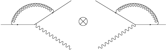


However, with present techniques, this method is not viable, mainly because the NNLO phase space integration become too difficult.
Instead, one resorts again to the optical theorem and calculates the NNLO rate from the three-loop self-energy diagrams according to [19, 20]
| (61) |
There are altogether 38 three-loop Feynman diagrams a sample of which are shown in Fig. 9.

The main ideas of the NNLO calculation of the rate have already been described in the calculation of the Born term rate in Sec. 2.1.3. It turns out that again one only has to consider two momentum regions. In the hard region all loop momenta are hard and the -propagator can be expanded into a series of massless propagators as in the LO case. In the soft region the gluon momenta are hard but the loop momentum flowing through the is soft. Differing from the LO calculation one now also has contributions from the soft region. In the soft region the integrals factorize into two-loop self-energy-type integrals and a one-loop vacuum bubble diagram which are not difficult to integrate. The interplay of the hard and the soft region leads to additional -terms in the -expansion.
One can reduce all integrals to 23 master integrals by integration-by-parts identities. Use was made of Laporta’s algorithm in this reduction to master integrals. The imaginary parts of the master integrals were calculated using the cutting rules where care had to be taken that some of the master integrals admitted several ways of cutting them. We mention that the calculation had been done in the general covariant gauge for the gluon in order to check on gauge invariance. The numerical results on the NNLO QCD corrections are given in Eq.(6).
3 -helicity fractions in top quark decays
3.1 Angular decay distribution for
In Fig. 6 we display the LO amplitude contribution to . On squaring the amplitude and taking the spin sums one is led to the contraction .

For the lepton tensor we obtain
| (62) |
The LO hadron tensor is given by
| (63) |
The factors have been introduced for convenience. The result of contracting the lepton and hadron tensor reads
| (64) |
Note that one originally had
| (65) |
which turns into in the zero lepton mass case where . The lepton mass corrections are of and are thus negligible. If one wants to include lepton mass effects one has to retain the full –projector in (65).
One must evaluate the invariant in one frame. Here we choose the rest frame of the top quark. Since we want to evaluate in terms of the angle defined in the -rest frame () as shown in Fig. 2 we write55 5 In Eq.(66) we have specified the azimuthal dependence of . This is not really needed in the present application because we do not specify a preferred transverse direction. In general, a transverse direction could be defined by the polarization of the top quark or the decay products of the -quark. In this case one has to retain the azimuthal dependence of the lepton’s momentum as done in (66). Whereas the sign of polar angle correlations can always be checked by physics arguments, there are no ready physics arguments to check the signs of the azimuthal correlations. To get the signs of the azimuthal correlations right it is indispensable to use the boosting method as described above (see e.g. [42]).
| (66) |
We then boost the lepton momentum to the top quark rest frame () where the invariants in (64) are to be evaluated. The relevant Lorentz boost matrix reads
| (67) |
such that
The boost will not affect the transverse components but only the zero and longitudinal components . In Eq.(67) and denote the energy and momentum of the -boson in the top quark rest frame.
In the following we set such that and . Boosting one obtains
| (68) |
The remaining momentum four–vectors in the –rest frame are given by
| (69) |
We are now in the position to evaluate the invariants appearing in Eq.(64). We sort the resulting expression in terms of the polar angle factors and . Since we are not interested in the azimuthal angle dependence in the present application we integrate over the azimuthal angle . One then obtains the angular decay distribution
| (70) |
where, by comparison with Eq.(21), we have identified the three LO hadron contributions proportional to and . The normalized helicity fractions and written down before in Eq.(8) can be read off from Eq.(70). As we shall see later on from an angular momentum analysis, the sorting of the angular contributions in (70) should be done exactly along the three angular factors proportional to and discussed above. The corresponding coefficient factors are then proportional to the partial helicity rates and , respectively. An untreated and unsorted Mathematica output of would, in general, lead to quite lengthy and messy expressions.
Repeating the same exercise for one obtains
| (71) |
where
| (72) |
For the normalized helicity fractions one now obtains
| (73) |
where
Let us compare the resulting numerical values for the normalized helicity fraction with their counterparts. One obtains (we take as default value)
| (74) |
The effect of including the nonvanishing bottom quark mass can be seen to be quite small.
Although we have derived the decay distributions (70) and (71) for the Born term case, the angular structure is quite general as will be shown in the next subsection. In the general case one has to replace the LO Born term structure function in (70) and (71) by their generalized counterparts as e.g. the corresponding NLO or NNLO structure functions.
3.2 Angular decay distribution for (II)
The dependence of can also be worked out in a more systematic way by using the completeness relation for the polarization four–vectors Eq.(18) 66 6 Since the method is general we can omit the LO specification in .. One can then rewrite the contraction of the lepton and hadron tensors as
| (75) | |||||
We have thereby converted the invariant contraction into a contraction over the spatial spherical components , where the spatial spherical components of the lepton and hadron tensors are defined by
| (76) |
We have again dropped the -terms in the completeness relation in Eq. (18) since for massless leptons. The nice feature of the representation (75) is that the left bracket and the right bracket in the next to last row of (75) are separately Lorentz invariant. One can therefore evaluate the left bracket in the rest frame, and the right bracket in the –rest system without involving any boost.
Let us now specify the the -rest frame four-vectors that are needed in the -rest frame evaluation of the lepton matrix . In the rest frame one has
| (77) |
and the polarization vectors (in our convention and )
| (78) |
It is then straight-forward to evaluate using the lepton tensor (62).
The various components of the lepton matrix can be written in a very compact and suggestive way in terms of Wigner’s small -function. One has
| (79) |
where the spin one function is given by (convention of Rose)
| (80) |
The rows and columns are labeled in the order . The representation (79) should be of no surprise to anyone who is familiar with the behaviour of angular momentum states under a rotation by the angles and . In the lepton system the only nonvanishing component of the lepton matrix is as the antilepton and the neutrino are both left-handed (see Fig. 2). Eq.(79) represents the rotation of the lepton matrix from the lepton system to the hadron system . In the case one has to augment Eq.(79) by temporal spin components and interference contributions of the temporal spin and spatial spin 1 components [44].
When integrating over the azimuthal angle one remains only with the three diagonal elements of . One has
| (81) |
By convention one drops one of the double indices in the diagonal elements of the hadronic density matrix , i.e. one replaces and as has been done in the rest of this paper. For the LO case one reproduces Eq.(21) using , and from (33).
The advantage of method II is that the method can easily be applied to more complex decay processes involving spin. Also one can easily incorporate lepton mass effects and include polarization effects of initial and final state particles [43, 44]. For example, method II was applied to the full angular analysis of [43, 44] and the rare decays [45] including results on the polarisation of the final lepton. Another example is [42] where we have used method II to describe the semileptonic decay process of a polarized , () followed by the nonleptonic decay . In this process the mass difference is comparable to the –mass which makes inclusion of lepton mass effects mandatory. In fact one finds in this process. A cascade type analysis as used in the method II is ideally suited for Monte Carlo event generators that describe complex cascade decays involving particles with spin. In fact, we wrote a Monte Carlo generator for the above semileptonic decay process [42] which was profitably used in the analysis of the NA48 data on this process.
3.3 Experimental results on helicity fractions
An early MC study quotes experimental sensitivities of and for an integrated luminosity of 100 at Tevatron II energies which corresponds to -pairs [46]. Compare this to the NLO QCD changes and to be discussed later on which shows that the radiative corrections are of the same order as the experimental sensitivities. Much higher event rates can be reached at the LHC in one year. A more recent MC study based on 10 at the LHC quotes measurement uncertainties of , and [47].
Experimentally, there has been a continuing interest in the measurement of the helicity fractions. Latest measurements are
| (82) |
All of these measurements are well within the SM predictions.
4 Construction of covariant helicity projectors
In Eq.(76) we have defined the helicity structure functions which multiply the angular factors in the angular decay distribution. According to their definition in Eq.(76) the helicity structure functions can be calculated in a frame-dependent way by use of the frame-dependent polarization vectors (32). It is much more convenient to calculate the helicity structure functions covariantly, and, in fact, a covariant projection is indispensable for the NLO and NNLO calculations. The covariantization is achieved by defining covariant helicity projectors which covariantly project onto the helicity structure functions via
| (83) |
This definition holds for any general hadron tensor structure irrespective of the fact that we have dealt only with the Born term hadron tensor up to now. To construct the covariant helicity projectors we start with their representation in terms of the -rest frame polarization vectors (32) according to the definition Eq.(76). One has
| (84) |
In covariantizing the forms it helps to remember that the helicity projectors must be four-transverse to the momentum of the , i.e. they must satisfy
| (85) |
Further, they must satisfy the orthonormality and completeness relations
| (86) | ||||||||
As it turns out the covariant projectors can be constructed from the following three projectors
- •
Projector for the total rate
(87) - •
Projector for the longitudinal helicity rate
(88) - •
Projector for the forward-backward asymmetric helicity rate
(89)
The denominator factor refers to the top quark rest frame. In invariant form the normalization factor is given by . Finally, the three projectors read ()
| (90) |
It is instructive to check that, in the -rest frame or in the -rest frames, the covariant helicity projectors in Eq. (90) reduce to the form (84) in terms of the rest frame polarization vectors (32) and (78), respectively. Note, though, that in the -rest frame the normalization factor in Eqs. (88) and (89) has to be replaced by where is the magnitude of the top quark momentum in the -rest frame.
5 Narrow width approximation
Let us begin with by discussing how to factorize of the three–body rate into the two–body rates and using the narrow width approximation for the -boson. The rate formula for the three body decay reads (see [27])
| (91) |
which we write as
| (92) |
The squared three-body matrix element is given by
| (93) |
where we have introduced the Breit-Wigner line shape to account for the finite width of the –boson. We have also reinstituted the factor of in (93) which was introduced earlier for convenience.
Next we introduce the identity
| (94) |
which can be seen to be true in the rest frame where and . The identity (94) allows one to factorize the three-body phase space integral into the two-body phase space integrals and . One has
| (95) | |||||
The phase space nicely factorizes. But how about the factorization of the squared three–body matrix element ? The matrix element squared also factorizes after angular integration which can be seen by using the relation
| (96) |
which follows from the explicit representation of given in Eq.(79). In fact, one has
| (97) |
The factor provides for the crucial statistical factor in the width formula. Note that the explicit angular integrations over and appearing in (97) are implicit in (95) 77 7 We mention that an alternative derivation of the appearance of the statistical factor 1/3 has been given in [50].. One thus finds
| (98) | |||||
The narrow–width approximation consists in the replacement of the Breit-Wigner line shape by a –function,
| (99) |
Using the narrow-width approximation for the -boson the three-body decay can be seen to factorize,
| (100) | |||||
which is a result which one expects from physical intuition. Incidentally, the derivation of the factorization formula (100) was posed as one of the problems in the 2004 TASI lectures of T. Han [51]. Judging from the contents of this subsection this was not one of his simpler problems.
The numerical value of the finite-width correction to the total width listed in (6) consists of the replacement of by the Breit–Wigner line shape and integrating over ,
| (101) |
where is the width of the -boson ( GeV ).
6 Higher order corrections to helicity fractions
6.1 NLO QCD and electroweak corrections
As in the calculation of the NLO total rate structure function (we call where stands for the “unpolarized transverse”) we have employed the traditional technique when calculating the helicity structure functions and , i.e. we have separately calculated the hadronic loop and tree contributions after contracting them with the relevant projectors .
As mentioned before, the appearance of the normalization factors and in the projectors make the calculation technically more difficult than that for the total rate. For the one-loop contribution the additional normalization factors are of no concern since they appear only as overall factors outside of the one-loop integral. This is different for the phase space integration of the tree-graph contributions where the normalization factors appear under the integral. Typically one of the phase space integrations is over the scaled invariant mass of the bottom quark and the gluon . The normalization factors then appear as overall factors and in the phase space integral, where
| (102) |
The ensuing class of phase space integrals is more general and more difficult than the class of integrals appearing in the total rate calculation. Nevertheless, the phase space integrations can still be done in closed form.
In the limit one finds and thus saturates the total rate (see Eq.(60)) in this limit. This is expected since . Results for the other two NLO QCD helicity rates and can be found in [8, 14, 36]. The NLO electroweak corrections to the helicity rates can be found in [9].
Let us summarize our numerical NLO results on the helicity fractions including also the finite width corrections discussed in Sec.5. We write
| (104) |
As before we normalize the partial rates to the total Born term rate . Thus we write . For the transverse-minus and longitudinal rates we factor out the normalized partial Born rates and write ()
| (105) |
where . Writing the result in this way helps to quickly assess the percentage changes brought about by the various corrections.
Numerically one has
| (106) | |||||
and
| (107) | |||||
It is quite remarkable that the electroweak corrections almost cancel the finite width corrections in both cases.
In the case of the transverse-plus rate the partial Born term rate cannot be factored out because of the fact that is zero. In this case we present our numerical result in the form
| (108) |
One has
| (109) | |||||
Note that the finite width correction to the transverse-plus helicity rate is zero. Numerically the NLO corrections to occur only at the pro mille level. It is save to say that, if top quark decays reveal a violation of the SM left-chiral current structure that exceeds the level, the violations must have a non-SM origin such as e.g. an admixture of a right-chiral current structure in the decay vertex .
6.2 Quality of the –expansion
In order to check on the quality of the -expansion we take the known closed form NLO result (103) for and expand it in powers of and . The expansion of the curly bracket in (103) reads
| (110) |
Note that as the phase space closes at (). In Fig. 7 we show a plot of the -dependence of (in units of ) for different orders of and for the full result. All curves start at for . The full result goes to zero at remembering that . As Fig. 7 shows the quality of the expansion is already quite good at even for large -values.
This raises the hope that such a -expansion can also be usefully employed in other contexts. One could think of possible applications of the NNLO calculation of discussed earlier (which only exists in expanded form) to processes such as
- •
- •
extending over the whole kinematical range in these processes.

The region very close to the upper kinematical limit of given by requires a separate discussion because this region is sensitive to effects. The upper kinematical limit is called the zero recoil point since at this point. For example, at zero recoil one finds
| (111) |
using Eq.(73). The equipartitioned helicity fractions result from the fact that, close to zero recoil, the only surviving transition is the allowed Gamow-Teller –wave transition. However, for one has the zero recoil ratios at (see Eq.(8))
| (112) |
In order to investigate the behaviour of the helicity fractions close to zero recoil, in Fig. 8 we plot the -dependence of the helicity fractions for and with zero recoil values at and , respectively. In the region close to their respective zero recoil points the curves considerably differ from each other. Away from zero recoil the and curves very quickly approach each other. Fig. 8 shows that it is safe to use the approximation for -values below .

6.3 NNLO QCD corrections to helicity fractions
In Sec. 2.4 we have desribed how the total NNLO rate can be calculated in a -expansion using the optical theorem. Two new features appear in the corresponding NNLO calculation of the helicity rates . First there is a parity violating three-loop contribution which is projected out by the projector . One has to deal with the problem of how to treat in the environment of dimensionally regularized loop integrals. We take the prescription of [53] and replace
| (113) |
When using this prescription one needs to add finite three-loop counter terms which are given in [54].
The second new feature is related to the normalization factors and in the three helicity projectors which replace the total rate projector . In the hard region one can expand in inverse powers of the (large) propagator pole factor .
| (114) |
One expands in the propagator pole factor , i.e. where one can replace by since one is cutting through the -line anyhow. One then has
| (115) |
Thus, the additional propagator-like structures from the projectors are transformed into a scalar on-shell propagator with momentum and mass raised to arbitrary, integer powers. This will eventually lead to twelve additional three-loop master integrals next to the master integrals appearing in the total rate calculation of [19, 20] whose imaginary parts can again be calculated in closed analytical form using the cutting rules.
In the soft region one cannot perform an expansion of , since and is of order in the soft region. However, in this region the W boson loop factorizes. Therefore, one only has to replace the usual one-loop vacuum bubble integrals with integrals of the type
| (116) |
with and 1. These integrals are not difficult to evaluate.
7 Summary and conclusions
We have discussed some of the properties of the top quark with an emphasis on the SM decay properties of the top quark. We have defined partial helicity rates into polarized -bosons and have derived the resulting angular decay distribution of . We have described the LO calculation of the partial helicity rates using several methods including also the optical theorem and a -expansion as a preparation for the description of the NNLO calculation of the total rate and the partial helicity rates. We have summarily described the main features of NLO QCD and electroweak corrections to the total width and the partial helicity rates.
We are looking forward to the LHC era with its expected wealth of data on the top quark and its decay properties.
Acknowledgements
We are grateful to M.A. Ivanov and H.G. Sander for helpful discussions. JGK would like to thank A. Czarnecki and J. Piclum for their collaboration on the calculation of the NNLO helicity rates.
References
- [1] J. G. Körner and M. C. Mauser, “One-loop corrections to polarization observables,” Lect. Notes Phys. 647 (2004) 212 [arXiv:hep-ph/0306082].
- [2] J. H. Kühn, “Theory of top quark production and decay,” arXiv:hep-ph/9707321.
- [3] D. Chakraborty, J. Konigsberg and D. L. Rainwater, “Review of top quark physics,” Ann. Rev. Nucl. Part. Sci. 53 (2003) 301
- [4] W. Bernreuther, “Top quark physics at the LHC,” J. Phys. G 35 (2008) 083001 [arXiv:0805.1333 [hep-ph]].
- [5] W. Wagner, “Top-quark physics at the Tevatron,” Nucl. Phys. Proc. Suppl. 183 (2008) 67.
- [6] J. R. Incandela, A. Quadt, W. Wagner and D. Wicke, “Status and Prospects of Top-Quark Physics,” arXiv:0904.2499 [hep-ex].
- [7] Tevatron Electroweak Working Group for the CDF Collaboration and D0 Collaborations, arXiv:0903.2503 [hep-ex].
- [8] M. Fischer, S. Groote, J. G. Körner and M. C. Mauser, Phys. Rev. D 65 (2002) 054036
- [9] H. S. Do, S. Groote, J. G. Körner and M. C. Mauser, Phys. Rev. D 67 (2003) 091501
- [10] C. S. Hill, J. R. Incandela and J. M. Lamb, Phys. Rev. D 71 (2005) 054029
- [11] Y. Grossman and I. Nachshon, JHEP 0807 (2008) 016
- [12] F.E. Close, J.G. Körner, R.J.N. Phillips, D.J. Summers, J. Phys. G 18 (1992) 1716.
- [13] A. F. Falk and M. E. Peskin, Phys. Rev. D 49 (1994) 3320
- [14] M. Fischer, S. Groote, J. G. Körner, M. C. Mauser and B. Lampe, Phys. Lett. B 451 (1999) 406
- [15] S. Groote, W. S. Huo, A. Kadeer and J. G. Körner, Phys. Rev. D 76 (2007) 014012
- [16] M. Jezabek and J. H. Kühn, Nucl. Phys. B 314 (1989) 1.
- [17] A. Denner and T. Sack, Nucl. Phys. B 358 (1991) 46.
- [18] G. Eilam, R. R. Mendel, R. Migneron and A. Soni, Phys. Rev. Lett. 66 (1991) 3105.
- [19] I. R. Blokland, A. Czarnecki, M. Slusarczyk and F. Tkachov, Phys. Rev. Lett. 93 (2004) 062001
- [20] I. R. Blokland, A. Czarnecki, M. Slusarczyk and F. Tkachov, Phys. Rev. D 71 (2005) 054004
- [21] CDF-coll, Conf. Note 8104, available from http://www-cdf.fnal.gov/physics/new/top/top.html
- [22] T. Aaltonen et al. [CDF Collaboration], Phys. Rev. Lett. 102 (2009) 042001
- [23] D. O. Carlson and C. P. Yuan, arXiv:hep-ph/9509208.
- [24] M. Martinez and R. Miquel, Eur. Phys. J. C 27 (2003) 49
- [25] S. Groote, J. G. Körner and M. M. Tung, Z. Phys. C 70 (1996) 281
- [26] S. Groote, J. G. Körner and J. A. Leyva, arXiv:0905.4465 [hep-ph]. [27]
- [27] M. E. Peskin and D. V. Schroeder, Reading, USA: Addison-Wesley (1995) 842 p
- [28] I. R. Blokland, “Multiloop calculations in perturbative quantum field theory,” Alberta University thesis 2004, UMI-NQ-95909
- [29] V. A. Smirnov, Mod. Phys. Lett. A 10 (1995) 1485
- [30] V. A. Smirnov, Phys. Lett. B 394 (1997) 205
- [31] M. Beneke and V. A. Smirnov, Nucl. Phys. B 522 (1998) 321
- [32] F. V. Tkachov, Phys. Lett. B 100 (1981) 65.
- [33] K. G. Chetyrkin and F. V. Tkachov, Nucl. Phys. B 192 (1981) 159.
- [34] S. Laporta and E. Remiddi, Phys. Lett. B 379 (1996) 283
- [35] S. Laporta, Int. J. Mod. Phys. A 15 (2000) 5087
- [36] M. Fischer, S. Groote, J. G. Körner and M. C. Mauser, Phys. Rev. D 63 (2001) 031501
- [37] A. Czarnecki, Phys. Lett. B 252 (1990) 467.
- [38] J. H. Piclum, A. Czarnecki and J. G. Körner, Nucl. Phys. Proc. Suppl. 183 (2008) 48.
- [39] A. Frink, J. G. Körner and J. B. Tausk, “Massive two-loop integrals and Higgs physics,” arXiv:hep-ph/9709490.
- [40] L. Brücher, J. Franzkowski and D. Kreimer, “xloops: Automated Feynman diagram calculation,” Comput. Phys. Commun. 115 (1998) 140.
- [41] C. W. Bauer, A. Frink and R. Kreckel, “Introduction to the GiNaC Framework for Symbolic Computation within arXiv:cs/0004015.
- [42] A. Kadeer, J. G. Körner and U. Moosbrugger, Eur. Phys. J. C 59 (2009) 27
- [43] J. G. Körner and G. A. Schuler, Phys. Lett. B 231 (1989) 306.
- [44] J. G. Körner and G. A. Schuler, Z. Phys. C 46 (1990) 93.
- [45] A. Faessler, T. Gutsche, M. A. Ivanov, J. G. Körner and V. E. Lyubovitskij, Eur. Phys. J. direct C 4 (2002) 18
- [46] E. H. Simmons, “Top physics,” arXiv:hep-ph/0011244.
- [47] J. A. Aguilar-Saavedra, J. Carvalho, N. F. Castro, A. Onofre and F. Veloso, Eur. Phys. J. C 53 (2008) 689
- [48] T. Aaltonen et al. [CDF Collaboration], Phys. Lett. B 674 (2009) 160
- [49] The D0 Collaboration, Model independent measurement of the W boson helicity in top quark decays at D0, D0 note 5722-Conf, 20058 (2008).
- [50] C. F. Uhlemann and N. Kauer, Nucl. Phys. B 814 (2009) 195
- [51] T. Han, Lectures given at TASI 2004, “Collider phenomenology: Basic knowledge and techniques,” arXiv:hep-ph/0508097.
- [52] G. Calderon and G. Lopez Castro, Int. J. Mod. Phys. A 23 (2008) 3525.
- [53] S. A. Larin, Phys. Lett. B 303 (1993) 113
- [54] S. A. Larin and J. A. M. Vermaseren, Phys. Lett. B 259 (1991) 345.
- [55] J. H. Piclum, A. Czarnecki and J. G. Körner, to be published