-
Ks-band (2.14m) imaging of southern massive star formation regions traced by methanol masers
Abstract:
We present deep, wide-field, Ks-band (2.14 m) images towards 87 southern massive star formation regions traced by methanol maser emission. Using point-spread function fitting, we generate 2.14m point source catalogues (PSCs) towards each of the regions. For the regions between 10 350∘ and 1, we match the 2.14 m sources with the GLIMPSE point source catalogue to generate a combined 2.14 to 8.0m point source catalogue. We provide this data for the astronomical community to utilise in studies of the stellar content of embedded clusters.
Keywords: stars: formation, stars: early type, infrared: stars, Galaxy: stellar content, masers
1 Introduction
Stellar populations towards young star formation regions are deeply embedded within large column densities of molecular gas and dust. Observations at IR wavelengths are particularly powerful for peering into these natal cocoons as they suffer much less from extinction than optical wavelengths and the young stars may also be intrinsically cool. Several excellent large-area IR surveys exist [e.g. 2MASS (Skrutskie et al. 2006), GLIMPSE (Benjamin et al. 2003)], the results from which have significantly advanced our understanding of early phases of cluster formation. However, these surveys are limited to 2′′ resolution which may be insufficient to resolve the closest cluster members (Longmore et al. 2006, e.g.) and the 2MASS Ks-band (2.14 m) observations are not deep enough to detect the most heavily embedded/reddest objects seen in the GLIMPSE images.
In this work we present 2.14m images and photometry for 87 fields associated with massive star formation regions. These were originally targetted due to their IRAS colours in a search for methanol maser emission (Walsh et al. 1997; Walsh et al. 1998) and most contain hot molecular cores (Longmore et al. 2007; Purcell et al. 2006; Purcell et al. 2009). By matching source positions with those in existing near-IR (2MASS) and mid-IR (GLIMPSE) catalogues, we have created composite 2.14 to 8 m catalogues which are typically 3-4 magnitudes deeper at 2.14m than 2MASS. Detailed analysis of these regions requires consideration of completeness and confusion etc., which is specific to individual fields – a result of differing levels of differential extinction and source confusion as well as differing sensitivity across the fields. However, we calculate a number of metrics which describe the quality and quantity of the data sets. We provide these catalogues and calibrated images as a resource for the astronomical community.
2 Observations and Data Reduction
The observations were made using IRIS211 1 IRIS2 employs a 1024x1024 Rockwell HAWAII-1 HgCdTe infrared detector with a plate scale of 0.4486 0.0002′′ per pixel.,22 2 see http://www.aao.gov.au (Infrared Imager and Spectrometer 2) on the 3.9m Anglo Australian Telescope (AAT) at Siding Spring Observatory using the Ks-band (1.982–2.306 m) filter. 87 regions were imaged, as listed in Table 1. The images are shown in Figures 7 to 92. The observations were taken over several different periods between 2003 and 2006. For each source, a 3 3 image grid was created with 1′ offsets from the pointing centre. The integration time at each of the nine grid positions was around one minute, with 96s exposures. The initial reduction was carried out using a data reduction pipeline provided by the Anglo-Australian Observatory. The detector bias was removed at readout time using the Double Read Mode method. The data were reduced using the in-house ORAC-DR pipeline with the ‘JITTER_SELF_FLAT_KEEPBAD’ ORAC-DR33 3 see http://www.oracdr.org recipe to correct for dark current, create flat-field images from star free pixels in the 9 jittered source fields and apply a bad pixel mask to each image. The pipeline then corrects for distortion at the outer edges of the image caused by the slightly curved focal plane. The 9 individual fields of 7.7′7.7′ were finally aligned and mosaiced together to give a 9.7′9.7′ field of view, although only the inner 5.75.7′ are covered by all 9 fields. A typical sensitivity in the inner region of an uncrowded field would be expected to be 19.6 mags (5) in good conditions.
2.1 Co-ordinate Frame Calibration
The blind telescope pointing error is estimated to be 3′′ but absolute coordinates were calculated by comparing non-saturated stars to those in the 2MASS catalogue. Using the koords program in the KARMA44 4 http://www.atnf.csiro.au/computing/software/karma/ visualisation package, the image coordinates were matched to better than 0.1 pixel accuracy. We take the error in the absolute coordinates to be the error in the 2MASS catalogue of 0.3′′.
2.2 Source Extraction
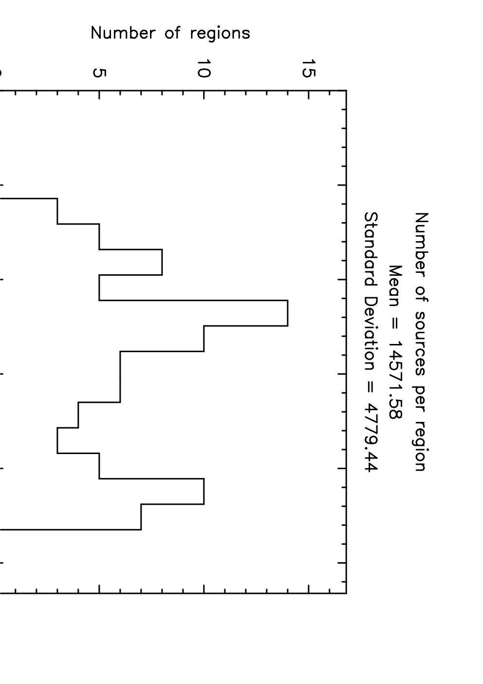
Sources were extracted from each of the IRIS2 images using the daophot tasks in the IRAF55 5 http://iraf.noao.edu/ package to produce a 2.14 m source catalogue (see Section 7.1 for more details). Examination of the residuals after removing the stellar flux from the image shows the stars have generally been well extracted despite different background levels across the image (caused by varying extended emission and extinction) and the crowded field. Figure 1 shows a histogram of the number of sources detected per region (which varied between 6,000 to 25,000, corresponding to stellar densities 60 250 stars/arcmin2) and the median source photometric fit uncertainty per region (0.06 mag).
 |
 |
2.3 Photometric Calibration
The photometry was calibrated using the 2MASS catalogue towards each
region (see Section 3.1). The extracted IRIS2 sources
(Section 2.2) were first matched with the 2MASS
catalogue as outlined in Section 2.4. The mean
offset between the two catalogues was then calculated by plotting the
difference between the 2MASS magnitude and IRIS2 instrumental
magnitude of the matched stars as a function of the measured IRIS2
instrumental magnitude over a suitable magnitude range (typically
12 to 14, to avoid both IRIS2 saturation and the poorer 2MASS
sensitivity). Figure 2 shows a histogram of the
offset between the IRIS2 instrumental magnitude and 2MASS magnitude
for each region. The range in values is due to the different airmass
of the IRIS2 observations. The uncertainty in IRIS2 absolute
photometry was estimated from the standard deviation between IRIS2 and
2MASS magnitudes over a reliable magnitude range (12th
to 14th magnitude) after this offset had been
applied. Figure 2 shows a histogram of the
estimated photometric accuracy towards each region, which is
0.13 magnitudes averaged over all the fields. This is
approximately twice the statistical error from the photometric fitting
(see Figure 1). Some of this scatter is likely
to be due to the difference between the MKO photometric system used by
IRIS2 and the 2MASS photometric
system66
6
http://www.astro.caltech.edu/jmc/
2mass/v3/transformations/
(Carpenter 2001). Of particular relevance to this work, the Ks
filters of the two photometric systems are responsive over different
wavelength ranges – from 1.982 to 2.306 m for IRIS2 and 1.915
to 2.384 m for 2MASS. Although converting to the 2MASS
photometric system may marginally reduce this scatter, the colour
correction terms are not characterised for sources with (J-H) 1.5,
(H-K) 1 and (J-K) 2. These are the reddest, most embedded
sources and thus likely to be of most interest to studies of star
formation.
 |
 |
 |
 |
 |
Figure 3 shows histograms of brightest, median and faintest magnitude of sources detected per region. Depending on the field, stars brighter than 11th magnitude in the IRIS2 fields suffer from saturation. Column 11 in Table 1 gives the minimum reliable magnitude for each region, corresponding to the maximum flux per field over which the array responded linearly. Photometry for stars brighter than this should be taken from the 2MASS catalogue.
Table 1 also provides information on the extracted IRIS2 2.14m source populations, image quality and photometric calibration towards each of the regions. The photometric data themselves are provided in an online catalogue in Table 2. We provide here the first five lines and a description of the PSC contents. These are further combined with the photometry for matched sources in the GLIMPSE catalogue (see Section 2.4). The first five lines of the combined catalogue are provided here, with the rest in the online material.
2.4 Matching sources at different wavelengths
Analysis of source colours relies on the ability to accurately match sources in the catalogues at different wavelengths. With too many sources (104) to check manually and crowded stellar fields, there is a potential problem of either matching a source multiple times or mismatching the sources completely. The resulting mismatched sources may replicate the large colour differences of embedded sources and hence contaminate the sample. To test the matching accuracy, we generated and matched synthetic catalogues with known offsets from a list of absolute source positions. In order to ensure a realistic spatial distribution of sources, including over densities due to clustering and under densities due to extinction, the absolute coordinates were taken from the 2MASS PSC of the region. The coordinates recorded in the synthetic catalogues were randomly offset from the absolute values by a 2D Gaussian distribution. Several synthetic catalogues were produced using the known absolute pointing error of the relevant datasets to generate the positional offsets. The sources in the synthetic catalogues were given a unique ID and then matched in the same way as the observed datasets using the tmatch routine in the tables.ttools package in IRAF. The routine matches every source in the first catalogue with the nearest counterpart in the second catalogue within a user defined matching radius. Comparing the ID of the matched sources in the synthetic catalogues it is possible to unambiguously identify which sources have been matched correctly.
The IRIS2 images were all individually registered with 2MASS images so have a relative astrometric uncertainty of (0.1 pixel) [see Section 2.1]. The astrometric uncertainty in the 2MASS and GLIMPSE surveys are both quoted as 0.3′′. However, the GLIMPSE survey coordinates were also registered with 2MASS data so the relative uncertainty between the IRIS2 and GLIMPSE catalogues should be considerably less than the assumed error of . Matching two synthetic catalogues generated with an uncertainty of , an equal number of sources and a search radius of 2 pixels, produces a 100% recovery with no confusion due to doubles or mismatches. Matching catalogues generated with an uncertainty of but different numbers of sources also recovers 100% of the sources correctly but includes 0.05% double sources. With different numbers of sources in each catalogue, the matching order then becomes important. For example, matching the catalogue with larger to smaller numbers of sources may produce ‘multiple matches’, where several sources in the larger catalogue are within the matching radius of a source in the smaller catalogue. However, the number of correctly matched sources is the same, irrespective of the matching order. Varying the matching radius has little effect as long as it is significantly larger than the combined astrometric uncertainty.
Based on the above analysis, when matching the IRIS2 PSC with the GLIMPSE PSC and a matching radius of 1.2′′, we expect to recover at least 99.8% of the sources correctly with a maximum of 0.1% doubles and 0.12% mismatches. We therefore conclude that mismatches should not seriously affect the combined IRIS2/GLIMPSE PSCs.
3 Other Catalogue Data
3.1 2MASS - 2 micron All Sky Survey
Using two 1.3m telescopes in Arizona and Chile, the 2MASS survey scanned the entire sky at the J, H and Ks bands (1.25, 1.65 and 2.17m) (Skrutskie et al. 2006). The survey has a 10 limiting magnitude of 15.8, 15.1, 14.3 0.03 mag at J, H and Ks respectively with a pixel size of 2.0′′ and 0.1′′ pointing accuracy. We make use of this data to provide a reference frame for the images as well as to provide the flux calibration.
3.2 GLIMPSE - Galactic Legacy Infrared Mid-Plane Survey Extraordinaire
Using the infrared array camera (IRAC) on-board the Spitzer Space Telescope (SST77 7 http://ssc.spitzer.caltech.edu/), the GLIMPSE survey has observed the galaxy at 3.6, 4.5, 5.8 and 8.0m with a 1.2” pixel size between and (Benjamin et al. 2003). The photometric accuracy is 0.2 and 0.3 mag for bands 1/2 and 3/4 respectively. The astrometric accuracy of the point source catalogue is 0.3′′. We combine this with the AAT data to construct a source catalogue from 2.14 to 8.0m.
4 The data
Figures 7 to 92 show the IRIS2 2.14 m images towards each of the regions overlayed with the methanol maser emission from Walsh et al. (1998). Note that in most cases, regions of extinction are readily apparent. Rarely is there a 2m point source associated with a methanol maser. In many cases, extensive regions of 2m nebulosity are seen. Several targetted regions overlap within a few arcminutes (e.g. G14.99-0.70 and G15.03-0.68 in the vicinity of M17) but each field was imaged independently to ensure uniform coverage (within the observational systematics) in the 5.7 inner region of the mosaic with optimum sensitivity (see Section 2).
Table 2 shows an example extract from the first five lines of the IRIS2 Ks-band (2.14 m) point source catalogue for a sample region. Sections 4.1 & 4.2 examine the issues of seeing and completeness in these Ks-band (2.14 m) PSCs including photometry for these sources.
The fits images, IRIS2 PSCs and IRIS2/GLIMPSE PSCs for each region are available through the Centre de Données astronomiques de Strasbourg (CDS)88 8 http://cds.u-strasbg.fr/. Photometric calibration for the fits images is provided by the fits header keyword, ‘‘MAGZERO’’, which gives the magnitude in each image corresponding to a flux count of 199 9 i.e. m = mZP - 2.5 log(f), where f is the number of counts determined for a source of interest in the fits images. This is the same value as that given in column 6 of Table 1.
4.1 Seeing
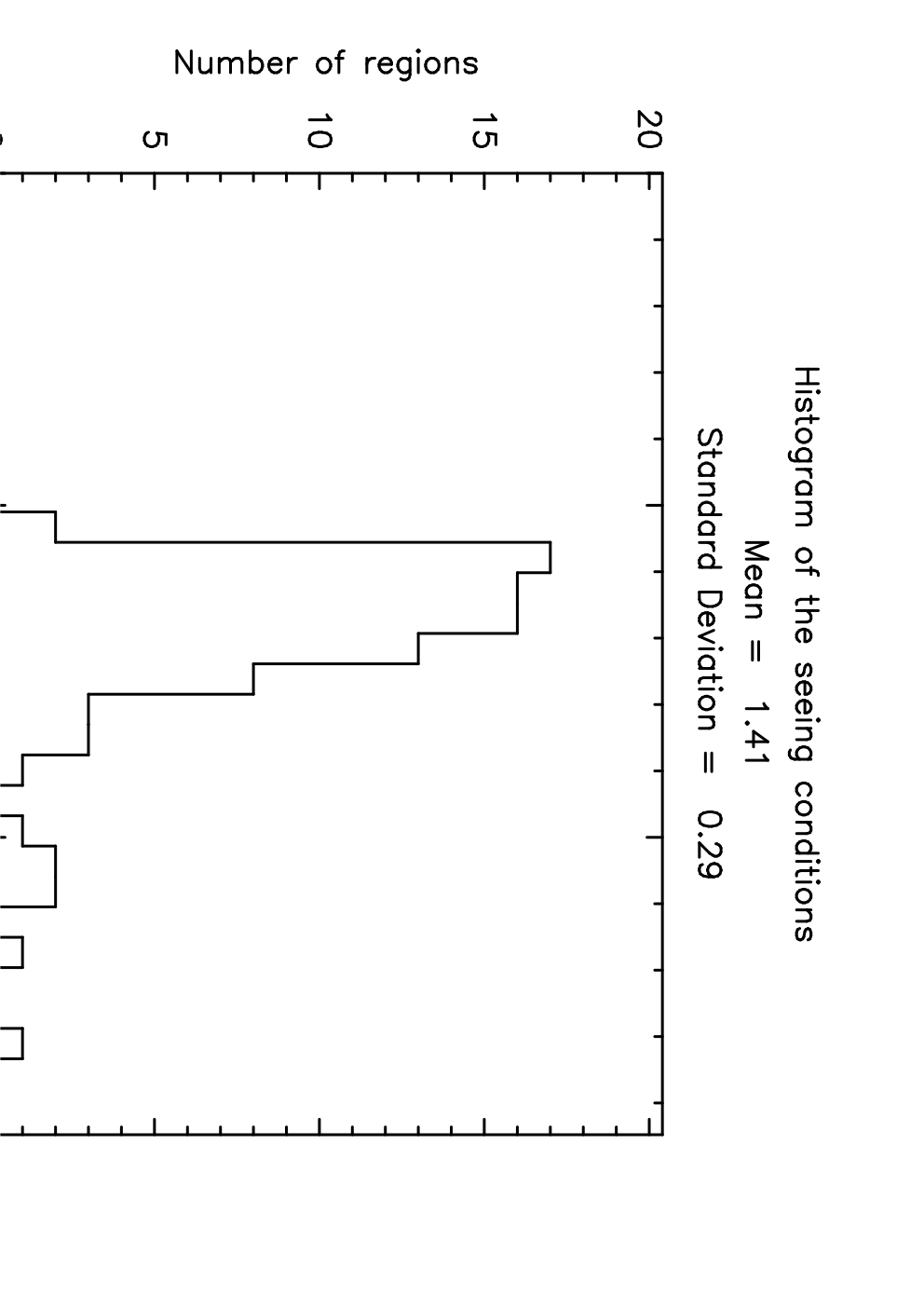
Figure 4 shows a histogram of the seeing conditions during observations of each of the regions. The majority of regions were observed in seeing of 1.2 to 1.4 arcseconds, a noticeable improvement on the 2′′ resolution of both 2MASS and GLIMPSE. The other two plots in Figure 4 show the effects of seeing on the brightest magnitude and number of sources detected. When the seeing is poor, the flux from bright stars is spread over more pixels and brighter stars can be recovered. Given the crowded nature of the observed fields towards the Galactic plane, it is unsurprising that the number of sources detected increases dramatically as the seeing decreases. The inverse linear relation between source counts and seeing suggests the difference in source counts resulting mostly due to the seeing present at the time of each observation.
 |
 |
 |
4.2 Completeness
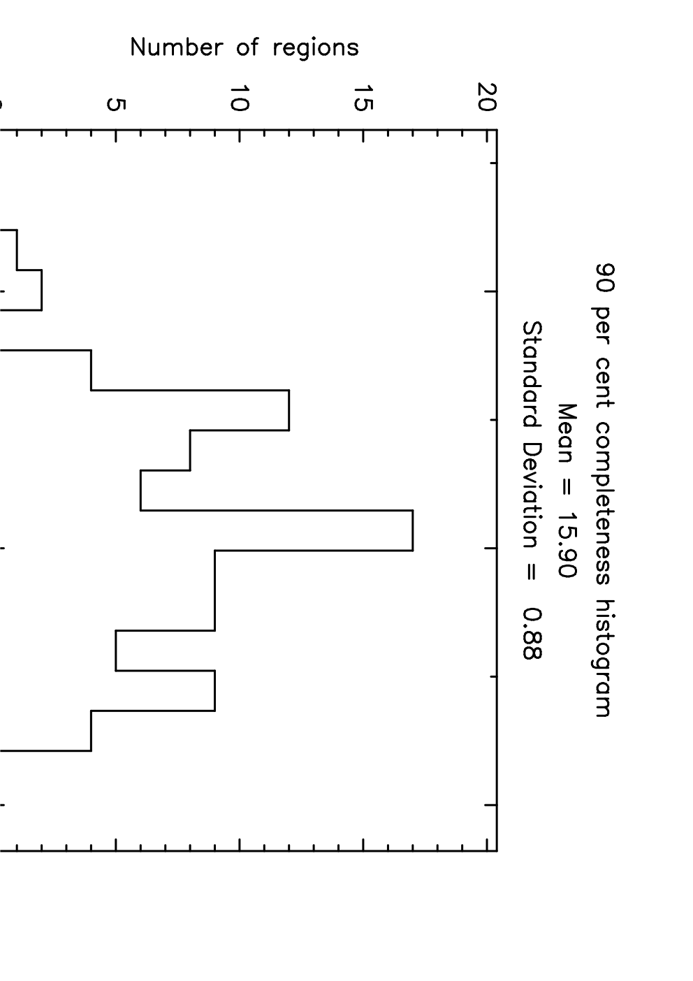
Longmore et al. (2007, hereafter L07B) used artificial star recovery to investigate the spatial variation in point source sensitivity as a function of wavelength for the field associated with G305.2+0.2. Having calculated the PSF for each image, a grid of artificial stars of the same magnitude separated by 30′′ was placed across the image. The same automated finding technique outlined in Section 2 was then used to calculate how many of the artificial stars were recovered. By shifting the 3030′′ grid of artificial stars in small steps through the image, it was possible to measure the completeness at 5′′ intervals without the PSF of individual artificial stars overlapping. The process was repeated by increasing the artificial star magnitudes in steps of 0.5 mag until no more stars were recovered. By recording the largest recovered magnitude at each position and wavelength it was possible to build a three-dimensional picture of the point source sensitivity across the region. The relative completeness as a function of position was then calculated at each wavelength by subtracting the median completeness magnitude at that wavelength from every position. This method is similar to that used by Gutermuth (2005) in an analysis of completeness limits of Spitzer IRAC data. Through analysis of the results from the artificial star recovery method, L07B found a simpler, empirical method of estimating the 90% completeness limit by calculating the turnover in the histogram of the number of stars as a function of magnitude which yields approximately the same limit as the full analysis. This metric is provided in Table 1, but we stress that a comprehensive analysis of each field would require this completeness limit to be determined individually for each. Figure 5 presents the histogram of this distribution of turnover magnitude.
5 Applications
As an example of what the data has the potential to provide once a full completeness analysis is conducted, we show the results towards G305.2+0.2, as reported by L07B. Figure 6 shows the slope of the spectral energy distribution between 2.14 and 4.5 m (i.e. ) of all sources detected towards i) a control field using a combined 2MASS/GLIMPSE PSC, ii) the target field using a combined 2MASS/GLIMPSE PSC and iii) the target field using a combined IRIS2/GLIMPSE PSC. The spectral index is related to the categories of young stellar objects (Class I, II, III), with younger sources tending towards larger spectral indexes. In this way the PSC provides a measure of the distribution of evolutionary states of the embedded cluster seen towards G305.2+0.2. The considerably more sensitive 2.14 m IRIS2 images means much more deeply embedded (redder) sources are detected with the IRIS2/GLIMPSE PSC compared to the 2MASS/GLIMPSE PSC. This is obvious in the bottom panel of Figure 6 as a significant increase in the number of sources with compared to the middle panel.

6 Acknowledgements
We thank Stuart Ryder for help with the data reduction. SNL was partially funded by an internal grant from UNSW.
References
- Benjamin et al. (2003) Benjamin R. A., Churchwell E., Babler B. L., Bania T. M., Clemens D. P., Cohen M., Dickey J. M., Indebetouw R., Jackson J. M., Kobulnicky H. A., +10 authors 2003, PASP, 115, 953
- Carpenter (2001) Carpenter J. M., 2001, AJ, 121, 2851
- Gutermuth (2005) Gutermuth R. A., 2005, PhD thesis, University of Rochester, United States – New York
- Longmore et al. (2007) Longmore S. N., Burton M. G., Barnes P. J., Wong T., Purcell C. R., Ott J., 2007, MNRAS, 379, 535
- Longmore et al. (2006) Longmore S. N., Burton M. G., Minier V., Walsh A. J., 2006, MNRAS, 369, 1196
- Longmore et al. (2007) Longmore S. N., Maercker M., Ramstedt S., Burton M. G., 2007, MNRAS, 380, 1497
- Purcell et al. (2006) Purcell C. R., Balasubramanyam R., Burton M. G., Walsh A. J., Minier V., Hunt-Cunningham M. R., Kedziora-Chudczer L. L., Longmore S. N., and 26 other authors 2006, MNRAS, 367, 553
- Purcell et al. (2009) Purcell C. R., Longmore S. N., Burton M. G., Walsh A. J., Minier V., Cunningham M. R., Balasubramanyam R., 2009, MNRAS, 394, 323
- Skrutskie et al. (2006) Skrutskie M. F., Cutri R. M., Stiening R., Weinberg M. D., Schneider S., Carpenter J. M., Beichman C., Capps R. e., 2006, AJ, 131, 1163
- Walsh et al. (1998) Walsh A. J., Burton M. G., Hyland A. R., Robinson G., 1998, MNRAS, 301, 640
- Walsh et al. (1997) Walsh A. J., Hyland A. R., Robinson G., Burton M. G., 1997, MNRAS, 291, 261
7 Appendix
Table 1 shows the properties of the IRIS2 2.14 m PSCs for all the observed regions. Tables 2 & 3 show the first five lines of a sample IRIS2 2.14 m PSC and a sample combined IRIS2/GLIMPSE PSC, respectively, with the full tables available on line. Finally, Section 7.1 describes in detail how the DAOPHOT package (digi.daophot) in IRAF was used to automatically find and perform photometry on stars within the IRIS2 fields and hence create the point source catalogues.
| Region | IRASa | RA | Dec | Magnitudes | Num | FWHM | |||||||
|---|---|---|---|---|---|---|---|---|---|---|---|---|---|
| (J2000) | (J2000) | ZP | Min. | Med. | Max. | Minrel | 90% | sources | (arcsec) | ||||
| G290.40-2.91 | 10555-6242 | 10:57:34.0 | -62:59:3.6 | 0.11 | 22.95 | 8.1 | 17.0 | 18.6 | 0.16 | 11.0 | 17.5 | 8395 | 1.60 |
| G293.82-0.74 | 11297-6156 | 11:32:05.4 | -62:12:25.0 | 0.16 | 23.66 | 9.3 | 16.4 | 17.8 | 0.19 | 10.0 | 16.9 | 9380 | 1.21 |
| G305.20+0.21b | 13079-6218 | 13:11:10.5 | -62:34:38.9 | 0.20 | 24.01 | 5.3 | 16.1 | 18.5 | 0.06 | 11.0 | 17.5 | 11226 | 1.20 |
| G309.92+0.48 | 13471-6120 | 13:50:41.8 | -61:35:10.1 | 0.09 | 24.01 | 9.7 | 16.3 | 18.5 | 0.09 | 11.0 | 16.9 | 9689 | 1.47 |
| G312.11+0.26 | 14050-6056 | 14:08:49.3 | -61:13:26.0 | 0.09 | 24.12 | 9.6 | 16.6 | 19.0 | 0.09 | 11.0 | 17.3 | 15439 | 1.66 |
| G313.77-0.86 | 14212-6131 | 14:25:01.6 | -61:44:58.1 | 0.08 | 24.20 | 9.5 | 15.9 | 18.5 | 0.06 | 11.0 | 16.9 | 11775 | 1.48 |
| G316.81-0.06 | 14416-5937 | 14:45:26.9 | -59:49:16.3 | 0.16 | 24.24 | 8.7 | 16.3 | 18.7 | 0.08 | 11.0 | 16.9 | 14796 | 1.24 |
| G318.95-0.20 | 14567-5846 | 15:00:55.3 | -58:58:53.6 | 0.22 | 24.11 | 9.5 | 16.5 | 18.8 | 0.09 | 12.0 | 17.1 | 20259 | 1.16 |
| G320.23-0.28 | 15061-5814a | 15:09:52.0 | -58:25:38.1 | 0.07 | 24.11 | 9.3 | 16.3 | 18.8 | 0.08 | 11.0 | 16.5 | 19299 | 1.40 |
| G321.03-0.48 | 15122-5801 | 15:15:51.6 | -58:11:17.4 | 0.14 | 24.09 | 9.7 | 15.3 | 17.8 | 0.04 | 11.0 | 15.6 | 10195 | 1.53 |
| G323.74-0.26 | 15278-5620 | 15:31:45.8 | -56:30:49.9 | 0.13 | 24.19 | 8.8 | 16.6 | 18.9 | 0.09 | 11.0 | 17.0 | 20356 | 1.19 |
| G327.12+0.51 | 15437-5343 | 15:47:32.7 | -53:52:38.5 | 0.10 | 24.15 | 9.5 | 15.7 | 18.1 | 0.05 | 11.0 | 16.0 | 11281 | 1.50 |
| G327.40+0.44 | 15454-5335 | 15:49:19.5 | -53:45:13.9 | 0.06 | 24.09 | 9.7 | 15.8 | 18.1 | 0.06 | 11.0 | 16.6 | 13947 | 1.36 |
| G331.28-0.19 | 16076-5134 | 16:11:26.9 | -51:41:56.6 | 0.14 | 24.19 | 9.6 | 16.2 | 18.6 | 0.07 | 11.0 | 17.0 | 17974 | 1.22 |
| G332.73-0.62 | 16158-5055 | 16:20:02.7 | -51:00:32.0 | 0.09 | 24.95 | 9.6 | 15.9 | 18.5 | 0.07 | 12.0 | 16.0 | 16424 | 1.24 |
| G337.71-0.05 | 16348-4654 | 16:38:29.6 | -47:00:35.7 | 0.11 | 23.93 | 7.9 | 14.6 | 17.7 | 0.04 | 10.0 | 15.0 | 10598 | 1.80 |
| G348.71-1.04 | 17167-3854 | 17:20:04.0 | -38:58:30.0 | 0.31 | 24.22 | 9.6 | 15.8 | 18.4 | 0.06 | 11.0 | 16.0 | 13465 | 1.21 |
| G0.21+0.00 | 17430-2844 | 17:46:07.7 | -28:45:20.0 | 0.17 | 24.08 | 9.5 | 13.2 | 15.9 | 0.04 | 11.0 | 13.6 | 14013 | 1.33 |
| G0.26+0.01 | - | 17:46:11.4 | -28:42:48.0 | 0.15 | 24.07 | 9.6 | 13.6 | 16.6 | 0.04 | 11.0 | 14.1 | 17314 | 1.35 |
| G0.32-0.20 | 17439-2845 | 17:47:09.1 | -28:46:16.1 | 0.16 | 24.06 | 9.4 | 14.3 | 17.2 | 0.06 | 11.0 | 15.2 | 19494 | 1.30 |
| G0.50+0.19 | 17429-2823 | 17:46:04.0 | -28:24:51.3 | 0.13 | 24.11 | 9.2 | 14.0 | 16.6 | 0.05 | 11.0 | 14.8 | 20703 | 1.25 |
| G0.55-0.85 | 17470-2853 | 17:50:14.5 | -28:54:31.2 | 0.15 | 23.34 | 8.2 | 14.1 | 17.3 | 0.05 | 11.0 | 14.1 | 12628 | 1.50 |
| G0.70-0.04 | 17441-2822a | 17:47:24.7 | -28:21:43.7 | 0.10 | 24.13 | 9.2 | 14.5 | 17.1 | 0.05 | 11.2 | 14.9 | 17241 | 1.30 |
| G0.84+0.18 | 17436-2807 | 17:46:52.8 | -28:07:35.3 | 0.13 | 24.19 | 8.8 | 14.3 | 16.8 | 0.05 | 12.0 | 14.7 | 21439 | 1.23 |
| G1.15-0.12 | 17455-2800 | 17:48:48.5 | -28:01:11.8 | 0.16 | 24.22 | 9.0 | 14.9 | 17.6 | 0.05 | 12.0 | 15.2 | 19274 | 1.22 |
| G2.54+0.20 | 17480-2636 | 17:50:46.5 | -26:39:44.9 | 0.17 | 24.14 | 8.8 | 14.8 | 17.6 | 0.04 | 11.0 | 15.0 | 15821 | 1.27 |
| G5.90-0.43 | 17574-2403 | 18:00:40.9 | -24:04:20.6 | 0.18 | 24.20 | 8.8 | 15.7 | 18.3 | 0.06 | 11.5 | 16.2 | 18643 | 1.12 |
| G6.54-0.11 | 17577-2320a | 18:00:50.9 | -23:21:29.4 | 0.11 | 24.35 | 9.0 | 15.3 | 18.1 | 0.06 | 11.5 | 15.7 | 22674 | 1.10 |
| G6.61-0.08 | 17577-2320b | 18:00:54.1 | -23:17:02.0 | 0.13 | 24.28 | 8.9 | 15.3 | 18.0 | 0.06 | 11.5 | 15.5 | 21661 | 1.08 |
| G8.14+0.23 | 17599-2148 | 18:03:00.8 | -21:48:10.4 | 0.15 | 24.28 | 9.0 | 15.7 | 18.4 | 0.06 | 11.5 | 15.9 | 22195 | 1.11 |
| G8.67-0.36 | 18032-2137a | 18:06:19.0 | -21:37:31.9 | 0.13 | 23.35 | 7.9 | 15.1 | 17.7 | 0.06 | 11.0 | 15.8 | 9400 | 1.32 |
| G9.62+0.19 | 18032-2032 | 18:06:14.8 | -20:31:37.0 | 0.11 | 24.30 | 8.9 | 15.7 | 18.3 | 0.06 | 11.7 | 16.5 | 21904 | 1.16 |
| G9.99-0.03 | 18048-2019 | 18:07:50.1 | -20:18:56.7 | 0.12 | 24.30 | 9.0 | 15.6 | 18.3 | 0.06 | 11.5 | 16.5 | 21436 | 1.13 |
| G10.29-0.13 | 18060-2005d | 18:08:49.4 | -20:05:59.0 | 0.13 | 24.28 | 9.0 | 16.2 | 18.7 | 0.07 | 11.5 | 17.0 | 21420 | 1.11 |
| G10.30-0.15 | 18060-2005a | 18:08:55.6 | -20:05:58.0 | 0.19 | 24.29 | 9.1 | 16.2 | 18.8 | 0.07 | 12.0 | 17.0 | 21093 | 1.16 |
| G10.34-0.14 | 18060-2005b | 18:09:00.0 | -20:03:35.5 | 0.20 | 24.32 | 9.2 | 16.3 | 18.9 | 0.08 | 12.0 | 17.0 | 21122 | 1.13 |
| G10.47+0.03 | 18056-1952b | 18:08:38.2 | -19:51:49.7 | 0.13 | 24.30 | 8.7 | 15.9 | 18.7 | 0.07 | 11.5 | 16.8 | 22054 | 1.16 |
| G10.48+0.03 | 18056-1952a | 18:08:37.9 | -19:51:15.0 | 0.14 | 24.29 | 8.6 | 15.8 | 18.4 | 0.06 | 11.3 | 16.5 | 20601 | 1.17 |
| G10.63-0.33 | 18075-1956b | 18:10:18.0 | -19:54:04.6 | 0.10 | 24.24 | 9.3 | 16.6 | 19.0 | 0.08 | 11.5 | 17.2 | 20965 | 1.15 |
| G10.63-0.38 | 18075-1956a | 18:10:29.2 | -19:55:41.2 | 0.12 | 24.29 | 9.2 | 16.6 | 19.1 | 0.08 | 12.0 | 17.5 | 22555 | 1.13 |
| G11.50-1.49 | 18134-1942 | 18:16:22.1 | -19:41:27.5 | 0.10 | 24.30 | 8.8 | 16.7 | 19.0 | 0.10 | 11.5 | 17.2 | 22905 | 1.12 |
| G11.94-0.15 | 18094-1840 | 18:12:17.3 | -18:40:02.8 | 0.11 | 23.36 | 7.6 | 14.3 | 17.2 | 0.06 | 10.0 | 14.5 | 11676 | 1.37 |
| G11.94-0.62 | 18110-1854 | 18:14:00.9 | -18:53:26.6 | 0.23 | 24.08 | 9.3 | 15.4 | 18.2 | 0.05 | 11.5 | 16.0 | 15317 | 1.36 |
| G11.99-0.27 | 18099-1841 | 18:12:51.2 | -18:40:39.7 | 0.10 | 24.16 | 8.7 | 14.4 | 17.3 | 0.03 | 11.0 | 15.0 | 11967 | 1.60 |
| G12.03-0.03 | 18090-1832 | 18:12:01.9 | -18:31:55.7 | 0.16 | 24.15 | 8.2 | 14.3 | 17.2 | 0.04 | 11.0 | 14.9 | 12573 | 1.44 |
| G12.18-0.12 | 18097-1825Ab | 18:12:41.0 | -18:26:21.5 | 0.09 | 24.15 | 8.3 | 14.3 | 17.0 | 0.04 | 10.5 | 15.2 | 11727 | 1.47 |
| G12.21-0.09 | 18097-1825Aa | 18:12:37.5 | -18:24:08.0 | 0.10 | 24.12 | 9.5 | 14.5 | 17.0 | 0.04 | 11.0 | 15.0 | 13765 | 1.31 |
| G12.68-0.18 | 18117-1753a | 18:13:54.7 | -18:01:41.3 | 0.14 | 24.15 | 8.8 | 15.7 | 18.6 | 0.05 | 11.0 | 16.0 | 12419 | 1.45 |
| G12.72-0.22 | 18112-1801 | 18:14:07.0 | -18:00:37.0 | 0.14 | 24.24 | 9.5 | 16.0 | 18.5 | 0.06 | 11.0 | 16.0 | 13400 | 1.24 |
| G12.89+0.49 | 18089-1732 | 18:11:51.4 | -17:31:30.2 | 0.09 | 24.23 | 9.4 | 16.4 | 18.9 | 0.08 | 11.0 | 17.1 | 17238 | 1.19 |
| G12.91-0.26 | 18117-1753b | 18:14:39.5 | -17:52:00.2 | 0.14 | 24.26 | 9.4 | 17.1 | 19.3 | 0.11 | 11.0 | 17.5 | 13986 | 1.27 |
| G14.60+0.02 | 18141-1615 | 18:17:01.1 | -16:14:38.7 | 0.12 | 23.47 | 8.4 | 15.1 | 17.7 | 0.05 | 10.5 | 16.0 | 14734 | 1.30 |
| G14.99-0.70 | - | 18:20:23.1 | -16:14:43.0 | 0.18 | 24.25 | 9.1 | 14.7 | 17.6 | 0.05 | 11.0 | 15.5 | 6338 | 1.44 |
| G15.03-0.68 | 18174-1612 | 18:20:24.8 | -16:11:35.4 | 0.47 | 24.30 | 9.5 | 14.7 | 17.6 | 0.05 | 12.0 | 15.5 | 7107 | 1.21 |
| G16.59-0.05 | 18182-1433 | 18:21:09.1 | -14:31:48.7 | 0.12 | 24.30 | 8.7 | 15.8 | 18.5 | 0.07 | 11.0 | 16.0 | 20984 | 1.18 |
| G16.86-2.16 | 18265-1517 | 18:29:24.4 | -15:16:04.1 | 0.09 | 23.92 | 8.2 | 15.8 | 18.1 | 0.07 | 10.0 | 16.2 | 11039 | 1.53 |
| G19.36-0.03 | 18236-1205 | 18:26:25.2 | -12:03:52.8 | 0.11 | 24.26 | 8.7 | 15.6 | 18.4 | 0.06 | 11.5 | 15.8 | 18355 | 1.19 |
| G19.61-0.13 | 18244-1155 | 18:27:16.4 | -11:53:38.4 | 0.09 | 24.28 | 8.6 | 15.5 | 18.3 | 0.06 | 11.5 | 15.8 | 22645 | 1.21 |
| G19.70-0.27 | 18248-1158 | 18:27:55.9 | -11:52:39.1 | 0.16 | 24.23 | 8.9 | 14.6 | 17.2 | 0.05 | 11.5 | 15.0 | 15609 | 1.25 |
| G21.88+0.01 | 18282-0951 | 18:31:01.7 | -09:49:01.4 | 0.10 | 23.90 | 8.0 | 14.5 | 17.1 | 0.04 | 10.0 | 14.5 | 12113 | 1.45 |
| G22.36+0.07 | 18290-0924 | 18:31:44.1 | -09:22:12.7 | 0.10 | 23.91 | 8.0 | 15.0 | 17.7 | 0.05 | 10.0 | 15.0 | 11319 | 1.43 |
| G23.26-0.24 | 18317-0845 | 18:34:31.8 | -08:42:46.8 | 0.12 | 23.88 | 8.1 | 15.6 | 18.1 | 0.07 | 10.0 | 16.2 | 12914 | 1.38 |
| G23.44-0.18 | 18319-0834 | 18:34:39.2 | -08:31:32.5 | 0.15 | 23.87 | 8.2 | 15.8 | 18.2 | 0.08 | 11.0 | 16.4 | 12988 | 1.32 |
| G23.71-0.20 | 18324-0820 | 18:35:12.4 | -08:17:39.6 | 0.13 | 23.87 | 8.0 | 15.1 | 17.7 | 0.06 | 10.5 | 15.9 | 11840 | 1.35 |
| G24.79+0.08 | 18335-0711a | 18:36:12.3 | -07:12:11.1 | 0.11 | 24.14 | 9.6 | 16.0 | 18.4 | 0.07 | 11.0 | 16.5 | 16342 | 1.35 |
| G24.85+0.09 | 18335-0711b | 18:36:18.4 | -07:08:52.1 | 0.12 | 23.85 | 7.9 | 15.3 | 17.7 | 0.06 | 11.0 | 15.9 | 10667 | 1.42 |
| G25.65+1.05 | 18316-0602 | 18:34:20.9 | -05:59:40.4 | 0.14 | 23.91 | 8.1 | 16.0 | 18.3 | 0.08 | 11.0 | 16.5 | 11660 | 1.42 |
| G25.71+0.04 | 18353-0628 | 18:38:03.1 | -06:24:14.7 | 0.12 | 23.85 | 8.2 | 15.0 | 17.5 | 0.05 | 11.0 | 15.7 | 13210 | 1.35 |
| G25.83-0.18 | 18361-0627 | 18:39:03.6 | -06:24:09.9 | 0.16 | 23.88 | 8.0 | 15.1 | 17.7 | 0.06 | 11.5 | 15.9 | 16948 | 1.27 |
| G28.15+0.00 | 18403-0417a | 18:42:42.2 | -04:15:31.9 | 0.12 | 23.83 | 6.5 | 14.3 | 17.8 | 0.03 | 10.0 | 14.9 | 6051 | 2.61 |
| G28.20-0.05 | 23.597-0417b | 18:42:58.1 | -04:13:56.0 | 0.10 | 23.60 | 8.1 | 15.4 | 17.6 | 0.07 | 10.0 | 15.9 | 12790 | 1.29 |
| G28.28-0.36 | 18416-0420b | 18:44:13.3 | -04:18:03.0 | 0.11 | 23.91 | 6.9 | 14.6 | 18.1 | 0.05 | 10.0 | 15.1 | 8818 | 2.35 |
| G28.83-0.25 | 18421-0348b | 18:44:51.1 | -03:45:48.2 | 0.11 | 23.92 | 6.5 | 14.7 | 17.9 | 0.04 | 10.0 | 15.0 | 8751 | 2.15 |
| G28.85-0.23 | 18421-0348a | 18:44:47.8 | -03:44:16.8 | 0.11 | 23.94 | 7.3 | 14.3 | 17.3 | 0.03 | 10.5 | 14.5 | 6794 | 2.16 |
| G29.87-0.04 | 18434-0242b | 18:46:00.0 | -02:44:58.1 | 0.10 | 23.87 | 6.6 | 14.7 | 17.7 | 0.03 | 11.5 | 14.9 | 7586 | 2.00 |
| G29.96-0.02 | 18434-0242c | 18:46:04.8 | -02:39:19.7 | 0.10 | 23.93 | 7.3 | 15.2 | 18.0 | 0.04 | 11.5 | 15.2 | 8356 | 2.05 |
| G29.98-0.04 | 18434-0242a | 18:46:12.1 | -02:38:58.1 | 0.14 | 23.88 | 7.3 | 15.1 | 18.0 | 0.04 | 12.0 | 15.1 | 8381 | 2.09 |
| G30.59-0.04 | 18443-0210 | 18:47:18.6 | -02:06:07.0 | 0.16 | 23.85 | 7.7 | 15.3 | 18.1 | 0.05 | 11.0 | 15.2 | 9618 | 1.74 |
| G30.71-0.06 | 18450-0200d | 18:47:36.5 | -02:00:31.3 | 0.16 | 23.87 | 7.8 | 15.4 | 18.0 | 0.05 | 11.0 | 15.2 | 9455 | 1.74 |
| G30.78+0.23 | 18440-0148c | 18:46:41.5 | -01:48:32.2 | 0.11 | 23.92 | 7.9 | 15.4 | 17.9 | 0.05 | 10.0 | 16.0 | 9226 | 1.56 |
| G30.79+0.20 | 18440-0148b | 18:46:48.1 | -01:48:46.0 | 0.11 | 23.93 | 8.1 | 15.9 | 18.4 | 0.07 | 10.0 | 16.5 | 12339 | 1.61 |
| G30.82-0.05 | 18450-0200a | 18:47:46.5 | -01:54:16.8 | 0.13 | 23.86 | 8.0 | 15.5 | 18.0 | 0.06 | 10.0 | 16.1 | 11487 | 1.43 |
| G30.82+0.28 | 18440-0148a | 18:46:36.1 | -01:45:18.2 | 0.20 | 23.91 | 8.2 | 15.5 | 17.9 | 0.05 | 10.0 | 16.1 | 11223 | 1.43 |
| G30.90+0.16 | 18446-0150 | 18:47:09.2 | -01:44:09.4 | 0.11 | 23.81 | 8.1 | 15.5 | 18.1 | 0.05 | 11.0 | 16.1 | 10363 | 1.47 |
| G31.06+0.09 | 18452-0141 | 18:47:41.2 | -01:37:21.3 | 0.12 | 23.83 | 8.1 | 15.6 | 18.1 | 0.06 | 11.0 | 16.2 | 14469 | 1.33 |
| G31.28+0.06 | 18456-0129 | 18:48:12.4 | -01:26:22.6 | 0.10 | 23.89 | 8.0 | 15.6 | 18.2 | 0.05 | 10.0 | 16.3 | 11903 | 1.55 |
| G31.41+0.31 | 18449-0115 | 18:47:34.3 | -01:12:47.1 | 0.10 | 23.93 | 8.2 | 15.4 | 17.9 | 0.05 | 11.0 | 16.2 | 12839 | 1.49 |
| R.A. | Dec. | Mag. | Mag. |
|---|---|---|---|
| 272.1961 | -20.1837 | 16.133 | 0.065 |
| 272.2225 | -20.1838 | 17.37 | 0.144 |
| 272.2219 | -20.1837 | 17.108 | 0.119 |
| 272.2214 | -20.1837 | 17.31 | 0.125 |
| 272.2209 | -20.1833 | 15.706 | 0.041 |
| ID | RA J2000 | Dec. J2000 | Ks | Ks | 3.6 | 3.6 | 4.5 | 4.5 | 5.8 | 5.8 | 8.0 | 8.0 |
|---|---|---|---|---|---|---|---|---|---|---|---|---|
| GLIMPSE | (degrees) | (degrees) | (mag) | (mag) | (mag) | (mag) | (mag) | (mag) | (mag) | (mag) | (mag) | (mag) |
| SSTGLMC_G010.2102-00.1517 | 272.1905 | -20.17984 | 12.86 | 0.02 | 11.90 | 0.10 | 11.72 | 0.09 | 11.79 | 0.25 | null | null |
| SSTGLMC_G010.2213-00.1721 | 272.2152 | -20.18006 | 14.02 | 0.02 | 11.86 | 0.07 | 11.43 | 0.07 | 10.10 | 0.13 | 10.83 | 0.01 |
| SSTGLMC_G010.2238-00.1767 | 272.2208 | -20.1801 | 12.02 | 0.04 | 11.51 | 0.08 | 11.54 | 0.09 | 11.35 | 0.15 | 10.53 | 0.16 |
| SSTGLMC_G010.2118-00.1511 | 272.1907 | -20.17816 | 13.25 | 0.02 | 12.04 | 0.08 | 12.11 | 0.13 | 11.71 | 0.19 | null | null |
| SSTGLMC_G010.2431-00.2087 | 272.2606 | -20.17873 | 14.06 | 0.02 | 12.42 | 0.08 | 12.06 | 0.10 | null | null | null | null |
7.1 Creating the point source catalogues
This section describes how the DAOPHOT package (digi.daophot) in IRAF was used to automatically find and perform photometry on stars within the IRIS2 fields and hence create the point source catalogues. Description of co-ordinate frame calibration, photometric calibration and catalogue matching are found in Section 2.
Set initial fitting parameters
As three seperate detector arrays were used over the course of the observations care was taken to measure the array specific input parameters (eg readout noise, gain, saturation value etc.) for each image. The image characteristics used by the star finding and photometry tasks were calculated using daoedit to pick out 10 bright, non-saturated, isolated stars with as little surrounding extended emission as possible. By fitting a radial profile to the emission, this task then calculates the FWHM, SKY (median) and for each of the stars. After calculating a sensible average value for each of these parameters from stars with good profiles, the values are then entered into several ‘pars’ tasks (which act as inputs into the finding/photometry tasks) as follows,
- •
epar datapars:
fwhmpsf = FWHM;
sigma = ;
datamin = SKY-(6);
datamax = “saturation value” (must be less than max value ie max ‘good’ data value); - •
epar centerpars:
cbox = 2FWHM or 5 (whichever is larger) - •
epar fitskypars:
salgori = mode (for crowded images);
annulus = 4xFWHM;
dannulus = 3.5FWHM - •
epar photpars:
aperture = 1FWHM - •
epar daopars:
psfrad = (4FWHM)+1;
fitrad = 1FWHM or 3 (whichever is larger)
Intial star list
After calculating the image parameters, the initial (first-pass) star list was created using the daofind task to run the search finding algorithm. This task was run several times using different detection thresholds between 3 and 5 and compared by eye to maximise finding fainter stars and excluding noise.
Initial photometry
Photometry of the stars in the first-pass list was calculated using daofind. Stars dumped by the task due to poor fits were manually checked to ensure no real stars were dropped. In practice, the dumped stars were either low signal noise spikes or saturated stars.
Calculating the point spread function
The task pstselect was used to select 10 bright, non-saturated, isolated stars across the image to calculate the PSF. A characteristic PSF for the image was then calculated from these PSF stars. The robustness of the PSF was checked by subtracting the characteristic PSF from the 10 selected stars and their nearest neighbours and inspecting the residuals. In an iterative process, bad PSF stars were removed and the procedure repeated until good residuals were seen across the image meaning a realiable characteristic PSF for that image had been obtained.
Extracting the stars and fitting world coords
Once the optimal image parameters and characteristic PSF had been obtained, the PSF model was fit to all the stars using allstar. The residuals after the PSF subtraction were carefully checked to ensure both bright and faint stars across the image had been successfully subtracted. The star coordinates were converted from pixels to world coordiates using wcsctran.