Directional variations of the non-Gaussianity parameter
Abstract
We investigate local variations of the primordial non-Gaussianity parameter in the WMAP data, looking for possible influence of foreground contamination in the full-sky estimate of . We first improve the needlet bispectrum estimate in ( Rudjord et al. 2009) on the full-sky to using the KQ75 mask on the co-added V+W channel. We find no particular values of estimates close to the galactic plane and conclude that foregrounds are unlikely to affect the estimate of in the V and W bands even for the smaller KQ85 mask. In the Q band however, we find unexpectedly high values of in local estimates close to the galactic mask, as well as significant discrepancies between Q band estimates and V/W band estimates. We therefore conclude that the Q band is too contaminated to be used for non-Gaussianity studies even with the larger KQ75 mask. We further noted that the local estimates on the V+W channel are positive on all equatorial bands from the north to the south pole. The probability for this to happen in a universe with is less than one percent.
Subject headings
cosmic microwave background — cosmology: observations — methods: statisticalI. Introduction
Although the Cosmic Microwave Background (CMB) fluctuations are usually assumed to follow a Gaussian distribution, the consensus is that this is only an approximation valid to a certain level of precision. The deviations from Gaussianity seem to be small and are therefore difficult to estimate precisely. However, accurate knowledge of both the size and nature of such a deviation would be of high value in cosmology. The search for such anomalies in the CMB has therefore attracted much attention recently.
Most models for inflation predict the CMB fluctuation to be slightly non-Gaussian. This level of non-Gaussianity is measured by the parameter (see e.g. [2]). Alternative inflationary scenarios predict different values of , thus making an accurate estimate of this parameter crucial for understanding the physics of the inflationary era. Several parameters have been considered in the literature, corresponding to different ansatz for the shape of primordial non-Gaussianities. In this paper we focus on local non-Gaussianity, parametrized by (simply in the following).
In [22], we used needlets to estimate a value of (local type) different from zero at the level. This was in agreement with previous estimates [26, 13, 23, 3, 4, 20, 21] where values of deviating from zero with about were also reported. Also in agreement with previous estimates, we found that the value of increases with smaller sky cuts. This could be a result of smaller error bars due to the increased amount of data, or it could be an indication of foreground residuals near the galactic plane influencing the value of . This is our main motivation for estimating on smaller parts of the sky. By having local estimates of we can check whether the high value of comes from areas close to the galactic plane thus indicating the influence of foreground residuals, or whether consistent values are found in different parts of the sky. The second motivation for studying the directional dependence of , is due to several reports of the CMB deviating from statistical isotropy in various ways [11, 9, 12, 6, 10, 25, 24]. Here we check whether a similar asymmetry is seen in the value of .
In [22], the bispectrum of spherical needlets [14] was used to obtain . The localization and uncorrelation properties of needlets make them a convenient tool for studying localized regions on the sky (see [1]). We will here use a similar analysis to estimate the level of non-Gaussianity on selected regions on the sky and in this way study the spatial variations of . We therefore refer the reader to ([22]) for a more detailed description of the procedure, as well as for a more extensive list of references.
This paper is organized as follows. In section II we describe the data used for the analysis, in section III we describe the non-Gaussian maps and in section IV we outline the method used for estimating . We apply the procedure to WMAP data and present the results in section V before we summarize and conclude in section VI.
II. Data
This analysis was performed using the foreground reduced co-added V+W frequency bands of the WMAP five year data at Healpix11 1 http://healpix.jpl.nasa.gov resolution . Also the individual Q, V and W bands were used for consistency tests. The Gaussian simulations were generated using the best fit power spectrum from the WMAP five year release. We also used the beam and noise properties supplied by the WMAP team. For masking out galactic foregrounds we used the KQ75 as well as the smaller KQ85 mask.
III. Non-Gaussian maps
The non-Gaussian maps used for the analysis have been generated using the algorithm developed in [15, 16] (see also [5] for recent developments). We briefly review the general structure of the algorithm here, while addressing the reader to the above mentioned papers for further details. The CMB multipoles are related to the primordial gravitational potential through the well known formula:
| (1) |
where is the radiation transfer function and the potential is written in Fourier space. However, for the case of primordial non-Gaussianity, the primordial potential takes a very simple expression in real space, where:
| (2) |
In the previous expression is a Gaussian random field, characterized by a primordial power spectrum ; in the following we will refer to as the Gaussian part of the primordial potential. The remaining non-Gaussian part of the potential is simply the square of the Gaussian part in each point (modulo a constant term, necessary to enforce the condition ; however it is clear that this term affects only the CMB monopole)
It is then convenient to work directly in real space and recast formula (1) in the following form
| (3) |
where are the real space transfer functions, is a spherical Bessel function, and is a lookback conformal distance. This formula suggests to structure the algorithm in the following steps
- 1.
Generate the Gaussian part of the potential in a box whose side is the present cosmic horizon.
- 2.
Square the Gaussian part point by point to get the non-Gaussian part.
- 3.
Expanding in spherical harmonics the Gaussian and non-Gaussian parts of the potential for different values of the radial coordinate in the simulation box.
- 4.
Convolve the spherical harmonic expansions of and with the radiation transfer function in order to obtain the Gaussian and non-Gaussian part of the multipoles of the final NG CMB simulation. For a given choice of the non-Gaussian parameter a CMB map is then obtained simply through the linear combination (the superscripts L and NL always indicating Gaussian and non-Gaussian respectively).
The most difficult and time consuming part in this process is actually the generation of the Gaussian part of the potential . The difficulty arise from the fact that we are working in a box of the size of the present cosmic horizon, that in conformal time is about Gpc, but at the same time a cell in this box must have a size no bigger than Mpc in order to resolve the last scattering surface, where most of the CMB signal is generated. It turns out (see [15, 16] for details and more explanations) that a convenient way to achieve this is to work directly in spherical coordinates, use a non uniform discretization of the simulation box (since no points are needed in a large region of the box where photons are just free streaming) and generate the multipoles of the expansion of through the following two step approach:
- 1.
Generate uncorrelated radial multipoles , gaussianly distributed and characterized by the following spectrum:
(4) where is the Dirac delta function.
- 2.
Filter the multipoles with suitable functions in order to produce a Gaussian random field with the properties of the multipole expansion of the primordial Gaussian potential . It can be shown that the expression of the filter functions is:
(5) where is the primordial power spectrum, and the filtering operation takes the form
(6) In the last expression are the desired quantities i.e. the multipoles of the expansion of the Gaussian part of the primordial potential for a given .
IV. Method
The bispectrum has shown to be the most powerful tool for estimating . The bispectrum is zero for a Gaussian field, and any significant deviations from a zero bispectrum is therefore a non-Gaussian signal. Needlets are a new type of spherical wavelets which were introduced by [18]. For our analysis we use the bispectrum of needlet coefficients [14] to estimate . The localization properties of needlets make it possible to obtain the bispectrum in several different regions of the sky with very little additional costs in terms of CPU time compared to one full sky analysis. Although the needlet bispectrum does not yield optimal error bars on (see [23] for the optimal method), the advantage is the possibility of a fast and easy calculation of local estimates for consistency checks.
The needlet coefficients are denoted , is frequency, the direction on the sky (we will take as the pixel number in the Healpix grid) and the parameter characterizes the localization in frequency domain. Indeed, needlets allow for a tight control of localization in harmonic space and uncorrelation in pixel space; these properties are valuable for statistical inference and are not shared by other wavelet constructions, please refer to [1]), [17] for details and further references (see also [19] and [7]). For instance, for a given value of a needlet coefficient only contains information on multipoles in the range . Thus, the parameter controls localization in harmonic space: small values of correspond to small ranges of frequencies , while the reverse is true for larger .
The needlet bispectrum with base may be expressed as
| (7) |
where are the standard deviation of the needlet coefficients for a Gaussian map and is the region of the sky for which the bispectrum is calculated.
For the estimation of we used a similar procedure as in [22], but with a few small changes. We used a higher value for , resulting in fewer needlet scales. Intuitively one would expect this to give a poor result, since each needlet scale would cover a large interval in -space. However, a higher value for also gives better localization properties in pixel-space, thus minimizing the influence of the mask and thereby reducing the error bars. Additionally, this greatly reduces the computational cost of the analysis.
We will calculate the needlet bispectra using the needlet coefficients calculated on the pixels of a map. We will use all the pixels which are inside an pixel as our smallest region . We thus obtain 48 bispectra where denotes a pixel of the pixelization. Having obtained these 48 bispectra it is straightforward to construct the bispectrum on sky patches with different shapes and sizes. We see from eq. 7 that the bispectrum of a larger patch is then simply
| (8) |
where the sum over goes over the pixels within the desired region.
In order to estimate we perform a analysis for every map and region to be investigated
| (9) |
where the data vector is
| (10) | |||||
is here the average first order non-Gaussian bispectrum obtained using non-Gaussian simulations [16]. See [22] for details. The corresponding covariance matrix is evaluated by means of Monte-Carlo simulations.
Differentiating to find the value for which gives the lowest yields the “Generalized Least Squares” estimate:
| (11) |
We estimate local values according to the procedure described in [22], but with one important difference: We calculate and save the bispectra calculated on each individual pixel for each simulation. Then, when the bispectrum and thereby is estimated for a larger region, the bispectra for the different pixels are added up according to eq. 8 and the correlation matrix is constructed from this final bispectrum for each larger region.
V. Results
First we estimated on the full sky using and needlet scales covering multipoles up to . This was the best trade-off (lowest error bars) between needlet coefficients for low values of being more affected by the mask but having more frequencies and for high values of being less affected by the mask but having fewer scales. Otherwise we followed the same procedure as in [22]. The results are presented in table 1.
| freq. channel | KQ75 | KQ85 |
|---|---|---|
| V + W | ||
| V | ||
| W | ||
| Q |
As we see from the results, the combined V + W channel gives a deviation from Gaussianity. The individual V and W channels are consistent (within ), but the Q channel deviates significantly from the others, suggesting possible contamination by foregrounds.
We repeat the above analysis on localized regions on the sphere. First the bispectra were found for an ensemble of Gaussian simulations on each of the Healpix patches on the sky. We then combined these patches in three different ways according to eq. 8.
- 1.
Hemispheres The larger regions were defined to be hemispheres. For each of the 48 directions defined by the pixel centers, was estimated on a hemisphere centered on this direction.
- 2.
discs Same as for the hemispheres, estimating on discs with radius instead of hemispheres.
- 3.
Equatorial rings These regions were defined to be the constant latitude rings in which the healpix pixels are ordered. Each of these rings covers a relatively small part of the sky, and the error-bars are therefore large. However they are not overlapping, and the estimates on the different rings can therefore be considered nearly independent (except for the largest scales).
The estimates from the discs with the smaller KQ85 mask are shown in figure 1, where each pixel represents the estimate on a disc centered on the pixel. The lower plot shows the same map, but for each region has been normalized by its standard deviation. We see that even for the smaller mask, there is no evidence for particularly high values of in the galactic region, but note that most of the values are positive. In figure 2 we show the corresponding map of estimates over hemispheres while using the KQ75 mask. As an additional test of consistency we have produced the same estimates based on bispectra obtained from pixels instead of pixels. The result is shown in the same figure. We can see that the two maps show the same structures on the sky.

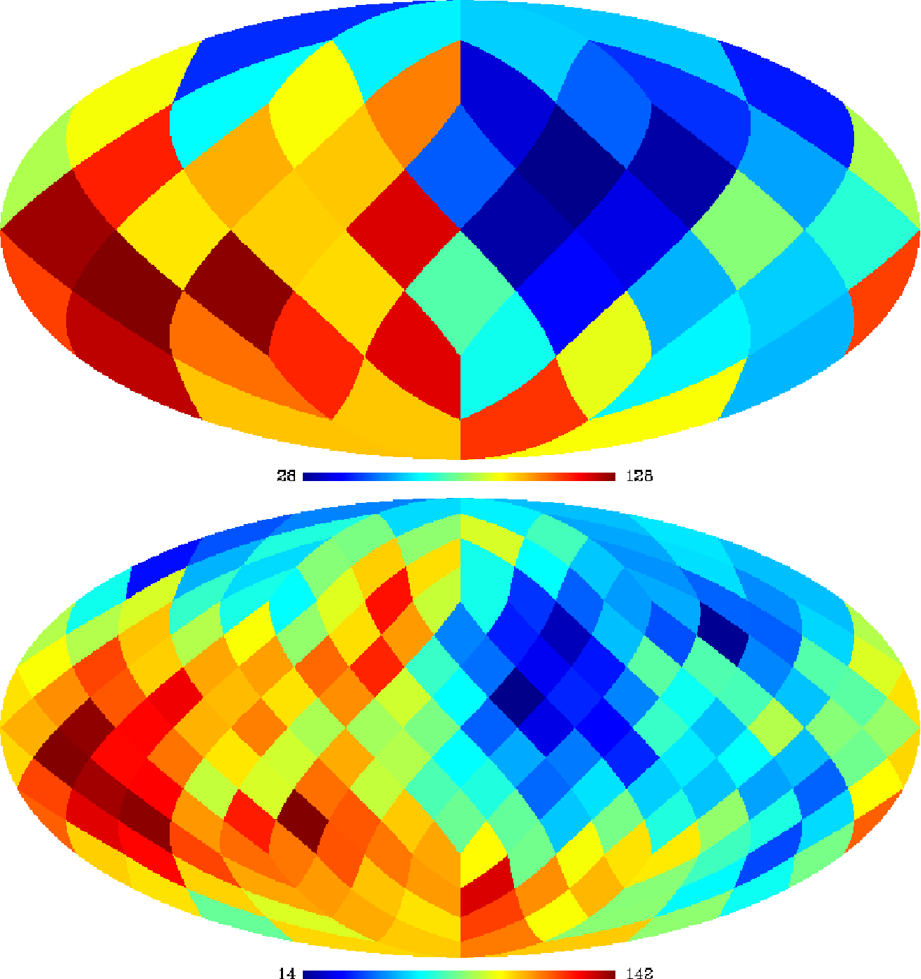
As seen from figure 1 the distribution of on the sky shows a dipole. For the map of the discs of the V+W channel (KQ85), the dipole has a maximum at , with an amplitude of . We investigated whether such a dipolar distribution of was common in Gaussian simulations and found the value of the dipole amplitude to be in good agreement with simulated maps. The dipole is therefore to be expected. Investigation of the hemisphere results as well as for the KQ75 mask using both the combined V+W channel and the individual Q, V and W frequency channels yielded similar results.
In order to check whether the 48 estimates of were internally consistent, we combined the estimates to form a data vector for a test. Simulations were then used to find a covariance matrix containing the covariances between the 48 estimates. Then a test was performed on Gaussian simulations as well as on the WMAP data. The values of the data were compared with those of the simulations. The results, both for the hemisphere estimates as well as for the disk estimates, was that the of the WMAP data was fully consistent with Gaussian simulations (within ). The local estimates are therefore internally consistent.
As a further test we obtained estimates of on equatorial rings. The motivation behind this approach was to uncover possible foreground contamination outside the KQ75 mask. The estimates for the different rings are presented in table 2. We see that the estimates of seem higher around equator, but the errors-bars are also larger (due to the galactic mask in the equatorial region). Since none of the rings show particularly high values (compared to the error bars) we do not have evidence to claim that foreground residuals have an influence of the estimates of . The internal consistency of the various ring estimates have been tested as described above and shown to be in agreement with simulations (within ).
We also estimated on the equatorial rings of the V + W map using the smaller KQ85 mask. These results are presented in table 2. As expected the error-bars are somewhat smaller then the results with the KQ75 mask, especially around the equatorial region. The estimates are consistent with the ones from the KQ75 mask.
We then followed through with similar investigations of the individual Q, V and W frequency channels using the KQ75 mask (table 2). The V and W channels are consistent (within ), while only the Q channel shows a deviation in the ring around equator exactly where foreground residuals would be expected. We thus suspect a possible influence of foreground contamination in this band. This was further checked by testing the consistency of the estimated between the bands using a approach. Whereas the (V-W) and (V-Q) differences were found to be consistent with simulations (within ), the (W-Q) difference was found to be larger than in of the simulations.
Also, a similar test was performed on the differences and . We see in table 1 and on some rings in table 2 that the VW estimates seem driven by the W estimate. This is not seen in simulated maps and it was found that the small difference found for the WMAP data is found in only of the simualted maps whereas the difference for WMAP was found to be consistent (well within ) with simulations.
| V+W | V+W | Q | V | W | |
|---|---|---|---|---|---|
| ring | KQ75 | KQ85 | KQ75 | KQ75 | KQ75 |
We see that all of the rings for the V+W channel (as well as the individual V and W channels) give a estimate . These rings are nearly independent (except for the largest scales) and for a sky with one would expect that each of these have a probability of being positive. For rings one would then expect only a probability that all rings give (this probability is confirmed by simulations).
Since the lowest value estimated for the rings of the V + W channel (with the KQ75 mask) is , we investigated the probability of this occurring in Gaussian simulations. We found that of Gaussian simulations, only have in all the rings.
VI. Conclusions
In this paper we have used the bispectrum of needlets to obtain local estimates of on the WMAP five year data. We performed the analysis on the combined V+W channel, as well as the individual Q, V and W channels, using multipoles up to and the KQ75 galactic cut. For the combined V+W channel we also applied the KQ85 mask.
We first made a full sky analysis, resulting in a best fit value of for the combined V+W channel using the KQ75 mask. The individual V and W channels give consistent (within ) results, but the estimate of the Q channel deviates significantly, suggesting contamination of foregrounds.
The estimates were then made on selected regions of the sky and showed how the needlet bispectrum approach is powerful for finding estimates of in many different regions, roughly at the cost of one single full sky estimate. We divided the sky into smaller regions according to four different patterns: hemispheres, disks and equatorial rings. In each of these schemes was estimated in every region. The results were compared to simulations using a test, and all local estimates were found to be internally consistent (within ) for the V and W channels.
The local estimates of showed a dipolar distribution of on the sphere, with a maximum at , . For comparison, the hemispherical power asymmetry reported in [11] was found with a maximum in , , and is therefore not expected to be connected to the findings in this paper.
Also, such a dipolar distribution was found to be common in simulated Gaussian maps. For the equatorial rings we found a positive value for in every ring. We compared the lower estimate of the V+W channel ( for all rings) with simulations and found that only of Gaussian simulations have this feature.
For the rings we find no significant evidence of foreground contamination outside the galactic KQ75 mask. The results also seem to be fairly consistent (within ) between the individual V and W channels whereas the Q band show signs of possible foreground contamination in the equatorial band where is larger than zero at the level. This is confirmed by the fact that the differences in local values between the Q and W bands are larger than in of the simulations.
We conclude that our study shows no significant anisotropy in the estimates of in the CMB sky. No abnormal values for are found close to the equator except for the Q band where we suspect foregrounds to influence the estimate of .
References
- [1] Baldi, P., Kerkyacharian, G., Marinucci, D. & Picard D. 2009, Annals of Statistics, Vol. 37, arXiv:math/0606599
- [2] Bartolo, N., Komatsu, E., Matarrese, S. & Riotto, A. 2004, Phys. Rept., 402, 103
- [3] Curto, A. et al., 2008, arXiv:0807.0231
- [4] Curto, A., Martinez-Gonzalez, E. & Barreiro, B. 2009, arXiv:0902.1523
- [5] Elsner, F. & Wandelt, B. D., 2009, ApJS 184 264
- [6] Eriksen, H. K., Hansen, F. K., Banday, A. J., Górski, K. M. & Lilje, P. B. 2004, ApJ, 605, 14
- [7] Fay, G., Guilloux, F., Betoule, M., Cardoso, J.-F. Delabrouille, J., Le Jeune, M. 2008, Phys.Rev. D78:083013, arXiv:0807.1113
- [8] Górski, K.M. et al. 2005, ApJ, 622, 759-771
- [9] Groeneboom, N. E. & Eriksen, H. K. 2009, ApJ, 690, 1807
- [10] Hansen, F. K., Banday, A. J. & Górski, K. M. 2004, MNRAS, 354, 641
- [11] Hansen, F. K., Banday, A. J., Górski, K. M., Eriksen, H. K. & Lilje, P. B. 2008, arXiv:0812.3795
- [12] Hoftuft, J. et al. 2009, in press, arXiv:0903.1229
- [13] Komatsu, E. et al. 2009, ApJS, 180, 330
- [14] Lan, X. & Marinucci, D., Electronic Journal of Statistics 2008, Vol. 2, 332-367, arXiv:0802.4020
- [15] Liguori, M., Matarrese S. and Moscardini, L., 2003, ApJ, 597, 57
- [16] Liguori, M. et al. 2007, Phys. Rev. D, 76, 105016
- [17] Marinucci, D. et al. 2008, MNRAS, 383, 539
- [18] Narcowich, F.J., Petrushev, P. & Ward, J.D. 2006, SIAM Journal of Mathematical Analysis 38, 2, 574
- [19] Pietrobon, D., Balbi, A., Marinucci, D. 2006, Physical Review D, 74, 043524
- [20] Pietrobon, D., Cabella, P., Balbi, A., de Gasperis, G. & Vittorio, N. 2008, arXiv:0812.2478
- [21] Pietrobon, D. et al. 2009, arXiv:0905.3702
- [22] Rudjord, O. et al 2009, arXiv:0901.3154
- [23] Smith, K. M., Senatore, L. & Zaldarriaga, M. 2009, arXiv:0901.2572
- [24] Tegmark, M., de Oliveira-Costa, A. & Hamilton, A. J. 2003, Phys. Rev. D, 68, 123523
- [25] Vielva, P., Martinez-Gonzalez, E., Barreiro, R. B., Sanz, J. L. & Cayon, L. 2004b, ApJ, 609, 22
- [26] Yadav, A. P. S. & Wandelt, B. D. 2008, Physical Review Letters, 100, 181301