Reduction Algorithm for the NPMLE for the Distribution Function
of Bivariate Interval Censored Data

Marloes H. Maathuis¹¹ 1 Marloes H. Maathuis is a Ph.D. student in the Department of Statistics, University of Washington, Seattle, WA 98195 (email: marloes@stat.washington.edu).
Department of Statistics, University of Washington, Seattle, WA 98195

Key words: Computational Geometry; Maximal Clique; Maximal Intersection; Parameter Reduction.

Abstract

We study computational aspects of the nonparametric maximum likelihood estimator (NPMLE) for the distribution function of bivariate interval censored data. The computation of the NPMLE consists of two steps: a parameter reduction step and an optimization step. In this paper we focus on the reduction step. We introduce two new reduction algorithms: the Tree algorithm and the HeightMap algorithm. The Tree algorithm is only mentioned briefly. The HeightMap algorithm is discussed in detail and also given in pseudo code. It is a very fast and simple algorithm of time complexity $O(n^{2})$ . This is an order faster than the best known algorithm thus far, the $O(n^{3})$ algorithm of Bogaerts and Lesaffre (2003). We compare our algorithms with the algorithms of Gentleman and Vandal (2001), Song (2001) and Bogaerts and Lesaffre (2003), using simulated data. We show that our algorithms, and especially the HeightMap algorithm, are significantly faster. Finally, we point out that the HeightMap algorithm can be easily generalized to $d$ -dimensional data with $d>2$ . Such a multivariate version of the HeightMap algorithm has time complexity $O(n^{d})$ .

1 INTRODUCTION

We consider the nonparametric maximum likelihood estimator (NPMLE) for the distribution function of bivariate interval censored data. Let $(X,Y)$ be the variables of interest and let $F_{0}$ be their joint distribution function. Suppose that there is a censoring mechanism, independent of $(X,Y)$ , so that $(X,Y)$ cannot be observed directly. Thus, instead of a realization $(x,y)$ , we observe a rectangular region $R\subset\mathbb{R}^{2}$ that is known to contain $(x,y)$ . We call $R$ an observation rectangle. Our data consists of $n$ i.i.d. observation rectangles $R_{1},\dots,R_{n}$ , and our goal is to compute the NPMLE $\hat{F}_{n}$ of $F_{0}$ .

Let $\mathcal{F}$ denote the class of all bivariate distribution functions. Furthermore, for each $F\in\mathcal{F}$ , let $P_{F}(R_{i})$ denote the probability that the pair of random variables $(X,Y)$ is in observation rectangle $R_{i}$ when $(X,Y)\sim F$ . Then, omitting the part that does not depend on $F$ , we can write the log likelihood as

\displaystyle l_{n}(F)=\sum_{i=1}^{n}\log(P_{F}(R_{i})),

(1)

and an NPMLE $\hat{F}_{n}\in\mathcal{F}$ is defined by

\displaystyle l_{n}(\hat{F}_{n})=\max_{F\in\mathcal{F}}\hskip 2.84544ptl_{n}(F).

As stated here, this is an infinite dimensional optimization problem. However, the number of parameters can be reduced by generalizing the reasoning of ?) for univariate censored data. By doing this (see e.g. ?), ?), ?)) one can easily derive that:

•

The NPMLE can only assign mass to a finite number of disjoint rectangles. We denote these rectangles by $A_{1},\dots,A_{m}$ and call them maximal intersections, following ?).
•

The NPMLE is indifferent to the distribution of mass within the maximal intersections.

The second property implies that the NPMLE is non-unique, in the sense that we cannot determine the distribution of mass within the maximal intersections. ?) call this representational non-uniqueness. Hence, we can at best hope to determine the amount of mass assigned to each maximal intersection. Let $\alpha_{j}$ be the mass assigned to maximal intersection $A_{j}$ , and let $\alpha=(\alpha_{1},\dots,\alpha_{m})$ . Then $P_{F}(R_{i})$ in equation (1) is simply the sum of the probability masses of the maximal intersections that are subsets of $R_{i}$ :

\displaystyle P_{F}(R_{i})=P_{\alpha}(R_{i})=\sum_{j=1}^{m}\alpha_{j}1_{\{{A_{j}\subset R_{i}}\}}.

We can then express the log likelihood in terms of $\alpha$ :

\displaystyle l_{n}(\alpha)

\displaystyle=\sum_{i=1}^{n}\log(P_{\alpha}(R_{i}))=\sum_{i=1}^{n}\log\Bigl(\sum_{j=1}^{m}\alpha_{j}1_{\{{A_{j}\subset R_{i}}\}}\Bigr).

(2)

Let $\mathcal{K}=\left\{\alpha\in\mathbb{R}^{m}:\alpha_{j}\geq 0,j=1,\dots,m\right\}$ and $\mathcal{A}=\{\alpha\in\mathbb{R}^{m}:\mathbf{1}^{T}\alpha=1\}$ , where $\mathbf{1}$ is the all-one vector in $\mathbb{R}^{m}$ . Then an NPMLE $\hat{\alpha}\in\mathcal{K}\cap\mathcal{A}$ is defined by

\displaystyle l_{n}(\hat{\alpha})=\max_{\alpha\in\mathcal{K}\cap\mathcal{A}}l_{n}(\alpha).

(3)

This is an $m$ -dimensional convex constrained optimization problem that does not need to have a unique solution in $\alpha$ . This forms a second source of non-uniqueness in the NPMLE. ?) call this mixture non-uniqueness.

Asymptotic properties of the NPMLE for univariate interval censored data have been studied by ?). In contrast to the consistency problems of the NPMLE for bivariate right censored data, the NPMLE for bivariate interval censored data has been shown to be consistent (?)). This implies that the NPMLE can be used in practical applications to estimate the distribution function of bivariate interval censored data, for example to analyze data from AIDS clinical trials (see e.g. ?)).

From the discussion above, it follows that the computation of the NPMLE consists of two steps. First, in the reduction step, we need to find the maximal intersections $A_{1},\dots,A_{m}$ . This reduces the dimensionality of the problem. Then, in the optimization step, we need to solve the optimization problem defined in (3).

In this paper we focus on the reduction step. We distinguish between two types of reduction algorithms that reflect a trade-off between computation time and space:

•

type 1: The reduction algorithm computes the maximal intersections $A_{1},\dots,A_{m}$ .
•

type 2: The reduction algorithm computes the clique matrix, an $m\times n$ matrix $C$ with elements $C_{ji}=1_{\{{A_{j}\subset R_{i}}\}}$ .

For $n$ observation rectangles, the number of maximal intersections is $O(n^{2})$ . Hence, given the observation rectangles, one can compute the clique matrix from the maximal intersections and vice versa in $O(n^{3})$ time.

We need $O(n^{2})$ space to store the maximal intersections, while we need $O(n^{3})$ space to store the clique matrix. Thus, type 1 algorithms require an order of magnitude less space to store the output. On the other hand, the choice of reduction algorithm determines the amount of computational overhead in the optimization step, where the values of the indicator functions $1_{\{{A_{j}\subset R_{i}}\}}$ are needed repeatedly. Namely, using a type 1 algorithm requires repeated computation of these indicator functions, while such computations are avoided with a type 2 algorithm. Thus, if we use a type 1 reduction algorithm, the computational overhead in the optimization step is increased by a constant factor.

Finally, it should be noted that the clique matrix provides useful information about mixture uniqueness of the NPMLE. For example, properties of the clique matrix are used to derive sufficient conditions for mixture uniqueness by ?) and ?). We can also use the clique matrix to describe the equivalence class of solutions to (3). Let $\hat{\alpha}$ be a solution, and consider $\left(C^{T}\hat{\alpha}\right)_{i}=P_{\hat{\alpha}}(R_{i})$ , $i=1,\dots,n$ . Since the log likelihood (2) is strictly concave in $P_{\alpha}(R_{i})$ , the vector $C^{T}\hat{\alpha}$ is unique. Thus, the equivalence class of NPMLEs is exactly the set $\{\alpha\in\mathcal{K}\cap\mathcal{A}:C^{T}\alpha=C^{T}\hat{\alpha}\}$ , since all $\alpha$ ’s in this set yield the same likelihood value.

We now give a brief overview of existing reduction algorithms. ?) provide a simple, but not very efficient, type 1 algorithm. ?) introduce a type 2 algorithm of time complexity $O(n^{5})$ . ?) proposes a type 1 algorithm that is of comparable speed. The algorithm with the best time complexity so far is the $O(n^{3})$ type 1 algorithm of ?). Finally, ?) gives an $O(n\log n)$ algorithm for a somewhat different but related problem, namely that of finding the largest number of rectangles having a non-empty intersection.

In this paper, we introduce two new reduction algorithms. The algorithm we initially developed, the Tree algorithm, is only mentioned briefly. It is based on the algorithm of ?), and is a fast but complex type 2 algorithm. Later, we realized the reduction problem could be solved in a much simpler way if one is only interested in finding the maximal intersections. This resulted in the HeightMap algorithm, a very fast and simple type 1 algorithm of time complexity $O(n^{2})$ . We discuss this algorithm in detail and also give it in pseudo code. Finally, we compare the performance of our algorithms with the algorithms of ?), ?) and ?), using simulated data. We show that our algorithms, and especially the HeightMap algorithm, are significantly faster.

2 HEIGHT MAP ALGORITHM

Recall that we want to find the maximal intersections $A_{1},\dots,A_{m}$ of a set of observation rectangles $R_{1},\dots,R_{n}$ . There exist several equivalent definitions for the concept of maximal intersection in the literature. ?) use the following: $A_{j}\neq\emptyset$ is a maximal intersection if and only if it is a finite intersection of the $R_{i}$ ’s such that for each $i$ $A_{j}\cap R_{i}=\emptyset$ or $A_{j}\cap R_{i}=A_{j}$ . ?) use a graph theoretic perspective: maximal intersections are the real representations of maximal cliques in the intersection graph of the observation rectangles.

We view the maximal intersections in yet another way. We define a height map of the observation rectangles. This height map is a function $h:\mathbb{R}^{2}\rightarrow\mathbb{N}$ , where $h(x,y)$ is defined to be the number of observation rectangles that contain the point $(x,y)$ . The concept of the height map is illustrated in Figure 1. It is easily seen that the maximal intersections are exactly the local maxima of the height map. This is true whenever there are no ties between the observation rectangles, and this observation forms the basis of our algorithm.

Refer to caption — Figure 1: An example of six observation rectangles and their height map. The grey rectangles are the maximal intersections. Note that they correspond exactly to the local maxima of the height map.

2.1 Canonical rectangles

We represent each rectangle $R_{i}$ as $(x_{1,i},x_{2,i},y_{1,i},y_{2,i})$ . The point $(x_{1,i},y_{1,i})$ is the lower left corner and $(x_{2,i},y_{2,i})$ is the upper right corner of the rectangle. We call $(x_{1,i},x_{2,i}]$ the $x$ -interval, and $(y_{1,i},y_{2,i}]$ the $y$ -interval of $R_{i}$ . Furthermore, we use boolean variables $(c^{x}_{1,i},c^{x}_{2,i},c^{y}_{1,i},c^{y}_{2,i})$ to indicate whether an endpoint is closed. As default we assume that left endpoints are open and right endpoints are closed, so that $(c^{x}_{1,i},c^{x}_{2,i},c^{y}_{1,i},c^{y}_{2,i})=(0,1,0,1).$

We now transform the observation rectangles $R_{1},\dots,R_{n}$ into canonical rectangles with the same intersection structure. We call a set of $n$ rectangles canonical if all $x$ -coordinates are different and all $y$ -coordinates are different, and if they take on values in the set $\{1,2,\dots,2n\}$ . An example of a set of canonical rectangles is given in Figure 1.

We perform this transformation as follows. We consider the $x$ -coordinates and $y$ -coordinates separately and replace them by their order statistics. The only complication lies in the fact that there might be ties in the data. Hence, we need to define how to break ties. We explain the basic idea using the examples given in Figure 2. In (a) we have an open left endpoint $x_{1,i}$ and a closed right endpoint $x_{2,j}$ with $x_{1,i}=x_{2,j}$ and $i\neq j$ . Then the $x$ -intervals of $R_{i}$ and $R_{j}$ have no overlap. Therefore, we sort the endpoints so that the corresponding canonical intervals have no overlap, i.e. we let $x_{2,j}$ be smaller. In (b) we have a closed left endpoint $x_{1,i}$ and a closed right endpoint $x_{2,j}$ with $x_{1,i}=x_{2,j}$ and $i\neq j$ . Now the $x$ -intervals of $R_{i}$ and $R_{j}$ do have overlap. Therefore, we sort the endpoints so that the corresponding canonical intervals overlap, i.e. we let $x_{1,i}$ be smaller. In this way, we can consider all possible combinations of endpoints. By listing the results in a table, we found a compact way to code an algorithm for comparing endpoints. It is given in pseudo code (Algorithm 1).

The reason for transforming the observation rectangles into canonical rectangles is twofold. First, it forces us in the very beginning to deal with ties and with the fact whether endpoints are open or closed. As a consequence, we do not have to account for ties and open or closed endpoints in the actual algorithm. Second, it simplifies the reduction algorithm, since the column and row numbers in the height map directly correspond to the $x$ - and $y$ -coordinates of the canonical rectangles.

2.2 Building the height map

After transforming the rectangles, we build up the height map. To this end, we use a sweeping technique commonly used in the field of computational geometry ([Lee (1983]). By using this technique, we do not need to store the entire height map. Instead, we only store one column at a time, in an array $h_{1},\dots,h_{2n}$ . To build up the height map, we start with $h_{1},\dots,h_{2n}=0$ . This is column 1 of the height map. We then sweep through the plane, column by column, from left to right. Every time we move to a new column, we either enter or leave one observation rectangle. Thus, to compute the values of the height map in the next column, we respectively increment or decrement the values in the corresponding cells by 1. For example, when we move from the first to the second column of the height map in Figure 1, we enter rectangle $R_{1}$ . $R_{1}$ has $y$ -interval $(7,12]$ which corresponds to rows 8 to 12 in the height map. Hence, we increment $h_{8},\dots,h_{12}$ by 1.

2.3 Finding local maxima

During the process of building up the height map, we can find its local maxima, or equivalently, the maximal intersections. We denote the maximal intersections in the same way as the observation rectangles: $A_{j}=(x_{1,j},x_{2,j},y_{1,j},y_{2,j})$ . Suppose we apply the sweeping technique to the height map in Figure 1, and suppose we are in column 5. We then are about to leave rectangle $R_{2}$ . The $y$ -interval of $R_{2}$ is $(5,11]$ , which corresponds to rows 6 to 11 in the height map. Hence, the values of the height map will decrease by 1 in rows 6 to 11, and will not change in the remaining rows. Since the values of the height map are going to decrease, we may leave areas of local maxima. Therefore, we need to look for local maxima in rows 6 to 11 of column 5. We find two local maxima: the cell in row 6, and the cells in rows 9 and 10. These local maxima in column 5 correspond to local maxima in the height map, say $A_{1}$ and $A_{2}$ respectively. For $A_{1}$ , we know that $(y_{1,1},y_{2,1})=(5,6)$ and for $A_{2}$ we know that $(y_{1,2},y_{2,2})=(8,10)$ . Furthermore, from the fact that we currently are in column 5, we know that $x_{2,1}=x_{2,2}=5$ . Finally, we obtain the values of $x_{1,1}$ and $x_{1,2}$ from the left boundaries of the rectangles that were last entered. For the cell in row 6 this is $R_{4}$ with left boundary 4. Hence, $A_{1}=(4,5,5,6)$ . For the cells in rows 9 and 10, we last entered rectangle $R_{3}$ with left boundary 3. Hence, $A_{2}=(3,5,8,10)$ . From this example we see that we need an additional array, $e_{1},\dots,e_{2n}$ , where $e_{k}$ contains the index of the rectangle that was last entered in row $k$ of the height map.

After finding the first local maxima we can continue the above procedure. However, not every local maximum in the array $h$ corresponds to a local maximum in the complete height map. To illustrate this problem, suppose that we are in column 6 of the height map in Figure 1. We then are about to leave rectangle $R_{1}$ with $y$ -interval $(7,12]$ . Applying the above procedure, we look for local maxima in rows 8 to 12 of column 6, and we find a maximum in rows 9 and 10. However, this does not correspond to a local maximum in the height map. It merely is a remainder from the maximal intersection $A_{2}$ that we found earlier. Namely, the local maximum in column 6 is formed by the set $\{R_{1},R_{3}\}$ which is a subset of the set $\{R_{1},R_{2},R_{3}\}$ that forms $A_{2}$ . We can prevent the output of such pseudo local maxima as follows. After we output a maximal intersection $A_{j}$ , we set $e_{k}:=0$ for one of the rows in $A_{j}$ . Then, a local maximum in the array $h$ corresponds to a maximal intersection if and only if $e_{k}>0$ for all of its cells. In the example in Figure 1, this means that after we output $A_{1}$ and $A_{2}$ we need to set $e_{k}:=0$ for one of their rows. $A_{1}$ only consists of row 6, and therefore we set $e_{6}:=0$ . $A_{2}$ consists of rows 9 and 10, and we choose to set $e_{9}:=0$ . Then, when we find the local maximum in rows 9 and 10 of column 6, we know it does not correspond to a maximal intersection since $e_{9}=0$ .

Summarizing, we sweep through the plane from left to right, column by column. At each step in the sweeping process we either enter or leave a canonical rectangle. When we enter a rectangle $R_{i}$ with $y$ interval $(y_{1,i},y_{2,i}]$ , we increment $h_{k}$ by 1 and set $e_{k}:=i$ for $k=y_{1,i}+1,\dots,y_{2,i}$ . When we leave a rectangle $R_{i}$ , we first look for local maxima in $h_{k}$ for $k=y_{1,i}+1,\dots,y_{2,i}$ . For each local maximum that we find in $h$ , we check whether $e_{k}>0$ for all of its cells. If this is the case, we output the corresponding maximal intersection and set $e_{k}:=0$ for one of the cells in the local maximum. Finally, we decrement $h_{k}$ by 1 for $k=y_{1,i}+1,\dots,y_{2,i}$ . The complete algorithm is given in pseudo code (Algorithm 2). An R-package of the algorithm is available at http://www.stat.washington.edu/marloes.

2.4 Time and space complexity

We can easily determine the time and space complexity of the algorithm. In order to transform a set of rectangles into canonical rectangles, we need to sort the endpoints of their $x$ -intervals and $y$ -intervals. This takes $O(n\log n)$ time and $O(n)$ space. At each step in the sweeping process, we need to update at most $2n$ cells of the arrays $h$ and $e$ . Furthermore, we may need to find local maxima in at most $2n$ cells, and we may need to check whether $e_{k}>0$ for at most $2n$ cells. Thus, the time complexity of one sweeping step is $O(n)$ . Combining this with the fact that the number of sweeping steps is $O(n)$ gives a total time complexity of $O(n^{2})$ . With respect to the space complexity, we need to store the arrays $h$ and $e$ . Hence, the space complexity for computing the maximal intersections is $O(n)$ . However, storing the maximal intersections takes $O(n^{2})$ space.

3 EVALUATION OF THE ALGORITHMS

We compared our algorithms with the algorithms of ?), ?), and ?), using simulated data. We generated bivariate current status data according to a very simple exponential model:

\displaystyle X,Y,U,V\sim\exp(1),

(4)

where $X$ and $Y$ are the variables of interest, $U$ is the observation time for $X$ , $V$ is the observation time for $Y$ , and $X$ , $Y$ , $U$ and $V$ are mutually independent. Thus, the observation rectangles were generated as follows:

\displaystyle\begin{array}[]{llll}X_{i}\leq U_{i},&Y_{i}\leq V_{i}&\Rightarrow&R_{i}=(0,U_{i},0,V_{i})\\ X_{i}\leq U_{i},&Y_{i}>V_{i}&\Rightarrow&R_{i}=(0,U_{i},V_{i},\infty)\\ X_{i}>U_{i},&Y_{i}\leq V_{i}&\Rightarrow&R_{i}=(U_{i},\infty,0,V_{i})\\ X_{i}>U_{i},&Y_{i}>V_{i}&\Rightarrow&R_{i}=(U_{i},\infty,V_{i},\infty)\end{array}

We used sample sizes $50$ , $100$ , $250$ , $500$ , $1,\!000$ , $2,\!500$ , $5,\!000$ and $10,\!000$ . For each sample size, we ran 50 simulations on a Pentium IV 2.4GHz computer with 512 MB of RAM and we recorded the user times of the algorithms. For each algorithm, we omitted sample sizes that took over $1,\!000$ seconds to run. All algorithms were implemented in C.

The results of the simulation are shown in Table 1. We see that the Tree algorithm, and especially the HeightMap algorithm are significantly faster than the other algorithms. The HeightMap algorithm runs sample sizes of $10,\!000$ in less than two seconds.

	Gentleman&Vandal				Song				Bogaerts&Lesaffre				Tree				HeightMap
$n$	mean		sd		mean		sd		mean		sd		mean		sd		mean		sd
50	0.	0004	0.	0028	0.	029	0.	011	0.	0010	0.	0042	0.	0012	0.	0044	0.	0006	0.	0031
100	0.	001	0.	0036	0.	52	0.	14	0.	0052	0.	0079	0.	0036	0.	0072	0.	0008	0.	0040
250	0.	061	0.	015	26.	0	47.	0	0.	083	0.	014	0.	016	0.	0053	0.	0018	0.	0056
500	1.	3	0.	48	540.	0	100.	0	0.	91	0.	11	0.	058	0.	0087	0.	0060	0.	0083
1,000	46.	0	63.	0	NA		NA		13.	0	1.	0	0.	29	0.	032	0.	019	0.	0082
2,500	NA		NA		NA		NA		470.	0	30.	0	3.	1	0.	10	0.	10	0.	011
5,000	NA		NA		NA		NA		NA		NA		25.	0	0.	37	0.	38	0.	014
10,000	NA		NA		NA		NA		NA		NA		180.	0	2.	7	1.	4	0.	029

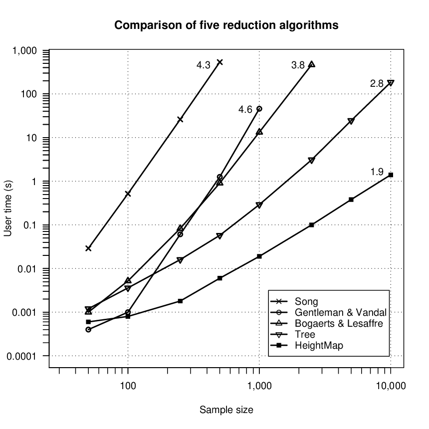
Table 1: Mean and standard deviation of the user time in seconds, over 50 simulations per sample size from model (4). Cells with NA indicate that simulations took over 1,000 seconds to run and were therefore omitted.

To get an empirical idea of the time complexity of the algorithms, Figure 3 shows a log-log plot of the mean user time versus the sample size. We fitted least squares lines through the last 4 points of each algorithm. The slopes of these lines can be used as empirical estimates of the time complexity of the algorithms. We see that the estimated slope of the HeightMap algorithm is 1.9, which agrees with the theoretical time complexity of $O(n^{2})$ that we derived earlier. Furthermore, we see that the HeightMap algorithm is about an order faster than the Tree algorithm, which is about an order faster than the algorithm of Bogaerts and Lesaffre. Finally, note that the empirical time complexity of the algorithm of Bogaerts and Lesaffre is greater than the theoretical complexity of $O(n^{3})$ that they derived.

4 MULTIVARIATE HEIGHTMAP ALGORITHM

The height map algorithm can be easily generalized to higher dimensional data. For example, for 3-dimensional interval censored data the observation sets $R_{i}$ take the form of 3-dimensional blocks $(x_{1,i},x_{2,i},y_{1,i},y_{2,i},z_{1,i},z_{2,i})$ . In this situation the height map is a function $h:\mathbb{R}^{3}\to\mathbb{N}$ , where $h(x,y,z)$ is the number of observation sets that contain the point $(x,y,z)$ . The maximal intersections again correspond to local maxima of the height map. By first transforming the observation sets into canonical sets, this implies that we need to find the local maxima of a $2n\times 2n\times 2n$ matrix. We can do this by sweeping through the matrix, slice by slice, say along the $z$ -coordinate. We only store one slice of the height map at a time, so that $h$ and $e$ are now $2n\times 2n$ matrices. At each step in the sweeping process, we either enter or leave an observation set $R_{i}$ . When we enter an observation set, we update the corresponding values of $h$ and $e$ , i.e. we set $h_{k,l}:=h_{k,l}+1$ and $e_{k,l}:=i$ for all $k=x_{1,i}+1,\dots,x_{2,i}$ and $l=y_{1,i}+1,\dots,y_{2,i}$ . When we leave an observation set, we look for local maxima in the cells of the rectangle $(x_{1,i},x_{2,i},y_{1,i},y_{2,i})$ , using the height map algorithm for 2-dimensional data. For each local maximum that we find, we check whether $e_{k,l}>0$ for all of its cells. If this is the case, we output the corresponding maximal intersection and set $e_{k,l}:=0$ for one of the cells in the local maximum. Finally, we decrement $h_{k,l}$ by 1 for $k=x_{1,i}+1,\dots,x_{2,i}$ and $l=y_{1,i}+1,\dots,y_{2,i}$ .

For $d$ -dimensional data, the time complexity of a sweeping step is $O(n^{d-1})$ . Since the number of sweeping steps is $O(n)$ , this gives a total time complexity of $O(n^{d})$ . With respect to the space complexity, we need to store the matrices $h$ and $e$ . Hence, the space complexity to compute the maximal intersections is $O(n^{d-1})$ . However, storing the maximal intersections takes $O(n^{d})$ space.

ACKNOWLEDGEMENTS

This research was partly supported by NSF grant DMS-0203320. The author would like to thank Kris Bogaerts, Shuguang Song, and Alain Vandal for providing the code of their algorithms, and a referee for suggesting to consider generalizing the HeightMap algorithm to $d$ -dimensional data. Finally, the author would like to thank Piet Groeneboom, Steven Schimmel and Jon Wellner for their contributions, support and encouragement.

APPENDIX: PSEUDO CODE

Algorithm 1: CompareEndpoints( $A$ , $B$ ):
Input: Two endpoint descriptors $A=(x_{k,i},c^{x}_{k,i})$ and $B=(x_{l,j},c^{x}_{l,j})$
Output: A boolean value indicating $A<B$
1:

$c_{A}:=(c^{x}_{k,i}=1)$ { boolean indicating $A$ is a closed endpoint}
2:

$c_{B}:=(c^{x}_{l,j}=1)$ { boolean indicating $B$ is a closed endpoint}
3:

$r_{A}:=(k=2)$ { boolean indicating $A$ is a right endpoint}
4:

$r_{B}:=(l=2)$ { boolean indicating $B$ is a right endpoint}
5:
if ( $x_{k,i}\neq x_{l,j}$ ) then { if the endpoints have different coordinates}
- 6:
  
  return ( $x_{k,i}<x_{l,j}$ ) { …then let their coordinates determine their order}
7:
if ( $r_{A}=r_{B}$ and $c_{A}=c_{B}$ ) then { if the endpoints are identical}
- 8:
  
  return ( $i<j$ ) { …then let their index determine their order}
9:
if ( $r_{A}\neq r_{B}$ and $c_{A}\neq c_{B}$ ) then { if the endpoints are opposites}
- 10:
  
  return ( $r_{A}$ ) { …then $A<B$ when $A$ is a right endpoint}
11:

return $(r_{A}\neq c_{A})$ { otherwise $A<B$ when $A$ is closed left or open right}

Algorithm 3: HeightMapAlgorithm2D( $R_{1},\dots,R_{n}$ ):
Input: A set of $n$ 2-dimensional observation rectangles $R_{1},\dots,R_{n}$
Output: The corresponding maximal intersections $A_{1},\dots,A_{m}$
1:

Transform observation rectangles into canonical rectangles $(x_{1,i},x_{2,i},y_{1,i},y_{2,i})$ , using CompareEndpoints
2:

Sort $x_{1,i},x_{2,i}$ , $i=1,\dots,n$ in ascending order and store their indices $i$ in the list $r_{1},\dots,r_{2n}$
3:

$m:=0$ { counts number of maximal intersections}
4:

$h_{1},\dots,h_{2n}:=0$ { column of height map}
5:

$e_{1},\dots,e_{2n}:=0$ { index of last entered rectangle; 0 blocks output}
6:
for $j=1$ to $2n$ do { sweep through height map from column $1$ to $2n$ }
- 7:
  if ( ${r_{j}}$ is a left boundary) then { we enter a rectangle}
  - 8:
    
    for $k=y_{1,r_{j}}+1$ to $y_{2,r_{j}}$ do { update $h_{k}$ and $e_{k}$ for $k=y_{1,r_{j}}+1,\dots,y_{2,r_{j}}$ }
    
    9:
    
    $h_{k}:=h_{k}+1$ ; $e_{k}:=r_{j}$
- 10:
  else { we leave a rectangle}
  - 11:
    
    $b:=y_{1,r_{j}}$ { bottom coordinate of local maximum; 0 blocks output}
  - 12:
    
    for $k=y_{1,r_{j}}+1$ to $y_{2,r_{j}}-1$ do { look for local maxima in rows $y_{1,r_{j}}+1,\dots,y_{2,r_{j}}-1$ }
    
    13:
    
    if ( $h_{k+1}<h_{k}$ and $b>0$ ) then { there is a local maximum in $h$ }
    
    14:
    
    if $(e_{b+1},\dots,e_{k}>0)$ then { the local maximum in $h$ is a maximal intersection}
    
    15:
    
    $m:=m+1;\quad A_{m}:=(x_{1,e_{k}},j,b,k)$ { output the maximal intersection}
    
    16:
    
    $e_{b+1}:=0$ { set $e$ to zero for row $b+1$ in $A_{m}$ }
    
    17:
    
    $b:=0$
    
    18:
    
    if ( $h_{k+1}>h_{k}$ ) then
    
    19:
    
    $b:=k$
  - 20:
    
    $k:=y_{2,r_{j}}$ { look for local maximum in row $y_{2,r_{j}}$ }
  - 21:
    
    if ( $b>0$ ) then { there is a local maximum in $h$ }
    
    22:
    
    if $(e_{b+1},\dots,e_{k}>0)$ then { the local maximum in $h$ is a maximal intersection}
    
    23:
    
    $m:=m+1;\quad A_{m}:=(x_{1,e_{k}},j,b,k)$ { output the maximal intersection}
    
    24:
    
    $e_{b+1}:=0$ { set $e$ to zero for row $b+1$ in $A_{m}$ }
  - 25:
    
    for $k=y_{1,r_{j}}+1$ to $y_{2,r_{j}}$ do { update $h_{k}$ for $k=y_{1,r_{j}}+1,\dots,y_{2,r_{j}}$ }
    
    26:
    
    $h_{k}:=h_{k}-1$
27:

Transform the canonical maximal intersections $A_{1},\dots,A_{m}$ back to the original coordinates
28:

return $A_{1},\dots,A_{m}$

References

Betensky and Finkelstein (1999 Betensky, R. A. and Finkelstein, D. M. (1999). “A Nonparametric Maximum Likelihood Estimator for Bivariate Censored Data,” Statistics in Medicine, 18, 3089–3100.
Bogaerts and Lesaffre (2004 Bogaerts, K. and Lesaffre, E. (2004). “A New Fast Algorithm to Find the Regions of Possible Support for Bivariate Interval Censored Data,” Journal of Computational and Graphical Statistics, 13, 330–340.
Gentleman and Geyer (1994 Gentleman, R. and Geyer, C. J. (1994). “Maximum Likelihood for Interval Censored Data: Consistency and Computation,” Biometrika, 81, 618–623.
Gentleman and Vandal (2001 Gentleman, R. and Vandal, A. C. (2001). “Computational Algorithms for Censored-Data Problems using Intersection Graphs,” Journal of Computational and Graphical Statistics, 10, 403–421.
Gentleman and Vandal (2002 ———— (2002). “Nonparametric Estimation of the Bivariate CDF for Arbitrarily Censored Data,” The Canadian Journal of Statistics, 30, 557–571.
Groeneboom and Wellner (1992 Groeneboom, P. and Wellner, J. A. (1992). “Information Bounds and Nonparametric Maximum Likelihood Estimation,” Birkhäuser, Boston.
Lee (1983 Lee, D. T. (1983). “Maximum Clique Problem of Rectangle Graphs,” Advances in Computing Research, 1, 91–107.
Song (2001 Song, S. (2001). “Estimation with Bivariate Interval Censored data,” Ph.D. thesis, University of Washington.
Turnbull (1976 Turnbull, B. W. (1976). “The Empirical Distribution Function with Arbitrarily Grouped, Censored, and Truncated Data,” Journal of the Royal Statistical Association, Ser. B, 38, 290–295.
Van der Vaart and Wellner (2000 Van der Vaart, A. W. and Wellner, J. A. (2000). “Preservation Theorems for Glivenko-Cantelli and Uniform Glivenko-Cantelli Classes,” High Dimensional Probability II, 115–133, Birkhäuser, Boston.
Wong and Yu (1999 Wong, G. Y. and Yu, Q. (1999). “Generalized MLE of a Joint Distribution Function with Multivariate Interval-Censored Data,” Journal of Multivariate Analysis, 69, 155–166.

Reduction Algorithm for the NPMLE for the Distribution Function of Bivariate Interval Censored Data