Quantum transport theory with nonlocal coherence
DEPARTMENT OF PHYSICS
UNIVERSITY OF JYVÄSKYLÄ
RESEARCH REPORT No. 3/2009
QUANTUM KINETIC THEORY WITH NONLOCAL COHERENCE
BY
MATTI HERRANEN
Academic Dissertation
for the Degree of
Doctor of Philosophy
To be presented, by permission of the
Faculty of Mathematics and Natural Sciences
of the University of Jyväskylä,
for public examination in Auditorium FYS-1 of the
University of Jyväskylä on June 12, 2009
at 12 o’clock noon
![[Uncaptioned image]](0906.3136v1/soihtu.png)
Jyväskylä, Finland
May 2009
Preface
The work reviewed in this thesis has been carried out during the years 2005-2009 at the Department of Physics in the University of Jyväskylä.
I am most grateful to my supervisor Doc. Kimmo Kainulainen for excellent guidance and support during these years. I have been privileged to share his profound ideas and wide knowledge of particle physics and cosmology. A major part of this work has been done in collaboration with Pyry Rahkila, to whom I want to extend my warmest thanks. I also want to express my gratitude to Prof. emer. Vesa Ruuskanen who introduced me to Kimmo many years ago, and to Prof. Mikko Laine and Prof. Kari Rummukainen for careful reading of the manuscript and valuable comments. I also wish to thank the staff and friends at the Department of Physics for creating an inspiring and pleasant working atmosphere.
The financial support from the Jenny and Antti Wihuri foundation, the Finnish Cultural Foundation, the Graduate School of Particle and Nuclear Physics (GRASPANP), and the Helsinki Institute of Physics (HIP) is gratefully acknowledged.
Finally, I wish to thank Jenni and my family for their love, support and patience.
List of publications
This thesis is based on the work contained within the following publications:
- I
Towards a kinetic theory for fermions with quantum coherence
M. Herranen, K. Kainulainen and P. M. Rahkila,
Nucl. Phys. B 810 (2009) 389 [arXiv:0807.1415 [hep-ph]]. - II
Quantum kinetic theory for fermions in temporally varying backgrounds
M. Herranen, K. Kainulainen and P. M. Rahkila,
JHEP 0809 (2008) 032 [arXiv:0807.1435 [hep-ph]]. - III
Kinetic theory for scalar fields with nonlocal quantum coherence
M. Herranen, K. Kainulainen and P. M. Rahkila,
JHEP 0905 (2009) 119 [arXiv:0812.4029v2 [hep-ph]].
The author has participated equally with K .Kainulainen and P. M. Rahkila in the development of papers I-III. A large part of the analytical calculations, in particular in papers II and III, was carried out by the author. The draft versions of papers II and III were largely written by the author.
Chapter 1 Introduction
A wide range of problems in modern high energy physics and cosmology involves the dynamics of quantum fields in highly out-of-equilibrium conditions, including relativistic heavy ion collisions [1, 2, 3], quantum fluctuations in inflationary cosmology [4, 5, 6], preheating after inflation [6], and baryogenesis [7]. It turns out that the traditional methods of (vacuum or thermal) quantum field theory (QFT) are not suited to describe these complicated non-thermal processes, and a new framework of nonequilibrium QFT [8, 9] is needed. Even though a knowledge of the complete dynamics of interacting quantum fields is clearly beyond reach, there is a variety of approximative methods that are able catch the essentials of the problems under study. In a so called kinetic regime with weak interactions and slowly varying classical backgrounds the standard methods of quantum kinetic theory reduce the problem considerably to solving the famous (quantum) Boltzmann transport equations. For many problems of interest these transport equations provide a remarkably good approximation for the essentials of nonequilibrium quantum dynamics. However, certain problems are inherently very sensitive to quantum coherence (or interference), quantum reflection from a potential being a typical example. The Boltzmann equation approach inevitably loses the effects of nonlocal quantum coherence, and thus is not very well suited to study for example the quantum reflection problem in electroweak baryogenesis or the particle production in preheating.
In this thesis we present a novel approximation scheme related to the quantum kinetic theory, that enables us to treat nonlocal quantum coherence in the presence of decohering collisions with simple enough Boltzmannian-type transport equations. The key element in our scheme is the finding of new singular shell solutions in the phase space of 2-point correlation function, that are located at for spatially homogeneous problems and at for a static planar symmetric case. When the complete phase space structure, including these new coherence solutions in addition to the standard mass-shell contribution, is inserted in the Kadanoff-Baym (KB) equations for the correlator, we obtain a closed set of transport equations for the corresponding on-shell distribution functions, thus giving an extension to the standard quantum Boltzmann equation to include nonlocal coherence.
The thesis consists of three original research papers [I]-[III] and an introductory and summary part presented below. In chapter 2 we introduce the basic mechanisms of (electroweak) baryogenesis and preheating, that are good examples of highly nonequilibrium processes in the early universe. In chapter 3 we present the basic formalism of nonequilibrium QFT needed to derive the KB-equations for two point correlation functions, using the two-particle irreducible (2PI) effective action method. Chapter 4 then presents a detailed survey of the main contents of our work, the novel approximation scheme. In chapter 5 we review a few applications that we have so far considered using our formalism, including the Klein problem, (collisionless) quantum reflection from a -violating mass wall, and examples of coherent production of decaying fermionic and scalar particles relevant for preheating. Finally, chapter 6 contains conclusions and outlook.
Chapter 2 Nonequilibrium processes in the early universe
According to modern theories of cosmology and particle physics the expanding universe has once been in an extremely dense and hot state (Hot Big Bang scenario), consisting of quantum plasma, which during the major part of the early evolution is very close to thermal equilibrium. Besides this overall picture of thermal plasma, however, many crucial processes in the early universe are inherently highly non-thermal, including inflation, preheating, and baryogenesis. The careful understanding of these processes is of primary importance in modern cosmology, providing an important field of applications to the methods of nonequilibrium quantum field theory. In this chapter we introduce the basic mechanisms of baryogenesis, focusing on a model called electroweak baryogenesis (EWBG), and the process of preheating after inflation.
2.1 Baryogenesis
The visible matter content of the universe, such as planets, stars and interstellar gas, consists of protons, neutrons and electrons. In astrophysics it is classified as baryonic matter, since the bulk of the mass is in protons and neutrons that are baryons. There is strong evidence that no large domains of antimatter exists in the universe [10, 11], implying that the universe has an excess of baryons compared to antibaryons which is called baryon asymmetry. The combination of data including several experiments of the fluctuations of cosmic microwave background (CMB) gives the following experimental measure of this asymmetry, the average baryon to photon number ratio in the universe [12]:
| (2.1) |
Of course it might be possible that the baryon asymmetry is an initial condition in the evolution of the universe. Despite being very unnatural, this explanation for the baryon asymmetry is not consistent with the cosmological inflation [4, 5], which is one of the backbones of modern cosmology explaining the homogeneity and flatness of the universe as well as the primordial density fluctuations that will give rise to structure formation and the observed fluctuations in the CMB spectrum. The problem is that the exponential increase in the size of the universe by at least a factor during the inflationary period dilutes any prior baryon number to totally negligible level. For this reason, we are very tempted to seek out different ways of creating the baryon asymmetry in the universe after the period of inflation.
A process that gives rise to a permanent baryon asymmetry at cosmological scales is called baryogenesis. The idea of such a process originates from Sakharov [13], who presented three conditions that any model for baryogenesis should necessarily fulfill:
- 1.
Baryon number violation.
- 2.
and symmetry violations.
- 3.
Departure from thermal equilibrium.
The first condition is obvious. If the second is not fulfilled, then for every reaction producing particles there is a counter-reaction that produces antiparticles at the same rate. The third condition is the most interesting for the scope of this work. It follows from the -theorem that the masses of particles and antiparticles are equal, and consequently the thermal average of the baryon number will vanish in equilibrium. We conclude that every scenario for baryogenesis must be a nonequilibrium process.
Several models for baryogenesis have been proposed that fulfill the Sakharov conditions (for a recent review see e.g. . [7]), including GUT baryogenesis [4], electroweak baryogenesis [14], leptogenesis [15] and Afflect-Dine baryogenesis [16] as the most prominent candidates. The first of these, GUT baryogenesis, is based on decays of heavy gauge bosons with masses of order . While it provides a scenario fulfilling all the Sakharov conditions, it has serious problems with inflationary models related to the high reheating temperature required, and the consequent overproduction of gravitinos [7]. The latter models, electroweak baryogenesis, leptogenesis and some variants of Affleck-Dine baryogenesis are based (directly or indirectly) on electroweak baryon number violation [17], which is a quantum anomaly in the electroweak sector of the standard model allowing the baryon number to be badly violated at high temperatures. These models differ however substantially in the mechanisms of how the required out-of-equilibrium conditions are reached. In what follows we will focus on EWBG in more detail, trying to elaborate the basic mechanism and the necessity to use the methods of nonequilibrium quantum field theory in its study.
2.1.1 Electroweak baryogenesis
Electroweak baryon number violation
Baryon and lepton numbers are classically conserved in the standard model. However, at the quantum level this is not the case. It can be shown that the axial current in the electroweak sector of the standard model and consequently the total baryon and lepton number currents and are anomalous i.e. not exactly conserved [18, 19]:
| (2.2) |
where is the number of fermionic families, and are the field strength tensors of the and gauge symmetries with the duals and an analogous expression for , and and are the associated coupling constants, respectively. Equation (2.2) implies that the total change in baryon (lepton) number from time to some arbitrary final time is given by:
| (2.3) |
where
| (2.4) |
are called the Chern-Simons numbers of the and gauge symmetries. We proceed by considering the vacuum structure of the gauge fields and . It turns out that the abelian sector has a trivial nondegenerate vacuum with , but the sector instead has a discrete set of degenerate vacua with
| (2.5) |
where , is an integer and are the generators of the gauge group. Using the vacuum structure Eq. (2.5) in Eqs. (2.3)-(2.4) we see that the change in baryon number in transitions between the different vacua is given by
| (2.6) | |||||

We see that the baryon number changes in integer multiples of in the transitions between different vacua. The structure of the effective potential for the gauge fields is sketched in Fig. 2.1, where the minima correspond to different vacuum configurations labelled by the (integer) Chern-Simons number . But how could the transitions between different vacua actually take place? At zero temperature the only possibility is by quantum tunneling through the potential barrier. This corresponds to the so called instanton configuration [17], but it turns out that the tunneling rate is negligible: . With this rate not a single proton could have been produced in the lifetime of the universe! At high temperature the situation is better. The transitions between the vacua can take place through a thermal activation over the potential barriers, via the so called sphaleron field configuration [20, 21]. The thermal transition rate corresponding to this process is shown to be [14, 22]
| (2.7) |
where is the energy of the sphaleron configuration, which is related to the vacuum expectation value of the Higgs field by . This result is valid only in the broken phase i.e. when the gauge symmetry is spontaneously broken and the gauge bosons are massive. In the symmetric phase with massless gauge bosons the sphaleron rate is instead given by (in the minimal standard model) [23]
| (2.8) |
where is the weak coupling constant. To see if the sphaleron transitions are fast at the time scales of the expanding early universe, the sphaleron rate of a unit comoving volume: , needs to be compared with the Hubble expansion rate of the (radiation dominated) universe [4]
| (2.9) |
where counts the total number of effectively massless degrees of freedom and is the Planck mass. In the minimal standard model at high temperatures of order GeV we have so that the symmetric phase sphaleron rate in Eq. (2.8) is very large compared to the Hubble rate. Moreover, if then also the broken phase sphaleron rate in Eq. (2.7) is large, and the first Sakharov condition is fulfilled in both of the phases. Actually, it is crucial in EWBG that the broken phase sphaleron rate is smaller than the Hubble rate so that the the generated baryon asymmetry is not washed out. Next we will briefly consider the electroweak phase transition between the symmetric and broken phases, where the gauge bosons and fermions become dynamically massive. This transition takes place at the (electroweak) temperature scale GeV, and it provides a scheme for the creation of a permanent baryon asymmetry through EWBG, if the transition is of first order.
Electroweak phase transition
In the electroweak theory of the standard model [24, 25, 26] the masses of the gauge bosons and and all fermions are generated through spontaneous symmetry breaking of the gauge symmetry . The “classical” potential of the ( doublet) Higgs scalar field :
| (2.10) |
where , is minimized for corresponding to a degenerate set of vacuum configurations. Choosing a particular vacuum from this set breaks the gauge symmetry spontaneously giving rise to masses for the gauge bosons, which are proportional to the vacuum expectation value of the Higgs field. This is how the Higgs mechanism works at zero temperature.
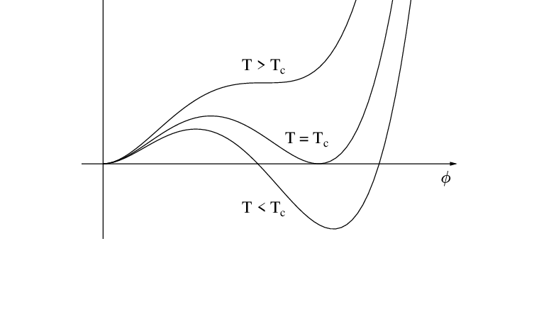
At finite temperatures the “classical” Higgs potential Eq. (2.10) gets temperature dependent quantum corrections that will become more and more important when the temperature increases. These corrections are taken in account by computing the free energy (or the effective potential) of the Higgs field [7]:
| (2.11) |
where the values of the parameters , and depend on the considered model. We have only given the dominant terms from perturbative calculations. The temperature dependence of the potential Eq. (2.11) gives rise to an interesting behaviour of the Higgs field. Let us first consider the case with vanishing third order term : when the second order term is positive implying that the minimum of the potential and the corresponding vacuum expectation value (VEV) of the Higgs field is zero: , while for it is finite: , since the negative second order term dominates for small . At the critical temperature there will be a phase transition from the former symmetric phase to the latter broken phase. This is called electroweak phase transition, and for the case it is a second order transition with smoothly increasing VEV as the temperature decreases. The case with presented in Fig. 2.2 is more interesting for us. At the critical temperature there is now a potential barrier between the symmetric and broken minima. Because of this barrier the phase transition actually takes place at a lower temperature , and latent heat is released due to the energy difference between the minima. Hence the transition is of first order and it happens by nucleation of broken phase bubbles inside the symmetric phase bulk. These bubbles start to grow rapidly reaching soon a stationary expansion speed. This scenario with first order phase transition is of crucial importance for the electroweak baryogenesis. It is just around the edge (or wall) of these broken phase bubbles where the last two Sakharov conditions of violation and departure from thermal equilibrium are fulfilled. Unfortunately, it has been shown by nonperturbative lattice calculations that for the minimal standard model the phase transition is not of first order [27]. For this and other reasons (e.g. not enough violation) we have to seek new possibilities for electroweak baryogenesis in extensions of the standard model, such as the minimal supersymmetric standard model (MSSM). Next we will give a brief conceptual description of the mechanism of (eletroweak) baryogenesis for a generic model with a strong first order phase transition.
Description of the EWBG mechanism

In Fig. 2.3 we present a schematic cross-section from the expanding bubble wall front where baryogenesis takes place. In the bubble wall region the VEV of the Higgs field and consequently the masses of the fermions (green line) are spatially dependent changing smoothly from zero in the symmetric phase to a finite value in the broken phase. The varying complex mass of a fermionic eigenstate gives rise to the required violating effects that will generate an asymmetry in left chiral number densities between particles and antiparticles (yellow line). This source asymmetry then creates a pseudo chemical potential that biases the sphaleron transitions in front of the wall in the symmetric phase to produce more baryons than antibaryons. This net baryon number is not washed away in the broken phase, because the sphaleron rate (red line) is too small there compared to the Hubble expansion rate . At the end, when the bubble wall has passed and the plasma is back in thermal equilibrium, a net baryon number density has been created.
One of the most difficult problems in the actual calculations of the baryon asymmetry is to find out the source asymmetry due to the violating effects. An accurate calculation would necessarily involve the use of nonequilibrium quantum field theory, and this is the background motivation for our work. In earlier works the problem has been studied in the semiclassical WKB approach [28, 29, 30, 31, 32, 33] and later with the methods of quantum kinetic theory in [34, 35, 36, 37, 38], both approaches using the Boltzmann transport equations for -violating phase space densities. These methods should provide a solid approximation in the semiclassical limit i.e. the case of a thick wall compared to the mean free path of the interacting fermions. However, in the thin wall limit the dominant source for the asymmetry comes from the quantum reflection processes, which are inherently nonlocal and absent in the standard WKB and kinetic approaches. Attempts have been made to treat the reflection phenomena by including collisions in the Dirac equation [39, 40, 41, 42, 43], but no consistent framework based on quantum field theory has been introduced. In this work we present an approximation scheme based on the kinetic approach that enables us to treat the quantum reflection in a simple but consistent way in the presence of decohering collisions.
2.2 Preheating
Cosmological inflation [44, 45, 46, 47, 48, 49, 50, 51, 52, 4, 5] (for a recent review see e.g. [6]) is a period of rapid exponential expansion in the very early universe during which the size of the universe increases by a huge factor (at least ). As mentioned in the beginning of last section, it provides a natural explanation for the homogeneity (horizon problem) and flatness of the universe. It also explains the (almost) scale invariant primordial density fluctuations that will give rise to large-scale structure formation and the observed anisotropies in the CMB spectrum [12]. Most of the inflationary models are based on the peculiar dynamics of one or several scalar fields, called inflaton(s), whose vacuum condensate dominates the evolution of the universe in a so called ‘‘slow roll’’ phase, causing the exponential growth. Because of the huge and very rapid expansion the universe is typically11 1 The warm inflation scenario with particle production during inflation is an exception [53, 54]. in a highly non-thermal and very cold state at the end of inflation. However, the baryogenesis scenarios require energies greater than the electroweak scale and the primordial nucleosynthesis requires that the universe is close to thermal equilibrium at the temperature MeV at some stage after inflation. A mechanism for reheating the universe after inflation is thus needed to retain the Hot Big Bang scenario.
The modern scenarios of reheating consist of a preheating stage followed by thermalization. In the preheating stage [55, 56, 57, 58, 59, 60] the inflaton condensate goes through rapid oscillations, so that the couplings to other matter fields give rise to particle production via parametric resonance. The basic mechanism is simple: the coupling to the inflaton(s) gives rise to rapidly oscillating effective masses for the matter fields that will bump up the particle numbers exponentially for certain momentum modes in close analogy with the Floquet theory of growing exponents [61, 62]. The modes in these resonance bands will quickly obtain huge occupation numbers (for scalars with no Fermi blocking). This rapid growth of perturbations is followed by backreaction and rescatterings. Backreaction means the effects of the growing perturbations (particle production) back on the dynamics of the inflaton condensate. In most scenarios it will rather quickly shut off the inflaton oscillations (faster than the Hubble expansion rate of the universe) and consequently terminate the particle production. Before that the fluctuations of the inflaton field itself will grow and give rise to rescatterings i.e. couplings between different momentum modes leading to the growth of occupation numbers for non-resonance modes as well. When the oscillations of inflaton field shut off completely the preheating stage ends and the fields start to thermalize. This thermalization process can be very complex, including regimes of driven and free turbulence [63], which makes it difficult to estimate the final reheat temperature. Moreover, in certain cases the universe might enter a “quasi-thermal” phase with a kinetic equilibrium reached much before the full chemical equilibrium [64].
In addition to scalar particles, the parametric resonance during preheating may produce a significant amount of fermionic particles. This resonant production could possibly lead to dangerous relic abundances of problematic particles such as gravitinos [65, 66]. Fortunately, extensive studies have shown that gravitino over-production can be avoided during the preheating in realistic supersymmetric theories [67, 68, 69, 70, 71, 72, 73]. Another interesting aspect in the fermionic preheating is the possibility to generate heavy fermions with masses of order - GeV, that could be important in e.g. leptogenesis [74, 75]. In chapter 5 we will apply our approximation scheme with decohering interactions to study a simple model of fermionic preheating, during which the fermion is subjected to decays.
Chapter 3 Basic formalism of quantum transport theory
The standard methods of (vacuum or thermal) quantum field theory (QFT) are not well suited for the study of nonequilibrium quantum fields for several reasons. First of all, the basic quantities of interest in nonequilibrium QFT are expectation values of operators in contrast to transition amplitudes in the standard vacuum QFT, requiring the formal extension of the time variable into a closed time path with two different branches. Other specific issues in nonequilibrium QFT are related to for example secularity11 1 The standard perturbative approach suffers from secular terms giving rise to big late-time contributions in all orders of perturbation expansion, no matter how small the coupling constant is [76, 77, 78]. Heuristically, this can be seen in the sense that for a big enough for every (no matter how small). causing the complete failure of the standard perturbative expansion in many cases of interest [76, 77, 78]. In this chapter we introduce the basic concepts of nonequilibrium quantum field theory in order to derive the Kadanoff-Baym (KB) transport equations for fermions and scalar bosons. We start by introducing the closed time path formalism with four basic propagators. Then, we use the two-particle irreducible (2PI) effective action methods to derive the self-consistent (Schwinger-Dyson) equations of motion for the full 2-point correlation functions of the system, which we then write in the form of KB-equations. Finally, we list some physical observables that can be expressed in terms of these 2-point functions.
3.1 Closed time path formalism
The closed time path (CTP or Schwinger-Keldysh) formalism was developed by Schwinger [79] and Keldysh [80] and further refined by many influential works, including [81, 82, 83, 84, 85, 86, 87, 88, 89]. The basic idea of the formalism is simple: In order to study the expectation values instead of transition amplitudes by the methods of quantum field theory, the time coordinate must be extended to a closed time path from initial time to final time (often taken to be ) and then back to 22 2 For this reason the CTP formalism is often called “in-in” formalism on the contrary to the traditional “in-out” formalism of quantum field theory with transition amplitudes between incoming and outgoing states. (see Fig. 3.1). The need for this closed time path can be demonstrated by writing the expectation value of a real scalar field in a state defined by arbitrary density operator in terms of a path integral (we choose here ):
where is the initial density matrix and the subscript denotes an operator in the Schrödinger picture in contrast to the Heisenberg picture without a subscript. We see that the path integral representation involves two “histories”, for which the evolution is chronological from to and antichronological from to , respectively. The field values in these / branches are independent except the boundary condition closing the path at , which we did not write explicitly in the last row of Eq. ().

3.1.1 Propagators
It turns out that the higher -point Green’s functions of the system will automatically become time ordered along the closed time path. Of special interest in quantum field theory are the 2-point functions or propagators, which are now defined as
| (3.2) | |||||
| (3.3) |
for a real scalar field and a fermionic field , respectively. is some unknown quantum density operator describing the statistical properties of the system, and defines the time ordering along the closed time path , shown in Fig. 3.1, in the sense that the points on the lower (negative) branch are “later” than those on the upper (positive) branch. When written in terms of the ordinary real time variable running from to , the closed time path propagators (3.2)-(3.3) contain four distinct contributions depending on the time branches of the “complex” CTP-coordinates and . That is, using indices to label the positive/negative branches, the scalar propagators are decomposed as:
where now and are ordinary time coordinates. Similarly, for fermionic propagators we have:
Using the generic notation to denote fermionic/scalar popagators we see that and are the chronological (Feynman) and anti-chronological (anti-Feynman) propagators, respectively, while and are the so called Wightman functions. In our further analysis we are especially interested in the dynamics of these Wightman functions, which contain the essential thermal or out-of-equilibrium statistical information of the quantum system under study, in order to compute for example the expectation values of the number current and the energy momentum tensor .
Before we start to build the calculational scheme of the CTP formalism, let us introduce a few more Green’s functions, which are useful in the following analysis, and list some of their properties. First, we define the retarted and advanced propagators:
| (3.6) |
where now refers to bosons/fermions. The definitions (), () and (3.6) then imply that the propagators have the following hermiticity properties:
| (3.7) |
and further and . These latter identities for retarted and advanced propagators suggests to decompose them into hermitian and antihermitian parts:
| (3.8) |
The antihermitian part is called the spectral function. Based on Eqs. (3.6) it is easy to show that and obey the spectral relation:
| (3.9) |
3.2 Two-particle irreducible effective action
and Schwinger-Dyson equations
In a nonlinear quantum field theory, including the majority of the interacting theories, the 2-point correlation functions necessarily couple to higher order correlators and so on, to form an infinite Schwinger-Dyson hierarchy of equations analogous to Bogoliubov-Born-Green-Kirkwood-Yvon (BBGKY) hierarchy in classical statistical mechanics [9]. For this reason it is an impossible task to solve the 2-point correlators exactly; that would correspond to a full solution of the nonlinear QFT. A major paradigm in practical applications thus is to truncate this hierarchy (slave the higher order correlators) in an appropriate way. The truncation can be done in many ways, for example by a brute use of perturbation theory or a loop expansion. However, these standard methods do not generally provide a good approximation for out-of-equilibrium dynamics, because of several problems e.g. with secularity [78].
A way to evade these problems is a method of obtaining the (truncated) equations of motion from variational principles of increasing complexity. On the first level we obtain an equation of motion for the field expectation value only, in the next level to and 2-point function , and so forth. The effective action corresponding to the -th level of this hierarchy is called n-particle irreducible (nPI) effective action . The heuristic difference between the nPI-method and the standard perturbation theory is that in the latter the solutions are written as an expansion in a small parameter, say coupling constant, while in the former the equations themselves are expanded. This difference is of crucial importance in nonequilibrium quantum field theory; it is the very reason for the problems of e.g. secularity with the standard perturbation method. The truncation procedure using the nPI-method is practically feasible as it turns out that the higher order nPI effective actions become redundant, once the order of expansion is fixed. That is, for example in a loop expansion33 3 A loop expansion in the nPI effective action corresponds to an expansion of the equations, not to the perturbative expansion of the solutions. at -loop order all nPI effective actions with are equivalent. In addition to these reductions there may be further simplifications depending on special conditions, such as vanishing of the average field [78].
3.2.1 From a generating functional to 2PI effective action
In this work we will concentrate on the two-particle irreducible (2PI) effective action [90, 91, 92, 93, 94, 83, 88], which will lead to a self-consistent dynamics for the 2-point correlation function as well as the 1-point function . We show, following ref. [9], how the 2PI effective action and the corresponding equations of motion are derived for a real scalar field. For fermions we will only give the appropriate results. We start by defining 2PI generating functional on the closed time path:
| (3.10) |
where we use notation with a branch doublet , so that e.g. , and define a “metric” , so that and and repeated indices are summed over. The CTP action is defined as , and and are local and nonlocal Gaussian sources, respectively. We also use de Witt summation convention to leave out integrals in the notation for the source terms: and similarly for . All -point Green’s functions are obtained from through functional differentiation with respect to sources , while generates the connected -point functions. Especially, the average field44 4 This is usually called mean field, but in this work we have a different notion for mean field, explained later in chapter 4. is defined as
| (3.11) |
If we set after the variation, then is the physical expectation value without sources. The 2-point functions can be obtained form either through a double derivative with respect to or through a derivative with respect to the nonlocal source . For later purposes we use the latter way, and define the full propagators as
| (3.12) |
From the definition we see that i.e. it corresponds to fluctuations with respect to the average field, and thus it actually reduces to Eq. () only for vanishing average field (and vanishing sources). To proceed, we define the 2PI effective action as a double Legendre transformation of :
| (3.13) |
where it is understood that the sources and are eliminated through the relations between them and the correlators and arising from Eqs. (3.11)-(3.12). These relations are always invertible following from the general properties of Legendre transformation. The desired equations of motion for the correlators and are now obtained by functional differentiation:
| (3.14) |
so that in the case of physical (sourceless) dynamics we get the equations: and , which corresponds to finding the extremum for the effective action .
3.2.2 Formula for the 2PI effective action in terms of the fluctuation field
In order to use the equations of motion (3.14), we want to find a practical method to compute the 2PI effective action . To implement the so called background field method, we write the effective action in the form:
| (3.15) |
which follows directly from Eqs. (3.10) and (3.13). Here we have left out the initial density matrix contribution . The justification for this can be seen in two ways. First, if the initial state is Gaussian, the initial density matrix can be written as , and the new initial-time Kernel can be absorbed in the source . But this inclusion seems to ruin the desired condition that the physical evolution is given by vanishing sources and . However, since vanishes for all but initial time, we see that it affects only the initial conditions for the 1- and 2-point functions and , and hence can be neglected in the dynamical equations if we do adjust these initial conditions correctly [78]. The other possibility when the neglection of is justified is to consider such initial conditions, where the initial state in the distant past is in the in vacuum. This condition is implemented by just shifting the mass to in the first first branch and to in the second branch55 5 This is why the complex conjugate is explicitly written in the second branch action , even though the classical action is always real. i.e. “tilting” the time path in the complex plane in the same way as in the standard vacuum quantum field theory [9]. For an initial state that is neither of these cases the omitting of is not strictly justified and the following developments in this section provide only an approximation. If one wishes to consider those non-Gaussian initial states more accurately one needs to use higher nPI effective actions.
To come back to equation (3.15), we see that using Eqs. (3.14) and the symmetry of the source the exponent becomes
| (3.16) |
Next we shift the integration variable in Eq. (3.15) by the average fields: and expand the classical action in powers of the new fluctuation field :
| (3.17) |
where means functional derivatives of with respect to evaluated at and similarly for the second derivative , and denotes the collection of the higher order terms (cubic and so forth) in the fluctuation field . Furthermore, we separate the trivial (lowest orders) and nontrivial parts of by writing it in the form
| (3.18) |
where the infinite constant (often discarded since it does not affect the equations of motion) is and we denote 66 6 The motivation for this notation is that becomes the inverse free propagator in the limit of vanishing .. Plugging these expressions in Eq. (3.15) we find that the nontrivial part can be expressed as:
where
| (3.20) |
We see that despite the -term has the form of a generating functional for a new theory with classical action and sources and . Next we show that these sources with the additional term will just fix the 1- and 2-point functions of this new theory. To show that, we start by considering the matrix
| (3.21) |
which we know is invertible, because of the general invertibility of Legendre transformations. In terms of the derivatives of this becomes (also subtracting a singular matrix which does not affect invertibility)
| (3.22) |
On the other hand, by taking variational derivatives of Eq. () we get the equations
| (3.23) |
So, since the coefficient matrix is invertible, we conclude that
| (3.24) |
This result has tremendous implications: As the sources and just kill the 1-point function and fix the 2-point function to , it follows that we can neglect these sources in the practical calculations, if we include only the vacuum contribution77 7 In non-vacuum graphs the external legs are connected to the average field of -theory that vanishes to the effective action using as the full propagator of this -theory. Furthermore, because the full propagator is fixed to , it follows that in the diagrammatic calculations we need to consider only two-particle irreducible (2PI) graphs i.e. graphs that do not become disconnected while cutting two internal lines (see Fig. 3.2), hence the name for the 2PI action. So, we conclude that the 2PI effective action for the original theory is given, besides the terms explicit in equation (3.18) (classical and one-loop contribution), by the sum of all 2PI vacuum graphs in a theory with action . For example, for the real scalar field with quartic interaction:
| (3.25) |
where and the other components are zero, we find by performing the shift that the interaction part for the -theory is given by
| (3.26) |
Note that a cubic interaction with an effective vertex depending on the average field is generated.

3.2.3 Schwinger-Dyson equations for the propagators
Using the expression (3.18) for in the equations of motion (3.14) we get the following equation for the propagator in the (physical) case of vanishing sources:
| (3.27) |
where the second term follows from variation: . By defining the self energy:
| (3.28) |
we see that this equation (3.27) is of the form of famous Schwinger-Dyson equation for the full propagator:
| (3.29) |
which (upon inverting) is presented graphically in Fig. 3.3. To get this equation in a form that is feasible for practical calculations we multiply it from the right by to obtain
| (3.30) |
This is an integro-differential equation for the full propagator , because the inverse free propagator on the LHS contains explicit spacetime derivatives acting on , while on the other hand the full propagator appears inside the integral on the RHS, and also the self energy is (typically) a nontrivial functional of . One should stress that this Schwinger-Dyson equation is formally exact in the case of Gaussian (or distant past vacuum) initial conditions. However, the actual computation of the self energy via the 2PI action is a nontrivial task and in most cases of interest necessarily involves some truncation, such as the loop expansion or a large expansion for -invariant theories.

For fermions the construction of the 2PI effective action is very similar to scalar fields. However, due to the fact that fermionic fields are Grassmann numbers, there are some differences in the final formula, which for vanishing fermionic average field is given by [78]:
| (3.31) |
where is again the sum of two-particle irreducible vacuum graphs in the theory with propagator and the vertices are the same as in the original action, because of the vanishing average field. By comparing this with the scalar expression (3.18) we see a difference of a factor in the first two terms. This is due to different values of the functional determinant arising from the scalar and fermionic path integrals. In the same way as for scalar fields we obtain a completely analogous Schwinger-Dyson equation for the propagator :
| (3.32) |
where the self energy is now defined as:
| (3.33) |
Note that for a complex scalar field the 2PI effective action would be similar to the fermionic expression (3.31), without factors, but with different signs in the first two terms (see e.g. [37]). Consequently the definition of the self energy would be the same as in Eq. (3.33) except for the sign difference. The reason why the complex scalar field differs from the real one is basically just the doubling of the degrees of freedom for a complex field. Finally, we note that for an interacting theory that combines fermionic and scalar fields e.g. by a Yukawa interaction, we would just need to combine the nontrivial -parts of the 2PI effective actions and include contribution from the Yukawa interaction. This would naturally lead to cross-couplings in the fermionic and scalar Schwinger-Dyson equations.
3.3 Kadanoff-Baym transport equations
Let us use again the generic notation for fermionic and scalar propagators and denote both self energies simply by , and also adopt the same notation: etc., as for scalar and fermionic propagators Eqs. ()-(). It follows that the different components of Schwinger-Dyson equations (3.30) and (3.32) are consistent provided that the self energies can be divided in local (singular) and nonlocal parts
| (3.34) |
where the nonlocal part obeys similar relations as the propagators:
| (3.35) |
for scalars and fermions, respectively. These relations (3.34)-(3.35) should hold generally for any reasonable approximation of the self energy [37]. The singular term can be absorbed into the inverse propagator on the LHS of the Schwinger-Dyson equations either to the mass renormalization or to a classical background field (for example for gauge interactions). From now on we assume that this absorption is made and denote simply: . We further define the retarted and advanced self energies and their (anti)hermitian parts analogously to the propagators in Eqs. (3.6) and (3.8)88 8 The defined self energies clearly follow the hermiticity properties of the propagators, Eq. (3.7) and below. The antihermitian part is denoted as :
| (3.36) |
corresponding to the scattering width of the field excitations. For scalar fields Eq. (3.36) is conventionally defined as , when is directly the scattering width with the correct dimension. For fermions is a (spinor) matrix and the physical meaning of various elements is more obscure and will be discussed later in section 5.3 in the case of interaction with a thermal background.
Next we want to write the Schwinger-Dyson equations in a different form to make a separation between the dynamical and spectral properties of the system more evident. Using the above definitions and the corresponding ones for the propagators in Eqs. (3.6) and (3.8), and the fact that for vanishing average fields the inverse free propagator obeys , it is a matter of simple algebra to show that the Schwinger-Dyson equations (3.30) and (3.32) can be written in the form:
| (3.37) |
and
| (3.38) |
where, as stated before, we have assumed that the singular self energy is absorbed into , and we use the notation for the convolution integral:
| (3.39) |
The equations (3.37) are called pole equations, while Eq. (3.38) is one of the two Kadanoff-Baym (KB) equations [95]. The similar KB-equation for the other Wightman function needs not to be considered, since from the definition (3.8) it immediately follows that . In general, the pole equations will fix the spectral properties of the theory, while the KB-equations will give the dynamical evolution, i.e. the quantum transport effects. Indeed, in the classical limit the KB-equations (3.38) for fermions and scalars will reduce to well known quantum Boltzmann transport equations for the phase space number densities (see e.g. [9, 34, 36, 37, 38]).
3.3.1 Mixed representation and gradient expansion
If there is a clear separation between internal (microscopic) and external (macroscopic) scales in the system, it is appropriate to analyze the pole- and KB-equations (3.37)-(3.38) in so called mixed or Wigner representation, where a partial Fourier transformation with respect to the internal coordinate is performed. This transformation leads to a gradient expansion in derivatives of the external (average) coordinate , which contains, in general, infinitely many terms. However, if the separation of the scales is manifest, this expansion can be truncated (or resummed) to a good approximation.
To begin with, let us define the Wigner transformation for an arbitrary 2-point function :
| (3.40) |
where is the average coordinate, and is the internal momentum conjugate to the relative coordinate . Using this definition it is easy to transform the equations (3.37) and (3.38) into the mixed representation to get
| (3.41) | |||||
| (3.42) |
and
| (3.43) |
where the collision term in Eq. (3.43) is given by
| (3.44) |
and the -operator is the following generalization of the Poisson brackets:
| (3.45) |
The differential operators are related to the inverse propagators:
| (3.46) | |||||
| (3.47) |
for bosons/fermions respectively, where means that the derivative is acting on the left to . Note that these operators are not the transformed inverse propagators, but follow from the identity: .
Eqs. (3.41)-(3.43) are the desired quantum transport equations for the 2-point correlation functions , and . We are primarily interested in solving the Kadanoff-Baym equation (3.43) for the Wightman function , but in general, also the pole equations (3.41)-(3.42) have to be considered because of the cross-couplings between the equations. One can see that these equations indeed contain the derivatives of the masses and the self-energies up to infinite order, restraining their use in practical applications unless this gradient expansion can be truncated (or resummed) in some reasonable way.
In the standard approach to quantum kinetic theory the conditions of so called quasiparticle or on-shell approximation are assumed, including slowly varying (i.e. “nearly” translation invariant) background fields and correlators, as well as weak interactions [9]. This approach provide a consistent approximation to truncate the gradient expansion in KB-equations (3.43) to leading order, culminating in the derivation of the famous quantum Boltzmann equations. However, because of the assumptions made, it follows that the correlators whose dynamics we are studying, are “close” to local thermal equilibrium throughout the evolution. Especially the information on quantum coherence will be irrevocably lost. In the next chapter we start to build an extended approximation scheme that incorporates the good features of the standard kinetic approach with easy-to-use Boltzmannian-type transport equations, yet including the effects of nonlocal quantum coherence.
3.4 Physical quantities from 2-point correlation functions
We conclude this chapter by writing down some familiar physical observables, including the number currents and the energy momentum tensors for fermionic and scalar fields, in terms of the 2-point correlation functions and . These expressions follow directly from the definitions of the correlators in Eqs.(-) written in the mixed representation, so we simply list the results here. The expectation value of the fermionic number current is given by
| (3.48) |
and for complex99 9 No conserved Noether current can be defined for a real scalar field scalar bosons we have:
| (3.49) |
The symmetric (Belinfante) energy momentum tensor (see e.g. [96]) for fermions is
| (3.50) | |||||
while the bosonic tensor for real scalar field is given by
| (3.51) |
where is the standard Minkowskian metric with signature . For a complex scalar field we get a result with the last row of Eq. (3.51) multiplied by two. These relations demonstrate the importance of the 2-point Wightman functions in nonequilibrium quantum field theory. Later, in section 4.6 we will use these results to express the observables in terms of the on-shell distribution functions.
Chapter 4 Quasiparticle picture including nonlocal quantum coherence
4.1 Extended quasiparticle approximation
In the literature (see e.g. [97]) a quasiparticle approximation (QPA) usually refers to a set of approximations leading to a spectral phase space structure for the 2-point correlation functions , composed of sharp singular shells with definite energy momentum dispersion relations, such as the standard free particle mass shell. An alternative, stronger definition for QPA [9] requires that the functional forms of the free theory propagators are preserved in (QPA) interacting theory, with only the mass parameters replaced by effective masses. For both of these definitions the necessary conditions for the quasiparticle approximation to be justified include weak interactions and slowly varying background fields. Moreover, the standard treatment of QPA relies on the assumption that system be close to thermal equilibrium and consequently nearly translation invariant, the famous example being the derivation of the quantum Boltzmann transport equation from KB-equations [9].
Our extended quasiparticle approximation (eQPA) scheme relinquishes the assumption that the system needs to be close to thermal equilibrium. The key observation in our approach is that under the (otherwise) same conditions of QPA with weak interactions and slowly varying background fields, the phase space of the 2-point correlators contains novel and completely different singular shell solutions, in addition to the standard (quasi)particle mass-shell solutions. These new -shell solutions are unavoidably absent if we demand that the system is near thermal equilibrium, hence their lacking in the standard quasiparticle treatments. We will examine these new solutions in detail in section 4.3, where we interpret them as describing the nonlocal quantum coherence between “opposite” (quasi)particle excitations. After the complete spectral structure of the correlators is discovered, we feed it as an ansatz to the dynamical equations to find out the equations of motion for the corresponding on-shell distribution functions , including the novel coherence shells. In this way we get an extension to the quantum Boltzmann transport equation to include the effects of nonlocal quantum coherence.
First, we examine the necessary conditions for the extended quasiparticle approximation to be justified. These conditions include weak interactions, slowly varying background fields, and existence of particular spacetime symmetries. If some of these conditions are not fulfilled, the spectral approximation for the phase space breaks down. At the end of this section we outline the procedure of using the dynamical equations to find the desired equations of motion for the on-shell functions. The actual derivation of the appropriate equations for fermions and scalar bosons is presented in section 4.4.
4.1.1 Weak interactions
The limit of weak interactions in the context of quasiparticle approximation means in Eqs. (3.41)-(3.43), where is the interaction width defined in Eq (3.36). This limit is taken strictly whenever the phase space properties of the correlators are studied. However, when studying the dynamical properties, one has to include to at least leading order to get any thermalization effects. This is precisely the way how the Boltzmann transport equation is obtained in the classical limit.
Neglecting the terms proportional to in Eqs. (3.41)-(3.43), including the collision term (in general ), leads to the free field equations except for the self energies . It is not completely obvious how these self energies should be handled, however. For a controlled expansion in the coupling constant, all the self energies need to be treated in an equal footing; if we neglect , we have to neglect also at the same order. So, it would be justified to retain only if it is of lower order in coupling constant than . This is indeed the case for gauge interactions for example, with and in the lowest order. Another approach is to treat and completely independently, so that even if there is no coupling hierarchy, will be retained in the equations when the phase space properties of the correlators are examined. The motivation for this non-controlled approximation is that retaining will not ruin the spectral structure of the correlators; it merely modifies the dispersion relations of the excitations, so that the standard free particles become quasiparticles.
4.1.2 Slowly varying background, mean field limit
In general, it is not enough to neglect the terms proportional to to obtain a spectral phase space structure for the 2-point correlators. This can be demonstrated for a scalar field with nonvanishing constant , while other derivatives of the mass are vanishing. The spatially homogeneous solution for the free field ( is also neglected) KB-equation (3.43) is then:
| (4.1) |
where is the Airy-function. This is not a singular distribution in momentum for nonvanishing , but indeed in the limit it reduces to . This example illustrates that in order to obtain spectral phase space structure one needs to consider slowly varying background fields. Moreover, to actually get singular shell solutions all derivatives of the background field have to be neglected in the equations (3.41)-(3.43). This approximation of including only the zeroth order gradients of the background is called mean field (or adiabatic) limit. The resulting KB-equations for the study of the phase space properties of the correlators in combined weakly interacting and mean field limits are then
| (4.2) | |||||
| (4.3) |
for fermions and scalars, respectively. The corresponding pole equations are completely the same with replaced by on the RHS of the equations for .
4.1.3 Special spacetime symmetries
It turns out that even the mean field equations (4.2)-(4.3) do not in general have spectral solutions for the correlators. We see this by considering a dimensional free scalar field, for which the solution for Eq. (4.3) reads (for ) [98]:
| (4.4) |
where and are real functions of determined by the initial conditions, and is defined as:
| (4.5) |
This solution is not restricted to spectral form with support only on singular shells; instead it potentially has support everywhere inside the mass shell , or outside the light cone , depending on the unspecified functions and . For an arbitrary -dependence this is in conflict with the quasiparticle approximation, which requires that the phase space structure is spectral. However, if we demand for example the complete translational invariance: , then must be zero, implying that . We conclude that there can be support only on the mass shell, and the solution is indeed spectral. In the same way, if we demand only time translational invariance, , we find two different spectral solutions: the former mass-shell solution, but also a nonconstant solution in with . Later, in section 4.3, we examine the spectral phase space solutions in more detail with a different approach by subjecting the solutions of Eqs. (4.2)-(4.3) on certain spacetime symmetries in the first place. At least for fermions, this seems to be the only reasonable method, because of the complex spinor structure. In section 4.3 we will find that the phase space structure of fermionic and scalar correlators is indeed spectral for two particular spacetime symmetries of interest: spatial homogeneity and static planar symmetry.
4.1.4 Spectral ansatz for dynamical equations
The next step in our approximation scheme is to insert the spectral solutions as an ansatz in the full KB-equations (3.43). Now we are interested in the dynamics of the spectral solutions, so we will consider only those of the resulting component equations that include direct spacetime derivatives. We will resort to some approximations also in this step. As stated before, we are assuming the limit of weak interactions. However, now we do not want to neglect the terms proportional to completely, since that would lead to collisionless plasma dynamics. Instead we will include only the leading order terms in . To see which terms are actually leading order can be somewhat difficult in practice. It has been shown that for a scalar field close to thermal equilibrium, the term proportional to on the LHS of Eq. (3.43) is of higher order in than the dominant contribution from the collision term [37], so in this limit it is justified to neglect that term. For more general situations, however, it is not evident that neglecting this term would be justified by any simple arguments. For fermions this hierarchy has not been shown even for systems close to thermal equilibrium, as far as we know. Nevertheless, neglecting the term may anyway be a good first approximation; for example the well-known Boltzmann transport equation is derived in this limit. Further investigations on the role of this term (in dynamical equations) are definitely needed to make any conclusion on its importance.
The role of the term proportional to on the LHS of Eq. (3.43) poses another question. Clearly, if the mean field part has been included in the study of spectral properties in equations (4.2)-(4.3), the same term should be included in dynamical equations as well. The gradient corrections11 1 The higher gradient corrections in -terms do not necessarily correspond to gradients of the background field, and thus are not on the same footing as the overall mean field approximation to this term are yet another question, and in the sense of a controlled expansion in coupling constant, they should also be included. However, the role of these higher gradient contributions would probably be the same as the mean field contribution to i.e. to affect the spectral properties by “modifying” parameters like masses and momenta in the equations. By these arguments, neglecting higher gradient terms of when the dynamics of the spectral solutions are studied, seems to be quite well justified.
On the other hand, it is of course possible to include all of these interaction dependent terms in Eq. (3.43). Based on the above discussion, it is appropriate to do this by including everything else than the mean field contribution of formally into the collision term. The KB-equations for fermions and scalars then become
| (4.6) | |||||
| (4.7) |
where the “extended” collision terms are defined as
| (4.8) | |||||
| (4.9) |
The higher order gradients in the collision term are a delicate issue in our approximation scheme. Usually, when slowly varying backgrounds are studied and the solutions are close to thermal equilibrium, it is justified to neglect consistently all higher (than zeroth) order derivatives in collision term, since those will necessarily correspond to higher order gradients in the background field. However, in our scheme the coherence shell solutions are rapidly oscillating even in constant backgrounds, and consequently the higher derivatives in the collision terms do not necessarily correspond to higher order gradients in the background field and thus it is not a priori justified to neglect them. In practical calculations this gradient expansion has to be truncated, however, unless the different order gradients of the self energy terms can be resummed in some useful way. Later on in chapter 5, we show that this resummation is indeed possible for a scalar field interacting with a thermal background.
To summarize, our approximation scheme works as follows: First, we find out the spectral properties of the 2-point functions by using the weakly interacting mean field equations (4.2)-(4.3). Then, we substitute the obtained spectral solutions as an ansatz in the full interacting equations (4.6)-(4.7) (with the extended collision terms or the standard ones of Eq. (3.44)) to find out the equations of motion for the on-shell functions in the presence of collisions. The crucial difference compared with the standard treatment based on the quasiparticle approximation is that we do not assume that the system is close to thermal equilibrium at any moment, yet we are using the spectral solutions for the correlators. This apparent paradox will be settled in section 4.3, where we find the novel coherence shell solutions that have completely different properties than the standard (quasi)particle mass-shell solutions. In what follows, we will neglect the and terms on the LHS of Eqs. (4.6)-(4.7), since we are primarily interested in the general structure of the phase space and the dynamics of the on-shell functions, and not so much in the specific modifications of dispersion relations caused by interactions. Thus, while studying the phase space properties, the corresponding equations are effectively reduced to the noninteracting mean field limit.
4.2 Reduction of the spin structure in fermionic equations
Before we enter the study of the phase space shell structure, let us first simplify the fermionic KB-equation (4.6) further in the cases of two spacetime symmetries of interest: the spatial homogeneity and the static planar symmetry. To begin with, we write the equation (4.6) for the hermitian Wightman function, defined as
| (4.10) |
By multiplying both sides of Eq. (4.6) by we get
| (4.11) |
where we use the notation:
| (4.12) |
and we have dropped the tilde in the collision term to denote either the extended collision term in Eq. (4.9) or the standard one in Eq. (3.44).
4.2.1 Spatially homogeneous case, helicity diagonal
correlator
In a spatially homogeneous case the spatial gradients of and in Eq. (4.11) vanish, and consequently the helicity operator , where , commutes with the differential operator on the LHS of Eq. (4.11). This implies that different helicity projections
| (4.13) |
where denotes the helicity projector:
| (4.14) |
do not mix in a noninteracting theory22 2 By noninteracting theory we mean here that the self-energies and consequently the collision term are vanishing. The system still interacts with the varying classical background (giving rise to varying mass)., so that helicity is a good quantum number i.e. a conserved quantity. It follows that the helicity off-diagonals couple to the dynamics of the diagonal part only through the collision term. In this work we will not consider these cross-couplings, but use the helicity diagonal part of the correlator: , as an ansatz for the interacting theory. In the Weyl basis, where the gamma-matrices are given by the following direct product expressions (both and are the usual Pauli matrices referring here to chiral / spin d.o.f. respectively):
| (4.15) |
the helicity diagonal correlator can be written as:
| (4.16) |
where are (unknown) hermitian matrices (for ) in chiral indices. By taking a helicity diagonal projection of Eq. (4.11) we get then an equation for :
| (4.17) |
where the matrix is the chiral part of the helicity diagonal projection of the collision term:
| (4.18) |
Given that is a hermitian matrix, it is useful to decompose the equation (4.17) into hermitian (H) and antihermitian (AH) parts:
| (4.19) | |||||
| (4.20) |
where
| (4.21) |
can be interpreted as a local free field Hamiltonian operator, and are the hermitian and antihermitian parts of . We see that in the noninteracting mean field limit with and only the AH-equation contains an explicit time derivative of , while the H-equation is a purely algebraic matrix equation. For this reason the AH-equation is called a “kinetic equation” describing the dynamical evolution of the helicity diagonal Wightman function in a varying background. The H-equation on the other hand is called a “constraint equation”, which will constrain the solutions of the kinetic equation in the 4-dimensional phase space and thus is the one to be used in determining the phase space properties of the (eQPA) interacting theory.
4.2.2 Static planar symmetric case, spin- diagonal
correlator
In a static planar symmetric case all but one spatial derivative (chosen to be here) of and vanish. Then, apart from the -term, the differential operator on the LHS of Eq. (4.11) commutes with the spin in -direction: . We can proceed analogously to the previous section 4.2.1, by first performing a Lorentz boost to a frame where this term vanishes [34, 36, 37]. The Dirac representation of the desired boost is found to be
| (4.22) |
The boosted correlator33 3 Whereas transforms conventionally: , the hermitian correlator obeys a peculiar transformation law: .
| (4.23) |
then obeys an equation
| (4.24) |
where . After this boost the differential operator on the LHS of Eq. (4.24) indeed commutes with the spin , as expected. Analogously to the spatially homogeneous case this implies that different spin projections
| (4.25) |
where denotes the spin- projector:
| (4.26) |
do not mix in a noninteracting theory, so that spin- is a good quantum number. We again neglect the effects of spin off-diagonals and consider only the spin diagonal correlator, which is written in the Weyl basis as:
| (4.27) |
where are hermitian matrices (for ) in chiral indices. By taking the spin- diagonal projection of Eq. (4.24) we get now the following equation for :
| (4.28) |
where the matrix is the chiral part of the spin- diagonal projection of the boosted collision term:
| (4.29) |
Now, because the matrix is multiplying the derivative in Eq. (4.28), the straightforward division into hermitian and antihermitian parts does not lead to a convenient separation of the derivatives. However, by first multiplying Eq. (4.28) from the left by and only then taking the hermitian and antihermitian parts gives the desired division:
| (4.30) | |||||
| (4.31) |
where
| (4.32) |
and are the hermitian and antihermitian parts of . These equations are analogous to Eqs. (4.19)-(4.20) of the spatially homogeneous case. Again, the AH-equation is called a “kinetic equation” describing the dynamical -evolution of the spin diagonal Wightman function, while the H-equation is called a “constraint equation” determining the phase space properties of the correlator.
4.3 Phase space shell structure
We now begin to examine the phase space structure of the fermionic and scalar Wightman functions and in the (extended) quasiparticle limit discussed in section 4.1 for the case of . We find out that in addition to the standard mass-shell excitations, with the dispersion relation , the phase space consists of novel singular shell solutions that are located at for a spatially homogeneous case and at for a static planar symmetric case.
4.3.1 Fermions
As discussed above, the relevant equations that describe the phase space properties of the fermionic Wightman function are the constraint (H) equations Eqs. (4.19) and (4.30), that in the noninteracting mean field limit reduce to
| (4.33) | |||||
| (4.34) |
for the spatially homogeneous and the static planar symmetric cases, respectively.
Spatially homogeneous case
To further analyze the constraint equation (4.33) for the spatially homogeneous case, it is convenient to introduce the so called Bloch-representation for the chiral matrix :
| (4.35) |
where are the (chiral) Pauli matrices and are real functions, because of the hermiticity of . It is easy to see that in the Bloch-representation the constraint equation (4.33) decomposes into a simple homogeneous matrix equation
| (4.36) |
where the coefficient matrix is (index ordering is here defined as ):
| (4.37) |
A homogeneous matrix equation, such as Eq. (4.36), may have nonzero solutions only when the determinant of the matrix vanishes. Here the determinant is simply:
| (4.38) |
which implies that the nonzero solutions are possible only when
| (4.39) |
These constraints give rise to a singular shell structure for the solutions, since they need to be proportional to or . The former class is identified as the standard one particle mass-shell solutions, with the dispersion relation , while the latter class of solutions with are completely novel in the context of quantum field theory (see Fig. 4.1). Based on the observation that the quantum interference of the plane waves contains a contribution with , we make an interpretation that these additional ()-shell solutions describe the quantum coherence between the particles and antiparticles (positive and negative energy states) with opposite momenta and spin.

The explicit matrix structure of these solutions is found easily by setting and in the matrix equation (4.36) for the mass-shell and the coherence shell solutions, respectively [I]. The full chiral matrix corresponding to the mass-shell solution is given by:
| (4.40) |
where and are real functions parametrizing this solution. The on-shell distribution functions are called the phase space densities for positive and negative energy modes, respectively. Indeed, in the thermal limit they are related to the number densities of physical particles, as we will see later. For -shell solution we get on the other hand
where and are new undetermined real functions corresponding to the degrees of freedom of this coherence solution. The most general solution satisfying the constraint equation (4.33) (or equivalently the matrix equation (4.36)) for a spatially homogeneous case is the linear combination of Eqs. (4.40) and (4.3.1):
| (4.47) |
This general solution contains four independent on-shell distribution functions (for both ), which is just the number of independent components in a hermitian matrix, such as the chiral matrix . Indeed, in section 4.4 we find that there is a one-to-one mapping between these on-shell functions and the components of the -integrated chiral matrix .
Static planar symmetric case
The analysis of the static planar symmetric case proceeds in complete analogy. By introducing a Bloch representation for :
| (4.48) |
with real , the constraint equation (4.34) decomposes again into a homogeneous matrix equation
| (4.49) |
where the coefficient matrix is now (index ordering is again ):
| (4.50) |
The nonzero solutions of this matrix equation are found at the zeros of the determinant
| (4.51) |
which are now:
| (4.52) |
The former condition gives again the standard one particle mass-shell solutions, with , while the latter condition gives now a different novel class of solutions (see Fig. 4.2). By the same argument as in the spatially homogeneous case, we interpret that these additional ()-shell solutions describe the quantum coherence between the states of same spin and energy travelling in opposite z-directions.

The matrix structure of these solutions is found by setting (mass-shell) and (coherence shell) in the matrix equation (4.49). For the mass-shell solution we get
| (4.53) |
where and are real on-shell distribution functions parametrizing this solution. The coherence shell solution is given by
where and are new real distribution functions. The most general solution satisfying the constraint equation (4.34) for a static planar symmetric case is now the linear combination of Eqs. (4.53) and (4.3.1):
| (4.60) |
In this case also, we later find that the four independent on-shell functions will uniquely correspond to the components of the integrated chiral matrix , where the integration is now over instead of .
We later see that even in the simplest possible example of constant mass and no interactions, the new -shell solutions for the spatially homogeneous and static planar symmetric cases are not constant, but oscillate rapidly with the frequencies and , respectively. Thus they break the translational invariance of the correlator badly even in this trivial limit. This is the very reason why these coherence solutions have not been found (used) in the standard treatments of quasiparticle approximation, where it is assumed that the correlator is close to thermal equilibrium.
4.3.2 Scalar bosons
Next, we discuss the singular shell structure for scalar fields. It appears that the method of finding these solutions is not so straightforward, since there is no purely algebraic equation in this case. To analyze the phase space properties of the scalar Wightman function , we consider the KB-equation (3.43) in the noninteracting mean field limit:
| (4.61) |
Like for fermions, we first consider the spatially homogeneous case and then the static planar symmetric case.
Spatially homogeneous case
In the spatially homogeneous case the spatial gradients of the correlator and the mass vanish. Splitting the equation (4.61) into real and imaginary parts gives then
| (4.62) | |||||
| (4.63) |
In contrast to the fermionic case we cannot divide these equations into “kinetic” and “constraint” equations, since both of them contain time derivatives. However, we can now determine the phase space structure indirectly by using both of the equations (4.62) and (4.63) in an appropriate way.
We begin by setting . Then Eq. (4.63) requires that at all times implying that also . Substituting this to Eq. (4.62) now leads to an algebraic equation
| (4.64) |
which has the spectral solution:
| (4.65) |
corresponding to the standard one particle mass-shell solution, with the dispersion relation . Note that this solution satisfies the equation (4.63) only in the mean field limit i.e. neglecting all the time derivatives of the mass . This is expected, since based on the discussion in section 4.1, the solutions will spread in phase space when the gradients are taken in account (see Eq. 4.1).
On the other hand, by setting in the first place, Eq. (4.63) is identically satisfied, and no extra constraint for the time derivatives of follows. Then Eq. (4.62) simply becomes
| (4.66) |
which has the (mean field) solution,
| (4.67) |
where and are real functions that become constants when the mass (and ) is a constant. The -factor explicitly fixes the restriction to the shell . From now on, we will call (parametrize) the factor in the square brackets in Eq. (4.67) as 44 4 Note that is not dimensionless here, but has the dimension of , so that the solution (4.67) is written simply as
| (4.68) |
The full spectral solution satisfying the (mean field) equations (4.62) and (4.63) is then the combination of Eqs. (4.65) and (4.68) (see Fig. 4.1):
| (4.69) |
This complete solution has three independent on-shell distribution functions , which are now one-to-one related to the three lowest -moments of , as we will see in section 4.4.
Static planar symmetric case
For the static planar symmetric case with the real and imaginary parts of Eq. (4.61) are
| (4.70) | |||||
| (4.71) |
The analysis proceeds now in complete analogy with the spatially homogeneous case. For we have , so that we find the same mass-shell solution as before:
| (4.72) |
A new solution is found by setting in the first place, leading to (the other equation is identically satisfied)
| (4.73) |
where . Analogously to the spatially homogeneous case, this equation has a (mean field) solution that can be parametrized as
| (4.74) |
where is a real on-shell distribution function corresponding to this coherence solution. The most general solution satisfying the (mean field) equations (4.70) and (4.71) is once again the combination of Eqs. (4.72) and (4.74) (see Fig. 4.2):
| (4.75) |
In this case the three independent on-shell distribution functions are one-to-one related to the three lowest -moments of .
Like for fermions, we interpret the new -shell solutions for scalar fields as describing the nonlocal quantum coherence between the states with opposite momenta and -momenta in the spatially homogeneous and the static planar symmetric cases, respectively. For a complex scalar field the -coherence is between particles and antiparticles, while for a real scalar field it is between the different modes of the same particle55 5 For a real scalar field particles are their own antiparticles. The oscillatory behaviour of the coherence shell solution with the frequency in the constant mass limit is now directly seen from Eq. (4.67).
4.4 Equations of motion with collisions
Having determined the singular phase space shell structure in the (extended) quasiparticle limit, we now want to use the corresponding spectral correlators as an ansatz for the dynamical equations including the gradients and collisions. Our goal is to find a closed set of equations of motion for the on-shell functions (or some generic quantities related to these). We will only consider the spatially homogeneous case here, but the static planar symmetric case would be highly analogous to this66 6 For the free theory the static planar symmetric case will be considered in connection with the Klein problem in section 5.1. To proceed, the singular shell structure of the correlator naturally suggests to integrate the dynamical equations over the momentum. This procedure is supported also in the sense that (local) physical quantities, like currents, energy density and pressure, are obtained from the correlator by a full 4-momentum integration (see section 3.4). There is one profound difference between the procedures for fermions and scalar bosons, however. For fermions, it is enough to consider the bare integral (zeroth moment) of the correlator to find out a closed set of equations for the on-shell functions . For scalars, on the other hand, the different moment integrals couple to each other, and due to our decomposition with three on-shell functions we need to consider the three lowest moment integrals to get a closure.
4.4.1 Integrated matrix equations for fermions
To derive the equations of motion for the on-shell functions for fermions in the spatially homogeneous case, we start with the kinetic (AH) equation Eq. (4.20) for the chiral matrix :
| (4.76) |
where the operator is given by Eq. (4.21) and is the antihermitian chiral part of the collision term: , defined in Eq. (4.18). Integration over gives now the following equation:
| (4.77) |
where we use notation for the -integral, denotes the (zeroth moment) integral of the correlator , and the local Hamiltonian operator is given by
| (4.78) |
The -derivatives appearing in Eq. (4.21) have disappeared as total derivatives due to the integration. When we substitute the spectral correlator Eq. (4.47) as an ansatz for , the (chiral) components of the integrated correlator are simply related to the on-shell functions , :
| (4.79) |
It is easy to show that these linear relations can be inverted whenever . Moreover, because of the singular shell structure of the spectral correlator Eq. (4.47), the collision integral is composed of projections of the self energies on these singular shells, and is thus depending on the correlator only through the on-shell functions . Based on these observations, we conclude that the matrix equation (4.77) can be used to find the desired closed set of equations of motion for the on-shell functions . We will not give the resulting equations explicitly here, since they would be more messy than Eq. (4.77), and in any case the specifications of the self energies in the collision term are needed to get the equations in the final form. Instead, we refer to the matrix equation (4.77) together with the relations (4.79) as our master equations to study the dynamics of either the on-shell functions or the components of the chiral matrix . When the self energy functionals are specified, these equations can be used in practical calculations. In chapter 5 we use them to study coherent particle production in an oscillating background field in the presence of decohering collisions.
4.4.2 Moment equations for scalar bosons
For scalar bosons the relevant dynamical equation is Eq. (3.43), which in the spatially homogeneous case reduces to the following coupled equations (real and imaginary parts):
| (4.80) | |||||
| (4.81) |
where are the real and imaginary parts of , respectively. We now see that because of the explicit -factors in Eqs. (4.80)-(4.81) the -integration of these equations will couple different moments
| (4.82) |
in the same equation. That is, by taking the zeroth moment of Eq. (4.80) and the zeroth and first moments of Eq. (4.81) we find the following coupled moment equations:
| (4.83) |
Moreover, when the spectral correlator Eq. (4.75) is used as an ansatz for , the moments are related to the on-shell functions in a simple way:
| (4.84) |
We see that this linear set of equations is invertible whenever , and also the collision integrals and are depending on the correlator only through the on-shell functions , in complete analogy with fermions. So, we conclude now that the moment equations (4.83) can be used to obtain the desired closed set of equations of motion for the on-shell functions . Again, we will not give these equations here explicitly, but refer to Eqs. (4.83)-(4.84) as our master equations for the study of the dynamics of either the on-shell functions or the three lowest moments . In chapter 5 we use these equations to study the coherent production of unstable particles in an oscillating background.
4.5 Spectral function and thermal limit
Let us next consider the fermionic and scalar spectral functions in terms of our eQPA scheme. In our approach these are needed in the evaluation of the collision terms in Eqs. (4.77) and (4.83). We consider here only the spatially homogeneous case, since all the problems we are going to study with collisions in chapter 5 have this particular symmetry. The relevant equations for the study of the phase space properties of spectral functions (in the noninteracting mean field limit) are the same as the corresponding ones for the Wightman functions and , Eqs. (4.2)-(4.3). Consequently, the spectral functions have spectral solutions given by Eqs. (4.47) and (4.69), with yet undefined on-shell functions for fermions and for scalars. In addition, however, the spectral functions must obey the sum rules that can be derived from the pole equations (3.41)-(3.42) using the spectral relation (3.9) (or alternatively from the canonical equal time (anti)commutation relations of the fields):
| (4.85) |
for fermions, and
| (4.86) |
for scalars. It is easy to show that for the fermionic spectral function the conditions from the sum rule (4.85) completely fix the values of all the on-shell functions
| (4.87) |
for both helicities, so that the spectral function reduces to the familiar local thermal equilibrium form:
| (4.88) |
For the scalar fields, on the other hand, the sum rule (4.85) does not immediately fix the values of the on-shell functions . However, by use of the dynamical equations for the moment functions that are identical to (4.83) with vanishing collision terms, the sum rule gives that and in order to get a continuous constant mass limit. The connection relations identical to Eq. (4.84) between and then give:
| (4.89) |
so that the spectral function again reduces to its standard thermal form
| (4.90) |
Note that the contributions from the coherence shell are completely absent in the (eQPA) spectral functions (4.88) and (4.90), because of the strong constraints imposed by the spectral sum rule.
Let us conclude this section by giving the Wightman functions and in the thermal limit. It is easy to show that the full translation invariance in thermal equilibrium kills the coherence shell contributions completely, and furthermore implies the Kubo-Martin-Schwinger (KMS) conditions for the Wightman functions [99, 100, 101]:
| (4.91) |
The KMS-conditions and the relation as well as the thermal spectral functions Eqs. (4.88) and (4.90) will then fix the mass-shell distribution functions to Fermi-Dirac and Bose-Einstein distributions for fermions and bosons, respectively:
| (4.92) |
leading to the following thermal equilibrium correlators [97]:
| (4.93) |
These expressions will be used in chapter 5 when we compute the collision terms in the case of interaction with a thermal background.
4.6 Physical quantities in terms of the on-shell functions
Having found the spectral phase space structure of the correlators and , we want to write some of the physical observables considered in section 3.4 in terms of the on-shell functions . In addition, we introduce the concept of phase space particle number.
4.6.1 Particle number and fluxes
In contrast to standard vacuum QFT, the concept of particles is not very well defined in nonequilibrium quantum field theory [8, 9]. The problem is that different observers will see different vacuum states, and on the other hand vacuum states are not remaining “empty” even in the free field evolution, because of the nontrivial background. That said, in the case of clear asymptotic regions in the background field, the problem of particle production from the classical background is well understood. Most definitions for particle number are relying on some sort of diagonalization of the Hamiltonian [8, 9, 102, 103], the idea being that the energy of the -mode would entirely consists of a vacuum part plus (anti)particle excitations: for fermions and bosons, respectively. This idea is of course supported by thermal equilibrium, where this relation is satisfied.
Here we adopt a somewhat different concept for the particle number. At the end of the previous section we saw that in thermal equilibrium the mass-shell distribution functions of and are just the Fermi-Dirac and Bose-Einstein distributions, which correspond to particle number densities for positive energies: , and to antiparticle number densities for negative energies according to the Feynman-Stuckelberg interpretation: . Within our eQPA scheme the Wightman functions and always have a spectral phase space structure including the singular mass-shell, even in out-of-equilibrium conditions. This suggests us to generalize these relations and use them as definitions for the phase space particle and antiparticle numbers, i.e. for a spatially homogeneous system we define:
| (4.94) |
for fermions and scalars, respectively. The soundness of these definitions is consolidated by expressing the number current densities in Eqs. (3.48)-(3.49) in terms of the on-shell functions. We get
| (4.95) |
which are just the expected results with the correct vacuum energy contributions. Now, using the inverse relations of Eq. (4.79) we can express the fermionic (anti)particle numbers in terms of the Bloch components of the integrated chiral matrix :
| (4.96) |
For scalar fields, on the other hand, the (anti)particle numbers can be related to the three lowest moments by the inverse relations of Eq. (4.84):
| (4.97) |
We see that the particle and antiparticle numbers coincide if for fermions and for scalars77 7 For a real scalar field particle is its own antiparticle, thus is the only sensible value. These values thus correspond to zero “chemical potential”, for which the number current densities (4.95) have only vacuum contributions.
Let us now compare our phase space particle number to other definitions in literature. Apart from some sign conventions our fermionic particle number density in Eq. (4.96) with zero chemical potential reduces to the one obtained in ref. [102] by using the Bogoliubov transformation to diagonalize the Hamiltonian. Moreover, using the free field equations of motion (4.83), we see that our scalar particle number in Eq. (4.97) agrees with the one in ref. [103], namely
| (4.98) |
if we take the adiabatic limit: . These comparisons further strengthen the soundness of our definitions.
For spatially dependent problems one is often more interested in fluxes, i.e. the spatial components of the number currents, than densities. Using Eqs. (3.48)-(3.49) we find that the -fluxes in a static planar symmetric case are given by:
| (4.99) |
In this case it is natural to interpret or define as right/left moving particle fluxes per unit volume in -phase space. We use these definitions in sections 5.1 and 5.2 for solving quantum reflection problems with our methods.
4.6.2 Energy density and pressure for spatially
homogeneous
systems
Let us proceed by considering the energy density and pressure in a spatially homogeneous case. These are by definition the - and -components of the energy momentum tensor, respectively. Using Eqs. (3.50)-(3.51) we get for the energy density (in terms of and instead of ):
| (4.100) |
for fermions and scalars, respectively. For the pressure we get instead:
| (4.101) |
The expressions for energy densities in Eq. (4.100) are, as expected, consisting of particle and antiparticle contributions and the vacuum energies, which are opposite for fermions and scalars. The expressions for pressure in Eq. (4.101), however, involve explicit contributions from the coherence shell as well. Thus, in the presence of coherence the “quantum pressure” may be drastically different from the standard classical one. However, because of the typical oscillatory behavior of the coherence solutions at microscopic time-scales , this deviation would average out in most cases of interest at time-scales much larger than .
4.7 On the validity of eQPA approximation
We conclude this chapter by discussing the main concerns regarding the validity of our eQPA approximation scheme, the breakdown (spreading) of the singular shell picture and the handling of the gradient expansion in the collision term. To begin with, we recall that the basic requirements of the quasiparticle approximation, weak (quantum) interactions and a slowly varying background field, should be fulfilled for the singular shell picture to be a good approximation. However, in our eQPA scheme we relax the assumption that the system is close to a local thermal equilibrium, and hence nearly translation invariant. This allows us to include the solutions describing nonlocal quantum coherence, which are oscillatory (and thus translationally non-invariant) on quantum scales with frequencies of order (or in a static planar symmetric case). To that end, it is worth noticing that in this work we have considered the coherence only in the cases of two particular spacetime symmetries: (-shell) in a spatially homogeneous case and (-shell) in a static (or stationary) planar symmetric case. For other spacetime symmetries, it is expected that similar coherence solutions would exist, living in different singular shells in the phase space. One interesting symmetry, worth studying in the future, is the rotationally symmetric geometry.
Of course, the singular shell picture is not exact for any (nontrivial) practical application, as the shells will spread out in the phase space when the interaction width and the gradients of the background field are nonvanishing. Thus, an important question concerning the eQPA scheme is whether the new -shells are spreading similarly (in magnitude) to the well-known mass-shell solutions, when the strict quasiparticle limit is lifted. To elaborate on this question, we review a simple nonrelativistic example from ref. [III], where we computed the exact free-field Wightman function from the one-particle wave functions in the case of an infinite square well potential. In this case, the standing waves of bound states are highly coherent superpositions of the opposite travelling plane waves. The essential phase space structure is plotted in Fig. 4.3. We clearly see that the spreads of the mass-shell contributions (at ) and the -shell are of the same order. This observation is confirmed by an analytical calculation, which shows that the functional forms of individual peaks are actually the same in this specific case. That is, the plotted phase space density in the middle of the square well is given by
| (4.102) |
where the density corresponding to each “shell” is . Although this is just one simple example, it supports the expectation that the different phase space shells are spreading in an equal manner also more generally. Indeed, the spreads for all shells should be controlled by the same parameters, the interaction width and the gradients of the background.

Another important issue in our eQPA scheme is the treatment of the gradient expansion in the collision term. For the flow term this expansion is trivial as the -derivatives can be handled easily in the -integration (partial integrations are straightforward). For the collision term, on the other hand, nontrivial contributions arise that are proportional to spacetime derivatives of the correlator . In the standard kinetic approach these terms would necessarily be proportional to or the gradients of the background field 88 8 This notation represents the -th gradient order, where it is assumed that the -th derivative and the first derivative to the power are of the same gradient order, as the correlator is adiabatic. In our eQPA approach, in contrast, this is not the case: because of the oscillatory coherence solutions, one typically has (in a spatially homogeneous case): , such that all orders of the expansion involve terms that are not controlled by any small parameter. This severe-looking problem can be cured, however, by a recursive use of the equations of motion and a resummation of these coherence contributions, to get a controlled expansion in powers of and . In an example of coherent production of decaying scalar particles in section 5.4, this expansion is worked out for a thermal interaction to the leading order, neglecting terms of order and higher.
Chapter 5 Applications
5.1 Klein problem
As our first application for the eQPA scheme introduced in chapter 4 we consider the famous Klein problem i.e. quantum reflection from a step potential. The problem with noninteracting quantum fields can be solved conveniently using the Dirac and Klein-Gordon equations for fermions and scalars, respectively. However, here we want to illustrate the necessity to include the coherence shell solutions when the problem is solved with the methods of quantum transport theory. Moreover, when the interacting fields are considered, the wave equation approach is not possible anymore, and one needs to use some more advanced methods, like our approximation scheme, to solve the problem.
The setup for the problem is illustrated in figure 5.1. We consider a step potential
| (5.1) |
such that the mass-shell momenta are and in regions I and II, respectively. The momentum is always real, while can be either real or imaginary, depending on the values of energy and potential . The latter case describes the quantum tunneling inside the potential barrier. Without collisions energy is a conserved quantity, and we fix now: . In our approach the particle fluxes are just the mass-shell distribution functions . The asymptotic boundary conditions for this setup are the following: We normalize the incoming flux from the right to unity , and we have no incoming flux form the left . Also, since there is no incoming flux from the left, we set the coherence asymptotically to zero in region II. In addition, in the case of imaginary mass-shell momentum in region II, we cannot have any asymptotic mass-shell solution there, since no propagating wave would penetrate a potential barrier to infinite distance. The reflected and transmitted fluxes we want to compute are and , respectively. We will first consider fermions and then scalar bosons. For both, we analyze the cases with real and imaginary separately.

5.1.1 Fermions
For a varying potential instead of the mass, the fermionic free field KB-equation becomes in the mixed representation
| (5.2) |
In this case the potential is planar symmetric, and the reduction of the spin structure is completely analogous to section 4.2.2 leading to the collisionless equations
| (5.3) | |||||
| (5.4) |
with
| (5.5) |
where we denote . The spectral phase space structure of the correlator that is obtained by analyzing the H-equation (5.3) in the mean field limit, is now identical to the case of a varying mass given by Eq. (4.60), except for the replacement . By integrating the kinetic (AH) equation (5.4) over we get
| (5.6) |
where we denote . The -derivatives in have disappeared due to the integration reducing and to their corresponding mean field forms and . When the spectral correlator is used as an ansatz for , we get the following linear relations between the components of the chiral matrix and the on-shell functions , :
| (5.7) |
where and . Formally these linear relations are invertible whenever . However, the on-shell momentum may become imaginary, depending on the value of with respect to . In this case, one needs to set , since it actually corresponds to a situation where the mass-shell functions do not contribute in -integration at all due to imaginary roots in the -factor. In general, the spectral approximation for the correlator , based on the mean field limit with vanishing gradients, is expected to become better when the distance from the potential wall increases. Asymptotically far away from the wall the spectral decomposition and thus the relations (5.7) should be exact. Now, if we formally replace in Eq. (5.7), we see that the resulting relations are invertible for all and there are no problems with imaginary . Thus, we can always parametrize in terms of effective -functions via these connection relations, which will reduce to the actual on-shell functions only asymptotically when is real (or ). The use of such a parametrization is that the equations of motion for the effective -functions, resulting from the matrix equation (5.6), become very simple inside the regions I and II (we set here for simplicity):
| (5.8) |
Moreover, the structure of the dynamical matrix equation (5.6) readily implies that the only consistent condition for matching at is that all of its components are continuous, while the off-diagonals have kinks i.e. their derivatives have finite discontinuities.
Real , partial reflection
Let us first consider the case with real . The equations (5.8) now imply that inside the regions I and II the functions are constants, so the asymptotic boundary conditions for the incoming fluxes fix and throughout the regions. Moreover, the functions are oscillatory in both regions. Hence, the asymptotic boundary condition for the coherence to vanish as , kills it completely in region II: . Using these conditions and the four matching conditions for the components of and at , we can fix all the remaining constants: , , as well as two constants related to the oscillatory coherence solutions in region I. We find that the reflected and transmitted fluxes are related by flux conservation:
| (5.9) |
while the oscillatory coherence solution in region I is given by
| (5.10) |
where we denote
| (5.11) |
Imaginary , total reflection
In the case of imaginary we have an additional boundary condition. That is, we cannot have any asymptotic mass-shell solution in region II: throughout (since they are constants). However, we see from Eq. (5.8) that the coherence solutions are exponentials in region II for imaginary , so that the asymptotic boundary condition at does not kill the exponentially decaying mode. An otherwise similar analysis gives now the result with a complete reflection:
| (5.12) |
while the coherence solutions are
| (5.13) |
with in region I (there was a misprint in Eq. (118) in ref. [I]), and
| (5.14) |
with in region II. Note that the results in Eqs. (5.9-5.14), which agree with the standard Dirac equation approach [104], would not have been obtained, should we have dropped the coherence shell solutions from our analysis.
5.1.2 Scalar bosons
For scalar fields the free field KB-equation with a -dependent potential becomes
| (5.15) |
where we have taken . Taking the real and imaginary parts of Eq. (5.15) we find:
| (5.16) | |||||
| (5.17) |
where . We find again that the spectral phase space structure of the correlator , obtained by analyzing these equations in the mean field limit, is identical to the case of a spatially varying mass given by Eq. (4.75), except for the replacement . We proceed now analogously to the spatially homogeneous case in section 4.4.2. The -th moments of the correlator are defined as integrals over :
| (5.18) |
By taking the 0th moment of Eq. (5.16) and the 0th and 1st moments of Eq. (5.17) we get the following closed set of equations for the three lowest moments :
| (5.19) |
When the spectral correlator Eq. (4.75) is used as an ansatz for , we get the following relations between the lowest moments and the on-shell functions :
| (5.20) |
These linear relations are invertible whenever , but for the case of imaginary we have to set , as for fermions. Again, the spectral approximation for the correlator, and consequently the relations (5.20), become exact asymptotically far away from the wall. The matching conditions at induced by the moment equations (5.19) are now more complicated than with fermions. First, we note that vanishes everywhere, so is a constant throughout. The last Eq. (5.19) implies that must have a finite discontinuity over the barrier, which can be computed by integrating it over a step from to to give . Using this in the first Eq. (5.19), we see that also has at most a finite discontinuity over the step, implying finally that and its derivative are continuous at .
Real , partial reflection
We consider first the case with real . The two latter Eqs. (5.19) imply that , i.e. are constants inside the regions I and II. These constants are partially fixed by the asymptotic boundary conditions and through the relations (5.20). Moreover, from the first Eq. (5.19) we now find that is oscillatory with a constant shift of amount in both regions I and II, respectively. Combining Eqs. (5.20) and (5.19) we then find that asymptotically the coherence solutions are also oscillatory: , so the asymptotic vanishing of the coherence as kills the oscillatory part of completely in region II. Using these conditions and the four matching conditions for and at described above, we can fix all the remaining constants to obtain the solution
| (5.21) |
while the coherence solution in the region I is given by
| (5.22) |
Note that these solutions describe the shell structure of the correlator exactly only asymptotically as . However, as in the case of fermions, replacing the relations are invertible for all , so that the moments can be completely parametrized with these -functions. In this (effective) sense the solutions (5.21) and (5.22) are exact throughout the regions I and II.
Imaginary , total reflection
As for fermions, in the case of imaginary we cannot have any mass-shell solutions in region II, so that asymptotically both . Now the coherence solution is a superposition of decaying and increasing exponentials in region II, so that the asymptotic boundary condition at does not kill the decaying mode. Because of these differences we get the solution with total reflection:
| (5.23) |
while the coherence solution is given by
| (5.24) |
in region I, and
| (5.25) |
in region II. Again, we would not have obtained the results in Eqs. (5.21-5.25) that agree with the standard Klein-Gordon approach, should we have dropped the coherence shell solutions from our analysis.
5.2 Quantum reflection from a CP-violating
mass wall
Let us next consider the quantum reflection of free fermionic fields from a smooth -varying mass wall. This simple example is of relevance for electroweak baryogenesis (see refs. [105, 106, 107] and section 2.1.1), where the complex spatially varying mass function arises from Yukawa couplings to the vacuum expectation value of the Higgs field(s):
| (5.26) |
where is a Yukawa coupling and is a complex scalar field corresponding to the total effect of the VEVs of (possibly) multiple Higgs fields [107]. For the complex mass wall we have used the following parametrization (see Fig. 5.2):
| (5.27) |
where is the width of the wall, and is the total magnitude of the change of the phase of . The problem is described by the same integrated evolution equation as for the fermionic Klein problem, Eq. (5.6), and the connection relations Eq. (5.7) between the components of the chiral matrix and the on-shell functions with the replacements and .

For the asymptotic boundary conditions we set the incoming flux from deep in the symmetric phase at to unity and take no incoming flux from deep in the broken phase at , and correspondingly set the asymptotic coherence to zero as well:
| (5.28) |
Let us summarize the results of the numerical calculations presented in ref. [I]. The calculations were performed using Eq. (5.6) in Bloch representation: , together with the relations Eq. (5.7) and the boundary conditions Eq. (5.28). In figure 5.3 we plot the results for the case of and , where is the asymptotic momentum in the broken phase. In the left panel we show the values of the on-shell functions while in the right panel we plot the components of the chiral matrix . We can see that in the symmetric phase (to the right from the wall) the system is a coherent superposition of left and right moving states with opposite -momenta, and the =0-shell functions are oscillating coherently. In the broken phase however, all but the -function die off and the state soon becomes a pure transmitted left moving state. Note that the physical flux is conserved: . For the chiral components we see that the imaginary part of goes to zero when , as a result of our choice that becomes asymptotically real in the broken phase. The diagonal components of become large in the broken phase, because they represent chiral densities that are enhanced in the regime of small local velocity due to flux conservation.

In figure 5.4 we show the particle-antiparticle flux-asymmetry as a function of . For antiparticles we simply need to make a replacement in all equations. The characteristic peaked shape of the flux-asymmetry can be understood as follows: The reflection amplitudes for both particles and antiparticles tend to unity in the limit of total reflection , so the asymmetry must tend to zero. For large on the other hand, the (anti)particles start to behave classically compared to the width (and height) of the wall, and hence the reflection amplitudes and the asymmetry start to decrease exponentially.

These results have been derived earlier using the Dirac equation approach (see e.g. ref. [107]). Here we just wanted to demonstrate how the results are obtained using our formalism. We emphasize that for noninteracting fields our method is exact, as in the case of Klein problem. That is, all gradients of the mass are vanishing asymptotically at , and consequently the mean field approximation becomes exact in that limit. So the -functions indeed correspond to the physical fluxes asymptotically, and this is the only place where this identification is needed in our analysis. Between the boundary regions the -functions are just a parametrization of the chiral matrix . However, the whole point of our approach is the ability to include the effects of collisions together with nonlocal coherence. With collisions the picture changes as we need the on-shell identifications of the -functions for the reliable computation of the collision term11 1 Also the corrections from mass gradients that arise from the gradient expansion of the collision term become important. For this reason our method becomes an approximation in the case with collisions, with the better quantitative results expected the thicker the wall is. But even in the thin wall limit we expect to get at least the correct qualitative behaviour, yet it would not be surprising if the results would prove to be quite accurate also quantitatively, since the region of (rapidly) varying mass is very narrow in this case, and outside the wall region the mean field approximation should work well. Moreover, the -functions are presumably smooth also in the wall region, as suggested by the plots in Fig. 5.3, thus the overall error in the dynamics arising from the (approximate) computation of the collision term in that region should be rather small.
5.3 Preheating of decaying fermions
As a first example of our formalism including collisions, we consider the production of fermionic particles at preheating, during which the fermion is subjected to decays. A similar fermion production scenario in out-of-equilibrium conditions has been recently studied using the 2PI approach in ref. [108], where a complete numerical next-to-leading order calculation in a -expansion of the 2PI effective action was performed for a symmetric theory with Yukawa interactions between fermions and bosons. As discussed in section 2.2, in preheating the (coupled) fermions obtain a rapidly oscillating effective mass due to the couplings to the inflaton condensate, for which we use here a simple cosine function (here corresponds to a time coordinate in the conformal frame, and the expansion of the universe is neglected during the preheating) [75, 102]:
| (5.29) |
where , , and (the inflaton oscillation frequency) are real constants. The decay of the fermion into daughter particles is modelled here by a left-chiral non-diagonal Yukawa interaction defined by the Lagrangian:
| (5.30) |
where is the fermion field considered, is some other fermion (quark) field and is a complex scalar field. For simplicity, we assume that the fields and form a thermal background i.e. they are in thermal equilibrium throughout the preheating. A more realistic but complex scenario could be modelled by taking into account the full dynamics of the daughter particles with appropriate equations of motion. By the assumption of thermal equilibrium for the daughter fields, the self energies for the fermion are related by the KMS relation , and the interaction width can be written in the form [II]
| (5.31) |
where is the left chiral projector and are real functions. Using these expressions and the mean field spectral function Eq. (4.88) we find that the zeroth order gradient contribution to the collision term in the dynamical equation (4.76) is given by
| (5.32) |
where
| (5.33) |
and is the thermal equilibrium limit of with . Upon integration over we get then the matrix equation (4.77):
| (5.34) |
where the collision integral is now given by
where we use the shorthand notations and . The -functions appearing as coefficients are now projections on the different singular shells:
| (5.44) |
The explicit expressions for these -functions are not presented here, but they can be read from the relations and the equations (6.23-6.28) in ref. [II]. Note that on the negative mass-shell is related to that on the positive with , and furthermore that vanishes on the -shell.
Let us now summarize the results of the numerical calculations for particle production through a parametric resonance. A more detailed discussion is found in ref. [II]. In the calculations we have used the equations (5.34)-(5.3) with the connection relations (4.79), and the oscillatory mass function Eq. (5.29). We have studied the time-evolution of the fermionic particle number and coherence with varying interaction strengths. In all cases, the initial condition for the evolution has been an uncorrelated vacuum state with . The results of our calculations for helicity are presented in Fig. 5.5. In the upper panel we have considered the noninteracting case with . We see that the produced particle number (thick black line) as well as the “total amount” of coherence (dotted blue line) increases steadily as a function of time. This increase takes place around the resonance peaks while between the peaks the particle number is essentially constant and the coherence oscillates with a constant amplitude, saturating to a maximum after a few resonance crossings. This picture of parametric resonance depends sensitively on the parameters of the mass oscillation and the size of momentum and helicity . For example for the opposite helicity with otherwise the same parameters we would get a completely different figure without a clear resonance behavior.
In the lower panel of Fig. 5.5 we have considered the case with interactions, , with otherwise the same parametrization as in the noninteracting case. The difference compared with the noninteracting cases is quite dramatic. Now we see that the particle number drops between the resonance peaks, which results from the decays to the daughter particles, only to be regenerated again in the next resonance crossing. Also the growth of the coherence is now damped in comparison with the noninteracting case, and both the particle number and the coherence evolution settle into a stationary pattern after a few oscillation periods. In Fig. 5.6 we plot the particle number evolution for varying interaction strengths, again with otherwise the same parametrization as before. We see that the same pattern remains with increase in particle number during the resonance peaks, while the magnitude of damping (decays) between the peaks depends on the strength of the interactions, as expected.
These results show that if the fermion has strong enough interactions with other fields during the preheating, the effects (especially decoherence) on the amount of produced particles can be significant. Caution must be exercised in that our approximation scheme with singular shell decompositions is not guaranteed to produce correct quantitative results in this example, because the rapidly oscillating mass function gives rise to big gradient corrections. However, at least the qualitative picture is expected to be correct.


5.4 Coherent production of decaying scalar
particles
In this section we consider a similar coherent particle production with decays as in the previous section 5.3, but now for scalar fields. A comprehensive study of resonant particle production using the 2PI approach has been carried out in ref. [109], where a complete numerical next-to-leading order calculation in a -expansion of the 2PI effective action was performed for an -symmetric scalar theory. We are not trying to model the scalar preheating scenario here, we simply want to compare the behaviour and the results of decaying scalar fields with that of fermions. For this purpose we take the mass term driving the scalar particle production to the absolute value of the fermionic mass in Eq. (5.29):
| (5.45) |
where , , and (oscillation frequency of the driving field ) are real constants. For the decays we use the following Yukawa interaction:
| (5.46) |
where is the real scalar field considered and is some fermion field, which is assumed to be in thermal equilibrium throughout the evolution. Hence the scalar field self energies are related by the KMS relation and the interaction width is given by
| (5.47) |
Using these expressions and the mean field spectral function in Eq. (4.90) we find that up to first order gradients in the collision term , the collision integrals in the dynamical equations (4.83) are given by
| (5.48) |
where we have now defined , and we have neglected terms of order22 2 These terms are neglected also indirectly, by recursive use of equations of motion (4.83) . The -functions appearing in Eq. (5.48) are again projections onto the mass- and the coherence shells:
| (5.49) |
As in the previous section, we present no explicit expressions for these -functions here, but they can be read from the equations (5.47) and (A.5-A.11) in ref. [III]. Note that on the negative mass-shell is again simply related to that on the positive mass-shell: and it vanishes on -shell. This is the reason that we need to include the first order gradients of the collision term in the scalar case, as we see that is the lowest order nonvanishing -shell contribution, giving rise to decoherence effects. Using the relations (4.84) we can now express the on-shell functions in terms of the moments to find a closed set of equations for these moment functions:
| (5.50) |
where are the the thermal equilibrium values for the moments with and .

Let us now summarize the results of the numerical calculations for particle production through a parametric resonance. A more detailed discussion can be found in ref. [II]. It turns out that the equations of motion (5.50) become numerically unstable for rapidly oscillating driving mass terms in Eq. (5.45). For that reason we have written Eq. (5.50) in a different form with nonlinear terms and an integration constant, given by Eqs. (8.3)-(8.5) in ref. [III], for which the stability problems do not occur. Using these equations we have performed similar calculations as for fermions in section 5.3 i.e. we have studied the time-evolution of the particle number and coherence from an uncorrelated vacuum state , with varying interaction strengths.
The results of the calculations are presented in Fig. 5.7. In the upper panel we have considered the noninteracting case with . The increase of the number density (thick solid line) is seen to be accompanied by a steady growth of the amplitude of the coherence (thin dotted blue line). Similar to fermions there are regions (resonance “peaks”) where the increase takes place, while between the peaks the particle number and the amplitude of the coherence are relatively constant. In the middle panel we considered the case where only the mass-shell collision terms were included but we set artificially , while in the lowest panel all collision terms were included properly. In these cases with interactions we see again that the decrease of the particle number (decays to daughter particles) and of the amplitude of the coherence (decoherence) takes place between the resonance peaks. By comparing the two lowest panels we can conclude that the dominant effect of interactions comes from the coherence shell contribution, , which would be absent in the standard quantum Boltzmann approach.

To see the effects of thermalization and decoherence more clearly, we consider finally a case where the driving term was switched off smoothly at a specific moment. This scenario is depicted in Fig. 5.8. We can see a smooth thermalization of the particle number towards the equilibrium value, accompanied by decoherence towards zero in the form of damped oscillations of the coherence solution . From the master equations (5.50) we can identify that the corresponding thermalization and decoherence rates are given by and , respectively. This example of thermalization and decoherence of a highly coherent initial state provides a more suited application for our eQPA scheme, as the big gradients of the background field are no longer a problem. It would be interesting to study a more realistic example of scalar field thermalization using our methods, e.g. with a model of quartic self interaction.
5.4.1 Resummation of the coherence contributions in
the collision
term
In the examples of sections 5.3 and 5.4 the gradient expansion of the collision term was truncated to the lowest order that includes decoherence. For fermions this was the zeroth order and for scalars the first order. However, as discussed in section 4.7, also the higher order coherence contributions in the collision term should be taken into account, since their expansion is not (completely) controlled by small parameters. In this section we present an analysis that shows how the coherence contributions in the collision term can be resummed for a scalar field with a thermal interaction. The results of this section were not presented in refs. [II, III], and a new publication [110] on these and the corresponding results for fermions is being prepared.
To be specific, we want to expand the collision term to leading order in (and ): , neglecting the terms of order and higher. We begin by an observation that the on-shell functions obey the zeroth order equations:
| (5.51) | |||||
| (5.52) |
which follow directly from Eqs. (4.83) and the relations (4.84). Furthermore, the first part of the (standard) collision term (3.44) gives
| (5.53) |
since is proportional to (as well as to ) for the interaction with thermal background. When the -integration is performed for a term of order of this expansion, we see that the only leading order contribution is the projection to the -shell:
| (5.54) |
where we have used Eqs. (5.51). Now, using Eq. (5.52) we find that to zeroth order all the derivatives are proportional to either or : and . Using these relations we get then
| (5.55) | |||||
where regular refers to standard first order mass-shell contribution. The second part of the collision term (3.44), proportional to the spectral function , gives only the regular contribution, since the spectral function does not involve the coherence contributions in our approach. Putting things together, we find the following generalizations of Eq. (5.50):
| (5.56) |
where the terms of order are neglected. We see that the infinite -derivative expansions of in Eq. (5.56) are not controlled by the small parameters and ; instead they provide expansions in powers of or etc. that are typically of order unity. Moreover, because of the generally nontrivial -dependence of the (thermal) , a brute force calculation of the (infinitely many) derivatives seems impossible. However, it turns out that these expansions can be resummed by a neat trick. That is, by denoting the Fourier transform of with respect to and using the identity , we find
| (5.57) | |||||
and similarly
| (5.58) |
For the thermal interaction considered we furthermore have: , so that we get simply: and . When these amazingly simple results are substituted in Eq. (5.56) we get the final equations to the leading order as
| (5.59) |
where the terms of order and higher have been consistently neglected. We see that due to the resummation of the coherence contributions, the resulting equations have actually simplified, as is now the only interaction term to be evaluated. However, what is more important, these equations provide a controlled expansion of the collision term to the leading order in and .


Let us now compare the numerical results obtained by using the resummed equations (5.59) to the original ones, presented in Figs. 5.7-5.8. In figure 5.9 we show the results with the original (non-resummed) collision term in the upper panel and the resummed one in the lower panel. We have used the same configuration as in Fig. 5.7, so the upper panel here is just a copy of the lowest panel in Fig. 5.7. We see only a slight difference in the results, with the net amount of produced particles slightly increased in the resummed case. This is explained in that the average value of the oscillating resummed decoherence rate is approximately equal to the constant non-resummed rate in this particular case. In the example of thermalization and decoherence, however, a bigger difference can be seen. The case with the resummed collision term and otherwise the same configuration as in Fig. 5.8 is presented in Fig. 5.10. We see that decoherence effects are clearly stronger in the resummed case, because now freezes to a value that is significantly larger than . The thermalization rate of the particle number, on the other hand, is not changed at all, because the particle number and the coherence solution decouple in the constant mass limit in the case of a simple thermal interaction, and thus the (increased) decoherence rate does not affect the thermalization of the particle number.

Chapter 6 Conclusions and outlook
We have developed a novel approximation scheme (eQPA) that enables us to include the effects of nonlocal quantum coherence in the standard kinetic approach to nonequilibrium quantum dynamics. The key element in our scheme is the finding of new singular shell solutions in the phase space of 2-point Wightman function, located at for spatially homogeneous problems and at for a static planar symmetric case. We have interpreted these new solutions as describing the nonlocal coherence between the “opposite” mass-shell excitations with either or , respectively. This nontrivial phase space structure is then inserted in the dynamical Kadanoff-Baym equation for the 2-point correlator, leading to a closed set of transport equations for the corresponding on-shell distribution functions , that provides an extension of the standard quantum Boltzmann equation to include nonlocal coherence.
We have shown how the eQPA scheme emerges from first principles in chapters 3-4. We used the 2PI effective action method to derive the self-consistent Schwinger-Dyson equations for the 2-point correlation functions of the system. We then performed a partial Fourier transformation to obtain the Kadanoff-Baym transport equations for the Wightman function in the mixed representation. When these equations were analyzed in detail in the kinetic regime with weak interactions and a slowly varying background field, the nontrivial singular shell picture with the new coherence solutions was found.
The analysis for fermions was originally presented in refs. [I, II], and for scalar fields in ref. [III]. In these papers we have considered several applications to demonstrate the use of our formalism. The (collisionless) Klein problem was considered in refs. [I, III] for fermions and scalars, respectively. In ref. [I] we also considered the (fermionic) quantum reflection from a -violating mass wall, and a topic omitted in the introductory part of this thesis, a generalization of our formalism to flavour mixing. The coherent production of decaying fermionic and scalar particles was considered in refs. [II, III], respectively. Finally, the nonrelativistic limit of our formalism was considered in ref. [III].
In the collisionless examples of the Klein problem and the fermionic quantum reflection from a smooth mass wall, presented in sections 5.1 and 5.2, our formalism was seen to reproduce the same (exact) results as the standard approach using the Dirac and Klein-Gordon equations. Of course, the whole point of our approach is the ability to include the effects of collisions together with the nonlocal coherence. We studied the role of collisions in the examples of coherent production of decaying particles in sections 5.3 and 5.4. We saw a clear decrease in the amount of produced particles due to smooth thermalization and decoherence effects caused by the collisions. A caution must be given, in that the parameters of the models were chosen such that the gradients of the background field were not necessarily small, and thus the numerical results of these particular examples are perhaps only qualitatively correct. In section 5.4.1 we have shown how a resummation can be carried out for the coherence contribution of the (infinite) gradient expansion of the collision term. This procedure leads to a controlled leading order result in powers of the interaction width and gradients of the background field. These new results are not presented in refs. [I, II, III] but will be published elsewhere [110], along with the corresponding results for fermions.
One of the most interesting future applications for our eQPA scheme is a realistic calculation of the baryon asymmetry in electroweak baryogenesis, where the nonequilibrium dynamics of fermions in the neighbourhood of an expanding -violating phase transition wall needs to be considered. As discussed above, the relevant quantum reflection effects from the wall have not yet been considered in a consistent framework based on quantum field theory, including the effects of decohering collisions. Our eQPA scheme provides a tool for the study of such a problem with a smoothly varying background field and well-defined asymptotic regions. Indeed, the -shell coherence solutions are just the missing piece for describing the nonlocal quantum reflection effects. In the case of a thick wall with small gradients, the mean field approximation works well throughout, and in the opposite limit of a thin wall at least the correct qualitative behaviour is expected. However, the results in this case should be quite accurate also quantitatively, since the region of (rapidly) varying mass is very narrow, and outside the wall region the mean field approximation works well again.
Other interesting applications for our formalism include neutrino flavour oscillations in inhomogeneous background, where the relevant coherence effects occur between different flavour states travelling in the same direction. More generally, we expect that a number of other problems that can be studied in the standard kinetic approach with the Boltzmann equations, could be studied using our eQPA scheme including the coherence effects.
References
- [I] M. Herranen, K. Kainulainen and P. M. Rahkila, “Towards a kinetic theory for fermions with quantum coherence,” Nucl. Phys. B 810 (2009) 389 [arXiv:0807.1415 [hep-ph]].
- [II] M. Herranen, K. Kainulainen and P. M. Rahkila, “Quantum kinetic theory for fermions in temporally varying backgrounds,” JHEP 0809 (2008) 032 [arXiv:0807.1435 [hep-ph]].
- [III] M. Herranen, K. Kainulainen and P. M. Rahkila, “Kinetic theory for scalar fields with nonlocal quantum coherence,” JHEP 0905 (2009) 119 [arXiv:0812.4029v2 [hep-ph]].
- [1] E. V. Shuryak, “The QCD vacuum, hadrons and the superdense matter,” World Sci. Lect. Notes Phys. 71 (2004) 1 [World Sci. Lect. Notes Phys. 8 (1988) 1].
- [2] L. P. Csernai, “Introduction to relativistic heavy ion collisions,” Chichester, UK: Wiley (1994) 310 p
- [3] C. Y. Wong, “Introduction to high-energy heavy ion collisions,” Singapore, Singapore: World Scientific (1994) 516 p
- [4] E. W. Kolb and M. S. Turner, “The Early universe,” Front. Phys. 69 (1990) 1.
- [5] A. D. Linde, “Particle Physics and Inflationary Cosmology,” Chur, Switzerland: Harwood (1990) 362 p.
- [6] B. A. Bassett, S. Tsujikawa and D. Wands, “Inflation dynamics and reheating,” Rev. Mod. Phys. 78 (2006) 537 [arXiv:astro-ph/0507632].
- [7] M. Dine and A. Kusenko, “The origin of the matter-antimatter asymmetry,” Rev. Mod. Phys. 76 (2004) 1 [arXiv:hep-ph/0303065].
- [8] N. D. Birrell and P. C. W. Davies, “Quantum Fields In Curved Space,” Cambridge, Uk: Univ. Pr. (1982) 340 p
- [9] E. Calzetta and B. L. Hu, “Nonequilibrium Quantum Field Theory,” Cambridge, UK: Univ. Pr. (2008) 535 p.
- [10] G. Steigman, “Observational Tests Of Antimatter Cosmologies,” Ann. Rev. Astron. Astrophys. 14 (1976) 339.
- [11] A. G. Cohen, A. De Rujula and S. L. Glashow, “A matter-antimatter universe?,” Astrophys. J. 495 (1998) 539 [arXiv:astro-ph/9707087].
- [12] C. L. Bennett et al. [WMAP Collaboration], “First Year Wilkinson Microwave Anisotropy Probe (WMAP) Observations: Preliminary Maps and Basic Results,” Astrophys. J. Suppl. 148 (2003) 1 [arXiv:astro-ph/0302207].
- [13] A. D. Sakharov, “Violation of CP Invariance, c Asymmetry, and Baryon Asymmetry of the Universe,” Pisma Zh. Eksp. Teor. Fiz. 5 (1967) 32 [JETP Lett. 5 (1967 SOPUA,34,392-393.1991 UFNAA,161,61-64.1991) 24].
- [14] V. A. Kuzmin, V. A. Rubakov and M. E. Shaposhnikov, “On The Anomalous Electroweak Baryon Number Nonconservation In The Early Universe,” Phys. Lett. B 155 (1985) 36.
- [15] M. Fukugita and T. Yanagida, “Baryogenesis Without Grand Unification,” Phys. Lett. B 174 (1986) 45.
- [16] I. Affleck and M. Dine, “A New Mechanism For Baryogenesis,” Nucl. Phys. B 249 (1985) 361.
- [17] G. ’t Hooft, “Symmetry breaking through Bell-Jackiw anomalies,” Phys. Rev. Lett. 37 (1976) 8.
- [18] S. L. Adler, “Axial vector vertex in spinor electrodynamics,” Phys. Rev. 177 (1969) 2426.
- [19] J. S. Bell and R. Jackiw, “A PCAC puzzle: in the sigma model,” Nuovo Cim. A 60 (1969) 47.
- [20] N. S. Manton, “Topology In The Weinberg-Salam Theory,” Phys. Rev. D 28 (1983) 2019.
- [21] F. R. Klinkhamer and N. S. Manton, “A Saddle Point Solution In The Weinberg-Salam Theory,” Phys. Rev. D 30 (1984) 2212.
- [22] P. Arnold and L. D. McLerran, “The Sphaleron Strikes Back,” Phys. Rev. D 37 (1988) 1020.
- [23] D. Bodeker, G. D. Moore and K. Rummukainen, “Chern-Simons number diffusion and hard thermal loops on the lattice,” Phys. Rev. D 61 (2000) 056003 [arXiv:hep-ph/9907545].
- [24] S. L. Glashow, “Partial Symmetries Of Weak Interactions,” Nucl. Phys. 22 (1961) 579.
- [25] S. Weinberg, “A Model Of Leptons,” Phys. Rev. Lett. 19 (1967) 1264.
- [26] A. Salam, “Weak And Electromagnetic Interactions,” Originally printed in *Svartholm: Elementary Particle Theory, Proceedings Of The Nobel Symposium Held 1968 At Lerum, Sweden*, Stockholm 1968, 367-377
- [27] K. Kajantie, M. Laine, K. Rummukainen and M. E. Shaposhnikov, “Is there a hot electroweak phase transition at ?,” Phys. Rev. Lett. 77 (1996) 2887 [arXiv:hep-ph/9605288].
- [28] M. Joyce, T. Prokopec and N. Turok, “Electroweak baryogenesis from a classical force,” Phys. Rev. Lett. 75 (1995) 1695 [Erratum-ibid. 75 (1995) 3375] [arXiv:hep-ph/9408339].
- [29] M. Joyce, T. Prokopec and N. Turok, “Nonlocal electroweak baryogenesis. Part 1: Thin wall regime,” Phys. Rev. D 53 (1996) 2930 [arXiv:hep-ph/9410281].
- [30] M. Joyce, T. Prokopec and N. Turok, “Nonlocal electroweak baryogenesis. Part 2: The Classical regime,” Phys. Rev. D 53 (1996) 2958 [arXiv:hep-ph/9410282].
- [31] J. M. Cline, M. Joyce and K. Kainulainen, “Supersymmetric electroweak baryogenesis in the WKB approximation,” Phys. Lett. B 417 (1998) 79 [Erratum-ibid. B 448 (1999) 321] [arXiv:hep-ph/9708393].
- [32] J. M. Cline and K. Kainulainen, “A new source for electroweak baryogenesis in the MSSM,” Phys. Rev. Lett. 85 (2000) 5519 [arXiv:hep-ph/0002272].
- [33] J. M. Cline, M. Joyce and K. Kainulainen, “Supersymmetric electroweak baryogenesis,” JHEP 0007 (2000) 018 [arXiv:hep-ph/0006119].
- [34] K. Kainulainen, T. Prokopec, M. G. Schmidt and S. Weinstock, “First principle derivation of semiclassical force for electroweak baryogenesis,” JHEP 0106 (2001) 031 [arXiv:hep-ph/0105295].
- [35] K. Kainulainen, T. Prokopec, M. G. Schmidt and S. Weinstock, “Quantum Boltzmann equations for electroweak baryogenesis including gauge fields,” arXiv:hep-ph/0201293.
- [36] K. Kainulainen, T. Prokopec, M. G. Schmidt and S. Weinstock, “Semiclassical force for electroweak baryogenesis: Three-dimensional derivation,” Phys. Rev. D 66 (2002) 043502 [arXiv:hep-ph/0202177].
- [37] T. Prokopec, M. G. Schmidt and S. Weinstock, “Transport equations for chiral fermions to order and electroweak baryogenesis. I,” Annals Phys. 314 (2004) 208 [arXiv:hep-ph/0312110].
- [38] T. Prokopec, M. G. Schmidt and S. Weinstock, “Transport equations for chiral fermions to order and electroweak baryogenesis. II,” Annals Phys. 314 (2004) 267 [arXiv:hep-ph/0406140].
- [39] M. B. Gavela, P. Hernandez, J. Orloff and O. Pene, “Standard Model CP-violation and Baryon asymmetry,” Mod. Phys. Lett. A 9 (1994) 795 [arXiv:hep-ph/9312215].
- [40] M. B. Gavela, P. Hernandez, J. Orloff, O. Pene and C. Quimbay, “Standard model CP violation and baryon asymmetry. Part 2: Finite temperature,” Nucl. Phys. B 430 (1994) 382 [arXiv:hep-ph/9406289].
- [41] P. Huet and E. Sather, “Electroweak baryogenesis and standard model CP violation,” Phys. Rev. D 51 (1995) 379 [arXiv:hep-ph/9404302].
- [42] P. Huet and A. E. Nelson, “Electroweak baryogenesis in supersymmetric models,” Phys. Rev. D 53 (1996) 4578 [arXiv:hep-ph/9506477].
- [43] N. Rius and V. Sanz, “Supersymmetric electroweak baryogenesis,” Nucl. Phys. B 570 (2000) 155 [arXiv:hep-ph/9907460].
- [44] D. Kazanas, “Dynamics Of The Universe And Spontaneous Symmetry Breaking,” Astrophys. J. 241 (1980) L59.
- [45] A. A. Starobinsky, “A new type of isotropic cosmological models without singularity,” Phys. Lett. B 91 (1980) 99.
- [46] A. H. Guth, “The Inflationary Universe: A Possible Solution To The Horizon And Flatness Problems,” Phys. Rev. D 23 (1981) 347.
- [47] K. Sato, “First Order Phase Transition Of A Vacuum And Expansion Of The Universe,” Mon. Not. Roy. Astron. Soc. 195 (1981) 467.
- [48] K. Sato, “Cosmological Baryon Number Domain Structure And The First Order Phase Transition Of A Vacuum,” Phys. Lett. B 99 (1981) 66.
- [49] V. F. Mukhanov and G. V. Chibisov, “Quantum Fluctuation And Nonsingular Universe. (In Russian),” JETP Lett. 33 (1981) 532 [Pisma Zh. Eksp. Teor. Fiz. 33 (1981) 549].
- [50] A. H. Guth and S. Y. Pi, “Fluctuations In The New Inflationary Universe,” Phys. Rev. Lett. 49 (1982) 1110.
- [51] S. W. Hawking, “The Development Of Irregularities In A Single Bubble Inflationary Universe,” Phys. Lett. B 115 (1982) 295.
- [52] A. A. Starobinsky, “Dynamics Of Phase Transition In The New Inflationary Universe Scenario And Generation Of Perturbations,” Phys. Lett. B 117 (1982) 175.
- [53] A. Berera, “Interpolating the stage of exponential expansion in the early universe: A possible alternative with no reheating,” Phys. Rev. D 55 (1997) 3346 [arXiv:hep-ph/9612239].
- [54] A. Berera and T. W. Kephart, “Ubiquitous inflaton in string-inspired models,” Phys. Rev. Lett. 83 (1999) 1084 [arXiv:hep-ph/9904410].
- [55] A. D. Dolgov and D. P. Kirilova, “Production of particles by a variable scalar field,” Sov. J. Nucl. Phys. 51 (1990) 172 [Yad. Fiz. 51 (1990) 273].
- [56] J. H. Traschen and R. H. Brandenberger, “Particle production during out-of-equilibrium phase transition,” Phys. Rev. D 42 (1990) 2491.
- [57] L. Kofman, A. D. Linde and A. A. Starobinsky, “Reheating after inflation,” Phys. Rev. Lett. 73 (1994) 3195 [arXiv:hep-th/9405187].
- [58] Y. Shtanov, J. H. Traschen and R. H. Brandenberger, “Universe reheating after inflation,” Phys. Rev. D 51 (1995) 5438 [arXiv:hep-ph/9407247].
- [59] D. Boyanovsky, H. J. de Vega, R. Holman and J. F. J. Salgado, “Analytic and numerical study of preheating dynamics,” Phys. Rev. D 54 (1996) 7570 [arXiv:hep-ph/9608205].
- [60] L. Kofman, A. D. Linde and A. A. Starobinsky, “Towards the theory of reheating after inflation,” Phys. Rev. D 56 (1997) 3258 [arXiv:hep-ph/9704452].
- [61] E. Whittaker and G. Watson, “A Course of Modern Analysis,” Cambridge, UK: Univ. Pr. (1940).
- [62] E. Ince, “Ordinary Differential Equations,” Dover, New York (1956).
- [63] R. Micha and I. I. Tkachev, “Turbulent thermalization,” Phys. Rev. D 70 (2004) 043538 [arXiv:hep-ph/0403101].
- [64] R. Allahverdi and A. Mazumdar, “Quasi-thermal universe and its implication for gravitino production, baryogenesis and dark matter,” arXiv:hep-ph/0505050.
- [65] J. Baacke, K. Heitmann and C. Patzold, “Nonequilibrium dynamics of fermions in a spatially homogeneous scalar background field,” Phys. Rev. D 58 (1998) 125013 [arXiv:hep-ph/9806205].
- [66] P. B. Greene and L. Kofman, “Preheating of fermions,” Phys. Lett. B 448 (1999) 6 [arXiv:hep-ph/9807339].
- [67] G. F. Giudice, A. Riotto and I. Tkachev, “Thermal and non-thermal production of gravitinos in the early universe,” JHEP 9911 (1999) 036 [arXiv:hep-ph/9911302].
- [68] R. Kallosh, L. Kofman, A. D. Linde and A. Van Proeyen, “Gravitino production after inflation,” Phys. Rev. D 61 (2000) 103503 [arXiv:hep-th/9907124].
- [69] R. Kallosh, L. Kofman, A. D. Linde and A. Van Proeyen, “Superconformal symmetry, supergravity and cosmology,” Class. Quant. Grav. 17 (2000) 4269 [Erratum-ibid. 21 (2004) 5017] [arXiv:hep-th/0006179].
- [70] A. L. Maroto and A. Mazumdar, “Production of spin 3/2 particles from vacuum fluctuations,” Phys. Rev. Lett. 84 (2000) 1655 [arXiv:hep-ph/9904206].
- [71] H. P. Nilles, M. Peloso and L. Sorbo, “Nonthermal production of gravitinos and inflatinos,” Phys. Rev. Lett. 87 (2001) 051302 [arXiv:hep-ph/0102264].
- [72] H. P. Nilles, M. Peloso and L. Sorbo, “Coupled fields in external background with application to nonthermal production of gravitinos,” JHEP 0104 (2001) 004 [arXiv:hep-th/0103202].
- [73] P. B. Greene, K. Kadota and H. Murayama, “Supergravity inflation free from harmful relics,” Phys. Rev. D 68 (2003) 043502 [arXiv:hep-ph/0208276].
- [74] G. F. Giudice, M. Peloso, A. Riotto and I. Tkachev, “Production of massive fermions at preheating and leptogenesis,” JHEP 9908 (1999) 014 [arXiv:hep-ph/9905242].
- [75] M. Peloso and L. Sorbo, “Preheating of massive fermions after inflation: Analytical results,” JHEP 0005 (2000) 016 [arXiv:hep-ph/0003045].
- [76] J. Berges and J. Serreau, “Progress in nonequilibrium quantum field theory,” arXiv:hep-ph/0302210.
- [77] J. Berges and J. Serreau, “Progress in nonequilibrium quantum field theory. II,” arXiv:hep-ph/0410330.
- [78] J. Berges, “Introduction to nonequilibrium quantum field theory,” AIP Conf. Proc. 739 (2005) 3 [arXiv:hep-ph/0409233].
- [79] J. S. Schwinger, “Brownian motion of a quantum oscillator,” J. Math. Phys. 2 (1961) 407.
- [80] L. V. Keldysh, “Diagram technique for nonequilibrium processes,” Zh. Eksp. Teor. Fiz. 47 (1964) 1515 [Sov. Phys. JETP 20 (1965) 1018].
- [81] P. M. Bakshi and K. T. Mahanthappa, “Expectation value formalism in quantum field theory. 1,” J. Math. Phys. 4 (1963) 1.
- [82] G. z. Zhou, Z. b. Su, B. l. Hao and L. Yu, “Closed time path Green’s functions and critical dynamics,” Phys. Rev. B 22 (1980) 3385.
- [83] K. c. Chou, Z. b. Su, B. l. Hao and L. Yu, “Equilibrium And Nonequilibrium Formalisms Made Unified,” Phys. Rept. 118 (1985) 1.
- [84] Z. b. Su, L. y. Chen, X. t. Yu and K. c. Chou, “Influence Functional And Closed-Time-Path Green’s Function,” Phys. Rev. B 37 (1988) 9810.
- [85] B. S. DeWitt, “Effective action for expectation values,” In *Oxford 1984, Proceedings, Quantum Concepts In Space and Time*, 325-336
- [86] R. D. Jordan, “Effective Field Equations for Expectation Values,” Phys. Rev. D 33 (1986) 444.
- [87] E. Calzetta and B. L. Hu, “Closed Time Path Functional Formalism in Curved Space-Time: Application to Cosmological Back Reaction Problems,” Phys. Rev. D 35 (1987) 495.
- [88] E. Calzetta and B. L. Hu, “Nonequilibrium Quantum Fields: Closed Time Path Effective Action, Wigner Function and Boltzmann Equation,” Phys. Rev. D 37 (1988) 2878.
- [89] E. Calzetta and B. L. Hu, “Dissipation Of Quantum Fields From Particle Creation,” Phys. Rev. D 40 (1989) 656.
- [90] J. M. Luttinger and J. C. Ward, “Ground state energy of a many fermion system. 2,” Phys. Rev. 118 (1960) 1417.
- [91] C. de Dominicis and P. C. Martin, “Stationary Entropy Principle And Renormalization In Normal And Superfluid Systems. I,” J. Math. Phys. 5 (1964) 14.
- [92] C. de Dominicis and P. C. Martin, “Stationary Entropy Principle And Renormalization In Normal And Superfluid Systems. II,” J. Math. Phys. 5 (1964) 31.
- [93] H. D. Dahmen and G. Jona Lasino, “Variational formulation of quantum field theory,” II Nuovo Cim. A LIIA (1967) 807.
- [94] J. M. Cornwall, R. Jackiw and E. Tomboulis, “Effective Action For Composite Operators,” Phys. Rev. D 10 (1974) 2428.
- [95] L. Kadanoff and G. Baym, “Quantum Statistical Mechanics” Benjamin, New York (1962).
- [96] S. Weinberg, “The Quantum theory of fields. Vol. 1: Foundations,” Cambridge, UK: Univ. Pr. (1995) 609 p.
- [97] M. Le Bellac, “Thermal Field Theory,” Cambridge, UK: Univ. Pr. (2000) 256 p.
- [98] S. Mrowczynski, “Transport theory of massless fields,” Phys. Rev. D 56 (1997) 2265 [arXiv:hep-th/9702022].
- [99] R. Kubo, “Statistical Mechanical Theory Of Irreversible Processes. I,” J. Phys. Soc. Jap. 12 (1957) 570.
- [100] R. Kubo, M. Yokota and S. Nakajima, “Statistical Mechanical Theory Of Irreversible Processes. II,” J. Phys. Soc. Jap. 12 (1957) 1203.
- [101] P. C. Martin and J. S. Schwinger, “Theory of many particle systems. I,” Phys. Rev. 115 (1959) 1342.
- [102] B. Garbrecht, T. Prokopec and M. G. Schmidt, “Particle number in kinetic theory,” Eur. Phys. J. C 38 (2004) 135 [arXiv:hep-th/0211219].
- [103] G. Aarts and J. Berges, “Nonequilibrium time evolution of the spectral function in quantum field theory,” Phys. Rev. D 64 (2001) 105010 [arXiv:hep-ph/0103049].
- [104] C. Itzykson and J-B. Zuber, “Quantum Field Theory,” McGraw-Hill, 1980.
- [105] G. R. Farrar and M. E. Shaposhnikov, “Baryon Asymmetry Of The Universe In The Minimal Standard Model,” Phys. Rev. Lett. 70 (1993) 2833 [Erratum-ibid. 71 (1993) 210] [arXiv:hep-ph/9305274].
- [106] G. R. Farrar and M. E. Shaposhnikov, “Baryon Asymmetry Of The Universe In The Standard Electroweak Theory,” Phys. Rev. D 50 (1994) 774 [arXiv:hep-ph/9305275].
- [107] J. M. Cline, K. Kainulainen and A. P. Vischer, “Dynamics of two Higgs doublet CP violation and baryogenesis at the electroweak phase transition,” Phys. Rev. D 54 (1996) 2451 [arXiv:hep-ph/9506284].
- [108] J. Berges, J. Pruschke and A. Rothkopf, “Instability-induced fermion production in quantum field theory,” arXiv:0904.3073 [hep-ph].
- [109] J. Berges and J. Serreau, “Parametric resonance in quantum field theory,” Phys. Rev. Lett. 91 (2003) 111601 [arXiv:hep-ph/0208070].
- [110] M. Herranen, K. Kainulainen and P. M. Rahkila, in preparation.