跳到论文正文
W Papers独立论文阅读器 arXiv:0906.3108 论文正文 计算阅读时间 · 0%
引用这篇论文根据当前论文元数据生成,正式投稿前建议核对。


License: arXiv.org perpetual non-exclusive license
arXiv:0906.3108v1 [math.ST] 17 Jun 2009

Estimation for the change point of the volatility in a stochastic differential equation

This work was in part supported by JST Basic Research Programs PRESTO, Grants-in-Aid for Scientific Research No. 19340021, the Global COE program “The research and training center for new development in mathematics” of Graduate School of Mathematical Sciences, University of Tokyo, and by Cooperative Research Program of the Institute of Statistical Mathematics.
Stefano M. Iacus Note: Corresponding author. Affiliation: Department of Economics, Business and Statistics, University of Milan Affiliation: Via Conservatorio 7, 20122 Milan, Italy; stefano.iacus@unimi.it    Nakahiro Yoshida Affiliation: University of Tokyo, and Japan Science and Technology Agency Affiliation: Graduate School of Mathematical Sciences, University of Tokyo Affiliation: 3-8-1 Komaba, Meguro-ku, Tokyo 153-8914 Japan; nakahiro@ms.u-tokyo.ac.jp
Abstract

We consider a multidimensional Itô process Y=(Yt)t∈[0,T]Y=(Y_{t})_{t\in[0,T]} with some unknown drift coefficient process btb_{t} and volatility coefficient σ⁡(Xt,θ)\sigma(X_{t},\theta) with covariate process X=(Xt)t∈[0,T]X=(X_{t})_{t\in[0,T]}, the function σ⁡(x,θ)\sigma(x,\theta) being known up to θ∈Θ\theta\in\Theta. For this model we consider a change point problem for the parameter θ\theta in the volatility component. The change is supposed to occur at some point t∗∈(0,T)t^{*}\in(0,T). Given discrete time observations from the process (X,Y)(X,Y), we propose quasi-maximum likelihood estimation of the change point. We present the rate of convergence of the change point estimator and the limit thereoms of aymptotically mixed type.

keywords Itô processes, discrete time observations, change point estimation, volatility

1 Introduction

The problem of change point has been considered initially in the framework of independent and identically distributed data by many authors, see e.g. Hinkley (1971), Csörgő and Horváth (1997), Inclan and Tiao (1994). Recently, it naturally moved to context of time series analysis, see for example, Kim et al. (2000), Lee et al. (2003), Chen et al. (2005) and the papers cited therein.

In fact, change point problems have originally arisen in the context of quality control, but the problem of abrupt changes in general arises in many contexts like epidemiology, rhythm analysis in electrocardiograms, seismic signal processing, study of archeological sites and financial markets. In particular, in the analysis of financial time series, the knowledge of the change in the volatility structure of the process under consideration is of a certain interest.

In this paper we deal with a change-point problem for the volatility of a process solution to a stochastic differential equation, when observations are collected at discrete times. The instant of the change in volatility regime is identified retrospectively by maximum likelihood method on the approximated likelihood. For continuous time observations of diffusion processes Lee et al. (2006) considered the change point estimation problem for the drift. In the present work we only assume regularity conditions on the drift process. De Gregorio and Iacus (2008) considered a least squares approach following the lines of Bai (1994, 1997) of a simplified model also under discrete sampling while Song and Lee (2009) considered a CUSUM approach. Finally it should be noted that the problems of the change-point of drift for ergodic diffusion processes have been treated by Kutoyants (1994, 2004), but the asymptotics and the sampling schemes are different from this paper.

The paper is organized as follows. Section 2 introduces the model of observation, the regularity conditions and some notation. Section 3 studies consistency and the rate of convergence of estimator of the change while asymptotic distributions are considered in Section 4. A mixture of certain Wiener functionals appears as the limit of the likelihood ratio random field, and it characterizes the limit distribution of the change-point estimator. Those sections assume that consistent estimators of the volatility parameters are available. Section 5 presents some practical considerations and a proposal to obtain first stage estimators of the volatility parameters which allow to obtain all asymptotic properties stated in the previous sections. Finally, Section 6 presents some numerical analysis to asses the performance of the estimators. Tables are collected at the end of the paper.

2 Estimator for the change-point of the volatility

Consider a dd-dimensional Itô process described by the stochastic differential equation

d​Yt=bt​d​t+σ⁡(Xt,θ)​d​Wt,t∈[0,T],dY_{t}=b_{t}dt+\sigma(X_{t},\theta)dW_{t},\ \ t\in[0,T], (1)

where WtW_{t} is an rr-dimensional standard Wiener process, on a stochastic basis, btb_{t} and XtX_{t} are vector valued progressively measurable processes, and σ⁡(x,θ)\sigma(x,\theta) is a matrix valued function.

We assume that there is the time t∗t^{*} across which the diffusion coefficient changes from σ⁡(x,θ0)\sigma(x,\theta_{0}) to σ⁡(x,θ1)\sigma(x,\theta_{1}). The change point t∗∈(0,T)t^{*}\in(0,T) is unknown and we want to estimate t∗t^{*} based on the observations sampled from the path of (X,Y)(X,Y). The coefficient σ⁡(x,θ)\sigma(x,\theta) is assumed to be known up to the parameter θ\theta, while btb_{t} is completely unknown and unobservable, therefore possibly depending on θ\theta and t∗t^{*}.

The sample consists of (Xti,Yti)(X_{t_{i}},Y_{t_{i}}), i=0,1,…,ni=0,1,...,n, where ti=i​ht_{i}=ih for h=hn=T/nh=h_{n}=T/n. The parameter space Θ\Theta of θ\theta is a bounded domain in ℝd0{\mathbb{R}}^{d_{0}}, d0≥1d_{0}\geq 1, and the parameter θ\theta is a nuisance in estimation of t∗t^{*}. Denote by θi∗\theta_{i}^{*} the true value of θi\theta_{i} for i=0,1i=0,1.

Let ϑn=|θ1∗−θ0∗|\vartheta_{n}=|\theta_{1}^{*}-\theta_{0}^{*}|. We will consider the following two different situations.

(A)

θ0∗\theta_{0}^{*} and θ1∗\theta_{1}^{*} are fixed and do not depend on nn.

(B)

θ0∗\theta_{0}^{*} and θ1∗\theta_{1}^{*} depend on nn, and as n→∞n\to\infty, θ0∗→θ∗∈Θ\theta_{0}^{*}\to\theta^{*}\in\Theta, ϑn→0\vartheta_{n}\to 0 and n​ϑn2→∞n\vartheta_{n}^{2}\to\infty.

In Case (A), ϑn\vartheta_{n} is a constant ϑ0\vartheta_{0} independent of nn.

We shall formulate the problem more precisely. It will be assumed that the process YY generating the data is an Itô process realized on a stochastic basis ℬ=(Ω,ℱ,𝐅,P){\cal B}=(\Omega,{\cal F},{\bf F},P) with filtration 𝐅=(ℱt)t∈[0,T]{\bf F}=({\cal F}_{t})_{t\in[0,T]}, and satisfies the stochastic integral equation

Yt\displaystyle Y_{t} =\displaystyle= {Y0+∫0tbs​𝑑s+∫0tσ⁡(Xs,θ0∗)​d​Ws for ​t∈[0,t∗)Yt∗+∫t∗tbs​𝑑s+∫t∗tσ⁡(Xs,θ1∗)​d​Ws for ​t∈[t∗,T].\displaystyle\Bigg\{\begin{array}[]{ll}Y_{0}+\int_{0}^{t}b_{s}ds+\int_{0}^{t}\sigma(X_{s},\theta_{0}^{*})dW_{s}&\mbox{ for }t\in[0,t^{*})\\ Y_{t^{*}}+\int_{t^{*}}^{t}b_{s}ds+\int_{t^{*}}^{t}\sigma(X_{s},\theta_{1}^{*})dW_{s}&\mbox{ for }t\in[{t^{*}},T].\end{array}

Here WtW_{t} is an rr-dimensional 𝐅{\bf F}-Wiener process on ℬ{\cal B}, and btb_{t}, XtX_{t} and σ⁡(x,θ)\sigma(x,\theta) satisfy the conditions below. Let 𝒳{\cal X} be a closed set in ℝd1{\mathbb{R}}^{d_{1}} (possibly 𝒳=ℝd1{\cal X}={\mathbb{R}}^{d_{1}}) and denote the modulus of continuity of a function f:I→ℝd1f:I\to{\mathbb{R}}^{d_{1}} by

wI​(δ,f)=sups,t∈I,|s−t|≤δ|f⁡(s)−f⁡(t)|.\displaystyle w_{I}(\delta,f)=\sup_{s,t\in I,\>|s-t|\leq\delta}|f(s)-f(t)|.

For matrices A=(ai​j)A=(a_{ij}) and B=(bi​j)B=(b_{ij}) of the same size, we write A⊗2=A​A𝗍A^{\otimes 2}=A\>{{}^{\sf t}A}, A⁡[B]=∑i​jai​j​bi​j=Tr​(A​B𝗍)A[B]=\sum_{ij}a_{ij}b_{ij}=\mbox{Tr}(A\>{{}^{\sf t}B}), and the Euclidean norm of AA by |A|=(A⁡[A])1/2|A|=(A[A])^{1/2}. Set S⁡(x,θ)=σ​(x,θ)⊗2S(x,\theta)=\sigma(x,\theta)^{\otimes 2}. λ1​(A)\lambda_{1}(A) denotes the minimum eigenvalue of a symmetric matrix AA.

[H​​

]j (i) σ⁡(x,t)\sigma(x,t) is a measurable function defined on 𝒳×[0,T]{\cal X}\times[0,T] satisfying

  • (a)

    inf(x,θ)∈𝒳×Θλ1​(S⁡(x,θ))>0\inf_{(x,\theta)\in{\cal X}\times\Theta}\lambda_{1}(S(x,\theta))>0,

  • (b)

    derivatives ∂θℓσ\partial_{\theta}^{\ell}\sigma (0≤ℓ≤j+[d0/2]0\leq\ell\leq j{\color[rgb]{0,0,0}+[d_{0}/2]}) exist and those functions are continuous on 𝒳×Θ{\cal X}\times\Theta,

  • (c)

    there exists a locally bounded function L:𝒳×𝒳×Θ→ℝ+L:{\cal X}\times{\cal X}\times\Theta\to{\mathbb{R}}_{+} such that

    |σ⁡(x,θ)−σ⁡(x′,θ)|≤L⁡(x,x′,θ)​|x−x′|α(x,x′∈𝒳,θ∈Θ)\displaystyle|\sigma(x,\theta)-\sigma(x^{\prime},\theta)|\leq L(x,x^{\prime},\theta)|x-x^{\prime}|^{\alpha}\hskip 14.22636pt(x,x^{\prime}\in{\cal X},\>\theta\in\Theta)

    for some constant α>0\alpha>0.

(ii) (Xt)t∈[0,T](X_{t})_{t\in[0,T]} is a progressively measurable process taking values in 𝒳{\cal X} such that

w[0,T]​(1n,X)=op​(ϑn1/α)\displaystyle w_{[0,T]}\bigg(\frac{1}{n},X\bigg)=o_{p}(\vartheta_{n}^{1/\alpha})

as n→∞n\to\infty.

(iii) (bt)t∈[0,T](b_{t})_{t\in[0,T]} is a progressively measurable process taking values in ℝd{\mathbb{R}}^{d} such that (bt−b0)t∈[0,T](b_{t}-b_{0})_{t\in[0,T]} is locally bounded.

Remark 1.

The term “locally bounded” in [H]j (i) (c) means, as usual, being bounded on every compact set. The case where the drift btb_{t} changes its structure at time t∗t^{*}, or any time in force, is included in our context because btb_{t} admits jumps. The case of time dependent σ\sigma is included by making XtX_{t} have argument tt. Needless to say, if we set XX or a part of XX as YY, then our model can express a system with feedback, in particular, a diffusion process. By [H]j (ii), t↦Xtt\mapsto X_{t} is continuous a.s. Also, [H]j (ii) imposes a restriction on the rate ϑn\vartheta_{n}. For example, when α=1\alpha=1, for a Brownian motion XX, it suffices that n​ϑn2/log⁡n→∞n\vartheta_{n}^{2}/\log n\to\infty, due to Lévy property. The additional [d0/2]{\color[rgb]{0,0,0}[d_{0}/2]} time differentiability to jj is used only in Step (iii) of the proof of Theorem 1. Therefore, it is possible to replace the range of ℓ\ell to “0≤ℓ≤j0\leq\ell\leq j” under a condition that ensures the the Hájek-Renyi type estimate just before going to Inequality (5) below.

Write Δi​Y=Yti−Yti−1\Delta_{i}Y=Y_{t_{i}}-Y_{t_{i-1}} and let

Φn​(t,θ0,θ1)\displaystyle\Phi_{n}(t;\theta_{0},\theta_{1}) =\displaystyle= ∑i=1[n​t/T]Gi​(θ0)+∑i=[n​t/T]+1nGi​(θ1),\displaystyle\sum_{i=1}^{[nt{\color[rgb]{0,0,0}/T}]}G_{i}(\theta_{0})+\sum_{i={[nt{\color[rgb]{0,0,0}/T}]+1}}^{n}G_{i}(\theta_{1}),

where

Gi​(θ)\displaystyle G_{i}(\theta) =\displaystyle= logdetS(Xti−1,θ)+h−1S(Xti−1,θ)−1[(ΔiY)⊗2].\displaystyle\log\det S(X_{t_{i-1}},\theta)+h^{-1}S(X_{t_{i-1}},\theta)^{-1}[(\Delta_{i}Y)^{\otimes 2}].

Suppose that there exists an estimator θ^k\hat{\theta}_{k} for each θk\theta_{k}, k=0,1k=0,1. Each estimator is based on (Xti,Yti)i=0,1,…,n(X_{t_{i}},Y_{t_{i}})_{i=0,1,...,n} and so depends on nn. To make our discussion complete, in case θk∗\theta_{k}^{*} are known, we define θ^k\hat{\theta}_{k} just as θ^k=θk∗\hat{\theta}_{k}=\theta_{k}^{*}. This article proposes

t^n\displaystyle\hat{t}_{n} =\displaystyle= argmint∈[0,T]​Φn​(t,θ^0,θ^1)\displaystyle\mbox{argmin}_{t\in[0,T]}\Phi_{n}(t;\hat{\theta}_{0},\hat{\theta}_{1})

for the estimation of t∗t^{*}. More precisely, t^n\hat{t}_{n} is any measurable function of (Xti)i=0,1,…,n(X_{t_{i}})_{i=0,1,...,n} satisfying

Φn​(t^n,θ^0,θ^1)\displaystyle\Phi_{n}(\hat{t}_{n};\hat{\theta}_{0},\hat{\theta}_{1}) =\displaystyle= mint∈[0,T]⁡Φn​(t,θ^0,θ^1).\displaystyle\min_{t\in[0,T]}\Phi_{n}(t;\hat{\theta}_{0},\hat{\theta}_{1}).

3 Rate of convergence

We introduce identifiability conditions in order to ensure consistent estimation. In Case (A) we assume

[A​​

] P[S(Xt∗;θ0∗)≠S(Xt∗;θ1∗)]=1P\left[S(X_{t^{*}};\theta_{0}^{*})\not=S(X_{t^{*}};\theta_{1}^{*})\right]=1;

In Case (B) we assume

[B​​

] Ξ⁡(Xt∗,θ∗)\Xi(X_{t^{*}},\theta^{*}) is positive-definite a.s., where

Ξ⁡(x,θ)=(Tr​((∂θ(i1)S)​S−1​(∂θ(i2)S)​S−1)​(x,θ))i1,i2=1d0,θ=(θ(i)).\displaystyle\Xi(x,\theta)=\bigg(\mbox{Tr}((\partial_{\theta^{(i_{1})}}S)S^{-1}(\partial_{\theta^{(i_{2})}}S)S^{-1})(x,\theta)\bigg)_{i_{1},i_{2}=1}^{d_{0}},\hskip 14.22636pt\theta=(\theta^{(i)}).
Remark 2.

Since Ξ⁡(x,θ∗)\Xi(x,\theta^{*}) is the Hessian matrix of the nonnegative function

Q(x,θ∗,θ):=Tr(S(x,θ∗)−1S(x,θ)−Id)−logdet(S(x,θ∗)−1S(x,θ))\displaystyle Q(x,\theta^{*},\theta):=\mbox{Tr}\bigg(S(x,\theta^{*})^{-1}S(x,\theta)-I_{d}\bigg)-\log\det\bigg(S(x,\theta^{*})^{-1}S(x,\theta)\bigg)

of θ\theta at θ∗\theta^{*}, Ξ⁡(x,θ∗)\Xi(x,\theta^{*}) is nonnegative-definite.

The following property will be necessary to validate our estimating procedure.

[C​​

] |θ^k−θk∗|=op​(ϑn)|\hat{\theta}_{k}-\theta_{k}^{*}|=o_{p}(\vartheta_{n}) as n→∞n\to\infty for k=0,1k=0,1.

In case the parameters are known, θ^k\hat{\theta}_{k} should read θk∗\theta_{k}^{*}, and then Condition [C] requires nothing. Section 5 presents an example of estimator for θk\theta_{k} which satisfies Condition [C].

Here we state the result on the rate of convergence of our change-point estimator.

Theorem 1.

The family {n​ϑn2​(t^n−t∗)}n∈ℕ\{n\vartheta_{n}^{2}(\hat{t}_{n}-t^{*})\}_{n\in{\mathbb{N}}} is tight under any one of the following conditions.

(a)

[H]1[H]_{1}, [A][A] and [C][C] hold in Case (A).

(b)

[H]2[H]_{2}, [B][B] and [C][C] hold in Case (B).

In Case (B), this result gives consistency of t^n\hat{t}_{n} since n​ϑn2→∞n\vartheta_{n}^{2}\to\infty by assumption.

The rest of this section will be devoted to the proof of Theorem 1. Define a stopping time τ=τ⁡(K)\tau=\tau(K) by

τ⁡(K)\displaystyle\tau(K) =\displaystyle= inf{t;|Xt|+|bt|>K}∧T\displaystyle\inf\bigg\{t;\>|X_{t}|+|b_{t}|>K\bigg\}\wedge{\color[rgb]{0,0,0}{T}}

for K>0K>0. XτX^{\tau} denotes the process XX stopped at τ\tau. Write Si​(θ)=S⁡(Xtiτ,θ)S_{i}(\theta)=S(X^{\tau}_{t_{i}},\theta), and Δi​Yτ=Ytiτ−Yti−1τ\Delta_{i}Y^{\tau}=Y^{\tau}_{t_{i}}-Y^{\tau}_{t_{i-1}}. Let

Ψn​(t,θ0,θ1)\displaystyle\Psi_{n}(t;\theta_{0},\theta_{1}) =\displaystyle= ∑i=1[n​t/T]gi​(θ0)+∑i=[n​t/T]+1ngi​(θ1),\displaystyle\sum_{i=1}^{[nt{\color[rgb]{0,0,0}{/T}}]}g_{i}(\theta_{0})+\sum_{i={[nt{\color[rgb]{0,0,0}/T}]+1}}^{n}g_{i}(\theta_{1}),

where

gi​(θ)\displaystyle g_{i}(\theta) =\displaystyle= 1{τ>0}{logdetSi−1(θ)+h−1Si−1(θ)−1[(ΔiYτ)⊗2]}\displaystyle 1_{\{\tau>0\}}\bigg\{\log\det S_{i-1}(\theta)+h^{-1}S_{i-1}(\theta)^{-1}[(\Delta_{i}Y^{\tau})^{\otimes 2}]\bigg\}
=\displaystyle= 1{τ>0}logdetSi−1(θ)+h−1Si−1(θ)−1[(ΔiYτ)⊗2].\displaystyle 1_{\{\tau>0\}}\log\det S_{i-1}(\theta)+h^{-1}S_{i-1}(\theta)^{-1}[(\Delta_{i}Y^{\tau})^{\otimes 2}].

Then supθ∈𝒦|gi​(θ)|∈L∞\sup_{\theta\in{\cal K}}|g_{i}(\theta)|\in L^{\infty} for any compact set 𝒦{\cal K} in Θ\Theta under [H]1. Denote by Ei−1θ1∗E^{\theta_{1}^{*}}_{i-1} the conditional expectation with respect to ℱti−1{\cal F}_{t_{i-1}} under the true distribution for ti−1≥t∗t_{i-1}\geq t^{*}.

Lemma 1.

For t>t∗t>t^{*},

Ψn​(t,θ0,θ1)−Ψn​(t∗,θ0,θ1)\displaystyle\Psi_{n}(t;\theta_{0},\theta_{1})-\Psi_{n}(t^{*};\theta_{0},\theta_{1}) =\displaystyle= Mn​(t,θ0,θ1)+An​(t,θ0,θ1)+ρn​(t,θ0,θ1),\displaystyle M_{n}(t;\theta_{0},\theta_{1})+A_{n}(t;\theta_{0},\theta_{1})+\rho_{n}(t;\theta_{0},\theta_{1}),

where

Mn​(t,θ0,θ1)\displaystyle M_{n}(t;\theta_{0},\theta_{1}) =\displaystyle= ∑i=[n​t∗/T]+1[n​t/T]{[gi​(θ0)−gi​(θ1)]−Ei−1θ1∗​[gi​(θ0)−gi​(θ1)]},\displaystyle\sum_{i=[nt^{*}{\color[rgb]{0,0,0}/T}]+1}^{[nt{\color[rgb]{0,0,0}/T}]}\left\{[g_{i}(\theta_{0})-g_{i}(\theta_{1})]-E^{\theta_{1}^{*}}_{i-1}[g_{i}(\theta_{0})-g_{i}(\theta_{1})]\right\},
An​(t,θ0,θ1)\displaystyle A_{n}(t;\theta_{0},\theta_{1}) =\displaystyle= 1{τ>0}∑i=[n​t∗/T]+1[n​t/T]{Tr(Si−1(θ0)−1Si−1(θ1)−Id)\displaystyle 1_{\{\tau>0\}}\sum_{i=[nt^{*}{\color[rgb]{0,0,0}/T}]+1}^{[nt{\color[rgb]{0,0,0}/T}]}\bigg\{{\rm Tr}\bigg(S_{i-1}(\theta_{0})^{-1}S_{i-1}(\theta_{1})-I_{d}\bigg)
−logdet(Si−1(θ0)−1Si−1(θ1))},\displaystyle-\log\det\bigg(S_{i-1}(\theta_{0})^{-1}S_{i-1}(\theta_{1})\bigg)\bigg\},
ρn​(t,θ0,θ1)\displaystyle\rho_{n}(t;\theta_{0},\theta_{1}) =\displaystyle= 1{τ>0}∑i=[n​t∗/T]+1[n​t/T]Tr{(Si−1(θ1)−1−Si−1(θ0)−1)\displaystyle 1_{\{\tau>0\}}\sum_{i=[nt^{*}{\color[rgb]{0,0,0}/T}]+1}^{[nt{\color[rgb]{0,0,0}/T}]}{\rm Tr}\bigg\{\left(S_{i-1}(\theta_{1})^{-1}-S_{i-1}(\theta_{0})^{-1}\right)\>
⋅(Si−1(θ1)−h−1Ei−1θ1∗[(ΔiYτ)⊗2])}.\displaystyle\hskip 14.22636pt\hskip 14.22636pt\cdot\left(S_{i-1}(\theta_{1})-h^{-1}E^{\theta_{1}^{*}}_{i-1}[(\Delta_{i}Y^{\tau})^{\otimes 2}]\right)\bigg\}.

The proof of Lemma 1 is straight forward and omitted.

Remark 3.

Later we will consider substitution of estimators θ^k\hat{\theta}_{k} to θk\theta_{k}, k=0,1k=0,1. Then the expectation Ei−1θ1∗​[gi​(θ0)−gi​(θ1)]E^{\theta_{1}^{*}}_{i-1}[g_{i}(\theta_{0})-g_{i}(\theta_{1})] is taken before the substitution, and so

Mn​(t,θ^0,θ^1)\displaystyle M_{n}(t;\hat{\theta}_{0},\hat{\theta}_{1}) =\displaystyle= ∑i=[n​t∗/T]+1[n​t/T]{[gi​(θ^0)−gi​(θ^1)]−Ei−1θ1∗​[gi​(θ0)−gi​(θ1)]|θ0=θ^0,θ1=θ^1}.\displaystyle\sum_{i=[nt^{*}{\color[rgb]{0,0,0}/T}]+1}^{[nt{\color[rgb]{0,0,0}/T}]}\left\{[g_{i}(\hat{\theta}_{0})-g_{i}(\hat{\theta}_{1})]-E^{\theta_{1}^{*}}_{i-1}[g_{i}(\theta_{0})-g_{i}(\theta_{1})]\Big|_{\theta_{0}=\hat{\theta}_{0},\theta_{1}=\hat{\theta}_{1}}\right\}.

In particular, the second term in the braces is not necessarily ℱti−1{\cal F}_{t_{i-1}}-measurable.

We will need a uniform Hájek-Rényi inequality. Let DD be a bounded open set in ℝd{\mathbb{R}}^{d}. The Sobolev norm is denoted by

‖f‖s,p\displaystyle\|f\|_{s,p} =\displaystyle= {∑i=0s‖∂θif‖Lp​(D)p}1/p\displaystyle\bigg\{\sum_{i=0}^{s}\|\partial_{\theta}^{i}f\|_{L^{p}(D)}^{p}\bigg\}^{1/p}

for f∈Ws,p​(D)f\in W^{s,p}(D), the Sobolev space with indices (s,p)(s,p). Suppose that p>1p>1 and s>d/ps>d/p. The embedding inequality is the following

supθ∈D|f⁡(θ)|≤C​‖f‖s,p(f∈Ws,p​(D))\displaystyle\sup_{\theta\in D}|f(\theta)|\leq C\|f\|_{s,p}\hskip 14.22636pt(f\in W^{s,p}(D)) (3)

where CC is a constant depending only on s,ps,p and DD. We will apply this inequality for f∈Cs​(D)f\in C^{s}(D), and the validity of such an inequality depends on the regularity of the boundary of DD; see e.g. Yoshida (2005) for the relation to the GRR inequality.

Lemma 2.

Let (Ω,ℱ,𝐅=(ℱj)j∈ℤ+,P)(\Omega,{\cal F},{\bf F}=({\cal F}_{j})_{j\in{\mathbb{Z}}_{+}},P) be a stochastic basis. Let DD be a bounded domain in ℝd{\mathbb{R}}^{d} admitting Sobolev’s inequality (3) for some p∈(1,2]p\in(1,2] and s∈ℕs\in{\mathbb{N}} such that s>d/ps>d/p. Let (cj)j∈ℤ+(c_{j})_{j\in{\mathbb{Z}}_{+}} be a nondecreasing sequence of positive numbers. Let X=(Xj)j∈ℤ+X=(X_{j})_{j\in{\mathbb{Z}}_{+}} be a sequence of random fields on DD for j∈ℤ+j\in{\mathbb{Z}}_{+} satisfying the following conditions:

(i)

For each (w,j)∈Ω×ℤ+(w,j)\in\Omega\times{\mathbb{Z}}_{+}, Xj∈Cs​(D)X_{j}\in C^{s}(D);

(ii)

For each (θ,i)∈D×{0,1,…,s}(\theta,i)\in D\times\{0,1,...,s\}, (∂θiXj​(θ))j∈ℤ+(\partial_{\theta}^{i}X_{j}(\theta))_{j\in{\mathbb{Z}}_{+}} is a zero-mean LpL^{p}-martingale with respect to 𝐅{\bf F}.

Then there exists a constant C′C^{\prime} depending only on s,ps,p and DD, not depending on XX, such that

P[maxj≤n1cjsupD|Xj(θ)|≥a]\displaystyle P\bigg[\max_{j\leq n}\frac{1}{c_{j}}\sup_{D}|X_{j}(\theta)|\geq a\bigg] ≤\displaystyle\leq C′ap​∑j=0n1cjp​E​[‖Xj−Xj−1‖s,pp]\displaystyle\frac{C^{\prime}}{a^{p}}\sum_{j=0}^{n}\frac{1}{c_{j}^{p}}E\bigg[\|X_{j}-X_{j-1}\|_{s,p}^{p}\bigg]

for all a>0a>0 and n∈ℤ+n\in{\mathbb{Z}}_{+}.

Proof. Let B=Lp​(D)B=L^{p}(D), then BB is pp-uniformly smooth; see Example 2.2 of Woyczyński (1975), p. 247. We apply Theorem in Shixin (1997) to conclude

P[maxj≤n1cj∥∂θiXj∥B≥a]\displaystyle P\bigg[\max_{j\leq n}\frac{1}{c_{j}}\|\partial_{\theta}^{i}X_{j}\|_{{\color[rgb]{0,0,0}{B}}}\geq a\bigg] ≤\displaystyle\leq C1ap​∑j=0n1cjp​E​[‖∂θiXj−∂θiXj−1‖Bp]\displaystyle\frac{C_{1}}{a^{p}}\sum_{j=0}^{n}\frac{1}{c_{j}^{p}}E\bigg[\|\partial_{\theta}^{i}X_{j}-\partial_{\theta}^{i}X_{j-1}\|_{{\color[rgb]{0,0,0}{B}}}^{p}\bigg]

for i∈{0,1,…,s}i\in\{0,1,...,s\} for some constant C1C_{1}. Therefore (3) yeilds the result. ∎

Proof of Theorem 1. For the proof, we may assume T=1T=1 for notational simplicity without loss of generality.
(i) Let ϵ\epsilon be an arbitrary positive number. Set

H⁡(x)\displaystyle H(x) =\displaystyle= 4​Q​(x,θ0∗,θ1∗)​ϑ0−2\displaystyle 4Q(x,\theta_{0}^{*},\theta_{1}^{*}){\color[rgb]{0,0,0}{\vartheta_{0}^{-2}}}

in Case (A), and set H⁡(x)=λ1​(Ξ⁡(x,θ∗))H(x)=\lambda_{1}(\Xi(x,\theta^{*})) in Case (B). We denote σ⁡(t,θ)=σ⁡(Xtτ,θ)\sigma(t;\theta)=\sigma(X^{\tau}_{t},\theta) and h⁡(t)=H⁡(Xtτ)h(t)=H(X^{\tau}_{t}) in what follows. Those processes depend on KK by definition while it is suppressed from the symbols. Set BK={τ=1}B_{K}=\{\tau=1\} and fix a sufficiently large KK so that P⁡[BKc]<ϵ/4P[B_{K}^{c}]<\epsilon/4.

We notice that h⁡(s)≥0h(s)\geq 0 and that h⁡(t∗)>0h(t^{*})>0 a.s. on BKB_{K} from the identifiability condition [A]/[B] since Xt∗τ=Xt∗X^{\tau}_{t^{*}}=X_{t^{*}} on BKB_{K}. We will show that there exists a positive constant cϵc_{\epsilon} such that

P[inft∈[t∗,1]1t−t∗∫t∗th(s)ds≤5cϵ]\displaystyle P\left[\inf_{t\in[t^{*},1]}\frac{1}{t-t^{*}}\int_{t^{*}}^{t}h(s)\>ds\leq 5c_{\epsilon}\right] <\displaystyle< ϵ.\displaystyle\epsilon.

Define the event 𝒜δ{\cal A}_{\delta} by

𝒜δ={inft∈[t∗,t∗+δ]h(s)≥12h(t∗)}\displaystyle{\cal A}_{\delta}=\left\{\inf_{t\in[t^{*},t^{*}+\delta]}h(s)\geq\frac{1}{2}h(t^{*})\right\}

for δ∈(0,1−t∗)\delta\in(0,1-t^{*}). On 𝒜δ{\cal A}_{\delta}, it holds that

inft∈[t∗,t∗+δ]1t−t∗​∫t∗th⁡(s)​𝑑s≥12​h​(t∗)≥δ2​(1−t∗)​h​(t∗)\displaystyle\inf_{t\in[t^{*},t^{*}+\delta]}\frac{1}{t-t^{*}}\int_{t^{*}}^{t}h(s)\>ds\geq\frac{1}{2}h(t^{*})\geq\frac{\delta}{2(1-t^{*})}h(t^{*})

and also that, for t∈[t∗+δ,1]t\in[t^{*}+\delta,1],

1t−t∗​∫t∗th⁡(s)​𝑑s\displaystyle\frac{1}{t-t^{*}}\int_{t^{*}}^{t}h(s)\>ds ≥\displaystyle\geq 11−t∗​∫t∗th⁡(s)​𝑑s\displaystyle\frac{1}{1-t^{*}}\int_{t^{*}}^{t}h(s)\>ds
≥\displaystyle\geq 11−t∗​∫t∗t∗+δh⁡(s)​𝑑s\displaystyle\frac{1}{1-t^{*}}\int_{t^{*}}^{t^{*}+\delta}h(s)\>ds
≥\displaystyle\geq δ2​(1−t∗)​h​(t∗).\displaystyle\frac{\delta}{2(1-t^{*})}h(t^{*}).

Choose a δ\delta so that P⁡[𝒜δ]>1−ϵ/2P[{\cal A}_{\delta}]>1-\epsilon/2 by the continuity of hh, and next choose a positive number cϵ=c⁡(ϵ,δ)c_{\epsilon}=c(\epsilon,\delta) such that

P[δ2​(1−t∗)h(t∗)>5cϵ]\displaystyle P\left[\frac{\delta}{2(1-t^{*})}h(t^{*})>5c_{\epsilon}\right] ≥\displaystyle\geq P[{δ2​(1−t∗)h(t∗)>5cϵ}⋂BK]\displaystyle P\left[\bigg\{\frac{\delta}{2(1-t^{*})}h(t^{*})>5c_{\epsilon}\bigg\}\bigcap B_{K}\right]
>\displaystyle> 1−ϵ2.\displaystyle 1-\frac{\epsilon}{2}.

Then

P[inft∈[t∗,1]1t−t∗∫t∗th(s)ds≤5cϵ]\displaystyle P\left[\inf_{t\in[t^{*},1]}\frac{1}{t-t^{*}}\int_{t^{*}}^{t}h(s)\>ds\leq 5c_{\epsilon}\right] ≤\displaystyle\leq P[𝒜δc]+P[𝒜δ,inft∈[t∗,1]1t−t∗∫t∗th(s)ds≤5cϵ]\displaystyle P[{\cal A}_{\delta}^{c}]+P\left[{\cal A}_{\delta},\>\inf_{t\in[t^{*},1]}\frac{1}{t-t^{*}}\int_{t^{*}}^{t}h(s)\>ds\leq 5c_{\epsilon}\right]
<\displaystyle< ϵ.\displaystyle\epsilon.

(ii) With Lemma 1, we decompose Ψn​(t,θ^0,θ^1)−Ψn​(t∗,θ^0,θ^1)\Psi_{n}(t;\hat{\theta}_{0},\hat{\theta}_{1})-\Psi_{n}(t^{*};\hat{\theta}_{0},\hat{\theta}_{1}) as follows:

Ψn​(t,θ^0,θ^1)−Ψn​(t∗,θ^0,θ^1)\displaystyle\Psi_{n}(t;\hat{\theta}_{0},\hat{\theta}_{1})-\Psi_{n}(t^{*};\hat{\theta}_{0},\hat{\theta}_{1}) =\displaystyle= Mn​(t,θ^0,θ^1)+An​(t,θ^0,θ^1)+ρn​(t,θ^0,θ^1).\displaystyle M_{n}(t;\hat{\theta}_{0},\hat{\theta}_{1})+A_{n}(t;\hat{\theta}_{0},\hat{\theta}_{1})+\rho_{n}(t;\hat{\theta}_{0},\hat{\theta}_{1}).

Let M≥1M\geq 1. We have

P[nϑn2(t^n−t∗)>M]\displaystyle P[n\vartheta_{n}^{2}(\hat{t}_{n}-t^{*})>M] ≤\displaystyle\leq P[inft:n​ϑn2​(t−t∗)>MΦn(t;θ^0,θ^1)≤Φn(t∗;θ^0,θ^1)]\displaystyle P\left[\inf_{t:n\vartheta_{n}^{2}(t-t^{*})>M}\Phi_{n}(t;\hat{\theta}_{0},\hat{\theta}_{1})\leq\Phi_{n}(t^{*};\hat{\theta}_{0},\hat{\theta}_{1})\right] (4)
≤\displaystyle\leq P[inft:n​ϑn2​(t−t∗)>MΨn(t;θ^0,θ^1)≤Ψn(t∗;θ^0,θ^1)]+P[BKc]\displaystyle P\left[\inf_{t:n\vartheta_{n}^{2}(t-t^{*})>M}\Psi_{n}(t;\hat{\theta}_{0},\hat{\theta}_{1})\leq\Psi_{n}(t^{*};\hat{\theta}_{0},\hat{\theta}_{1})\right]+P[B_{K}^{c}]
<\displaystyle< P1,n+P2,n+P3,n+ϵ,\displaystyle P_{1,n}+P_{2,n}+P_{3,n}+\epsilon,

where

P1,n\displaystyle P_{1,n} =\displaystyle= P[supt:n​ϑn2​(t−t∗)>M1[n​t]−[n​t∗]|Mn(t;θ^0,θ^1)|≥cϵ​ϑn23]\displaystyle P\left[\sup_{t:n\vartheta_{n}^{2}(t-t^{*})>M}\frac{1}{[nt]-[nt^{*}]}\left|M_{n}(t;\hat{\theta}_{0},\hat{\theta}_{1})\right|\geq\frac{c_{\epsilon}\vartheta_{n}^{2}}{3}\right]
P2,n\displaystyle P_{2,n} =\displaystyle= P[inft:n​ϑn2​(t−t∗)>M1[n​t]−[n​t∗]An(t;θ^0,θ^1)≤cϵϑn2]\displaystyle P\left[\inf_{t:n\vartheta_{n}^{2}(t-t^{*})>M}\frac{1}{[nt]-[nt^{*}]}A_{n}(t;\hat{\theta}_{0},\hat{\theta}_{1})\leq c_{\epsilon}\vartheta_{n}^{2}\right]
P3,n\displaystyle P_{3,n} =\displaystyle= P[supt:n​ϑn2​(t−t∗)>M1[n​t]−[n​t∗]|ρn(t;θ^0,θ^1)|≥cϵ​ϑn23].\displaystyle P\left[\sup_{t:n\vartheta_{n}^{2}(t-t^{*})>M}\frac{1}{[nt]-[nt^{*}]}\left|\rho_{n}(t;\hat{\theta}_{0},\hat{\theta}_{1})\right|\geq\frac{c_{\epsilon}\vartheta_{n}^{2}}{3}\right].

Here we read inf∅=∞\inf\emptyset=\infty and sup∅=−∞\sup\emptyset=-\infty. We will estimate these terms.

(iii) Estimate of P1,nP_{1,n}. In Case (B), let

ℳn​(t,θ)\displaystyle{\cal M}_{n}(t;\theta) =\displaystyle= ∑i=[n​t∗]+1[n​t]{∂θgi​(θ)−Ei−1θ1∗​[∂θgi​(θ)]}.\displaystyle\sum_{i=[nt^{*}]+1}^{[nt]}\left\{\partial_{\theta}g_{i}(\theta)-E^{\theta_{1}^{*}}_{i-1}[\partial_{\theta}g_{i}(\theta)]\right\}.

Let Θ˙\dot{\Theta} be an open ball such that θ∗∈Θ˙\theta^{*}\in\dot{\Theta} and Θ˙¯⊂Θ\overline{\dot{\Theta}}\subset\Theta. Since

supθ0,θ1∈Θ˙|Mn​(t,θ0,θ1)|​|θ0−θ1|−1\displaystyle\sup_{\theta_{0},\theta_{1}\in\dot{\Theta}}\left|M_{n}(t;\theta_{0},\theta_{1})\right|\>|\theta_{0}-\theta_{1}|^{-1} ≤\displaystyle\leq supθ∈Θ˙|ℳn​(t,θ)|,\displaystyle\sup_{\theta\in\dot{\Theta}}\Bigl|{\cal M}_{n}(t;\theta)\Bigr|,

one has

P1,n\displaystyle P_{1,n} ≤\displaystyle\leq P[supt:n​ϑn2​(t−t∗)>M1[n​t]−[n​t∗]|Mn(t;θ^0,θ^1)||θ^0−θ^1|−1≥cϵ​ϑn6,θ^0,θ^1∈Θ˙]\displaystyle P\bigg[\sup_{t:n\vartheta_{n}^{2}(t-t^{*})>M}\frac{1}{[nt]-[nt^{*}]}\left|M_{n}(t;\hat{\theta}_{0},\hat{\theta}_{1})\right|\>|\hat{\theta}_{0}-\hat{\theta}_{1}|^{-1}\geq\frac{c_{\epsilon}\vartheta_{n}}{6},\ \hat{\theta}_{0},\hat{\theta}_{1}\in\dot{\Theta}\bigg]
+P[|θ^0−θ^1|≥2ϑn]+P[θ^0∉Θ˙]+P[θ^1∉Θ˙]\displaystyle+P[|\hat{\theta}_{0}-\hat{\theta}_{1}|\geq 2\vartheta_{n}]+P[\hat{\theta}_{0}\not\in\dot{\Theta}]+P[\hat{\theta}_{1}\not\in\dot{\Theta}]
≤\displaystyle\leq P[supt:n​ϑn2​(t−t∗)>M1[n​t]−[n​t∗]supθ∈Θ˙|ℳn(t;θ)|≥cϵ​ϑn6]\displaystyle P\left[\sup_{t:n\vartheta_{n}^{2}(t-t^{*})>M}\frac{1}{[nt]-[nt^{*}]}\sup_{\theta\in\dot{\Theta}}\left|{\cal M}_{n}(t;\theta)\right|\geq\frac{c_{\epsilon}\vartheta_{n}}{6}\right]
+P[|θ^0−θ^1|≥2ϑn]+P[θ^0∉Θ˙]+P[θ^1∉Θ˙].\displaystyle+P[|\hat{\theta}_{0}-\hat{\theta}_{1}|\geq 2\vartheta_{n}]+P[\hat{\theta}_{0}\not\in\dot{\Theta}]+P[\hat{\theta}_{1}\not\in\dot{\Theta}].

By the uniform version of the Hájek-Renyi inequality in Lemma 2 applied to the case p=2p=2, s=2+[d0/2]s=2+[d_{0}/2] and D=Θ˙D=\dot{\Theta}, we see under [H]2 that

P[supt:n​ϑn2​(t−t∗)>M1[n​t]−[n​t∗]supθ∈Θ˙|ℳn(t;θ)|≥cϵ​ϑn6]\displaystyle P\left[\sup_{t:n\vartheta_{n}^{2}(t-t^{*})>M}\frac{1}{[nt]-[nt^{*}]}\sup_{\theta\in\dot{\Theta}}\left|{\cal M}_{n}(t;\theta)\right|\geq\frac{c_{\epsilon}\vartheta_{n}}{6}\right] ≤\displaystyle\leq 𝖢cϵ2​M=:ρϵ​(M),\displaystyle\frac{{\sf C}}{c_{\epsilon}^{2}M}=:\rho_{\epsilon}(M),

therefore

lim¯n→∞​P1,n≤ρϵ​(M)\displaystyle\overline{\lim}_{n\to\infty}P_{1,n}\leq\rho_{\epsilon}(M) (5)

thanks to

P[|θ^0−θ^1|≥2ϑn]\displaystyle P[|\hat{\theta}_{0}-\hat{\theta}_{1}|\geq 2\vartheta_{n}] ≤\displaystyle\leq P[|θ^0−θ0∗|≥13ϑn]+P[|θ^1−θ1∗|≥13ϑn]\displaystyle P[|\hat{\theta}_{0}-\theta_{0}^{*}|\geq\frac{1}{3}\vartheta_{n}]+P[|\hat{\theta}_{1}-\theta_{1}^{*}|\geq\frac{1}{3}\vartheta_{n}]

for large nn.

In Case (A), Let Θ˙k\dot{\Theta}_{k} be an open ball such that Θ˙k¯⊂Θ\overline{\dot{\Theta}_{k}}\subset\Theta and θk∗∈Θ˙k\theta_{k}^{*}\in{\color[rgb]{0,0,0}{\dot{\Theta}_{k}}} for each k=0,1k=0,1.

P1,n\displaystyle P_{1,n} ≤\displaystyle\leq P[supt:n​ϑ02​(t−t∗)>M1[n​t]−[n​t∗]supθ0∈Θ˙0θ1∈Θ˙1|Mn(t;θ0,θ1)|≥cϵ​ϑ023]\displaystyle P\left[\sup_{t:n\vartheta_{0}^{2}(t-t^{*})>M}\frac{1}{[nt]-[nt^{*}]}{\color[rgb]{0,0,0}{\sup_{\theta_{0}\in\dot{\Theta}_{0}\atop\theta_{1}\in\dot{\Theta}_{1}}}}\left|M_{n}(t;\theta_{0},\theta_{1})\right|\geq\frac{c_{\epsilon}\vartheta_{0}^{2}}{3}\right]
+P[θ^0∉Θ˙0]+P[θ^1∉Θ˙1].\displaystyle+P[\hat{\theta}_{0}\not\in\dot{\Theta}_{0}]+P[\hat{\theta}_{1}\not\in\dot{\Theta}_{1}].

We apply the Hájek-Renyi inequality for Mn​(t,θ0,θ1)M_{n}(t;\theta_{0},\theta_{1}), which is a difference of two random fields on Θ˙k\dot{\Theta}_{k} to be done with one by one, in order to obtain (5) under [H]1.

(iv) Estimation of P2,nP_{2,n}. First we consider Case (B). There is a positive constant c2c_{2} independent of nn such that

Tr(Si−1(θ^0)−1Si−1(θ^1)−Id)−logdet(Si−1(θ^0)−1Si−1(θ^1))\displaystyle{\rm Tr}\bigg(S_{i-1}(\hat{\theta}_{0})^{-1}S_{i-1}(\hat{\theta}_{1})-I_{d}\bigg)-\log\det\bigg(S_{i-1}(\hat{\theta}_{0})^{-1}S_{i-1}(\hat{\theta}_{1})\bigg)
≥\displaystyle\geq Ξ⁡(Xti−1τ,θ∗)​[(θ^1−θ^0)⊗2]+rn,i−1​|θ^1−θ^0|2\displaystyle\Xi(X_{t_{i-1}}^{\tau},\theta^{*})[(\hat{\theta}_{1}-\hat{\theta}_{0})^{\otimes 2}]+r_{n,i-1}|\hat{\theta}_{1}-\hat{\theta}_{0}|^{2}
≥\displaystyle\geq {λ1​(Ξ⁡(Xti−1τ,θ∗))+rn,i−1}​|θ^1−θ^0|2\displaystyle\{\lambda_{1}(\Xi(X_{t_{i-1}}^{\tau},\theta^{*}))+r_{n,i-1}\}|\hat{\theta}_{1}-\hat{\theta}_{0}|^{2}

for all ii, where maxi⁡|rn,i−1|≤c2​ϑn\max_{i}|r_{n,i-1}|\leq c_{2}\vartheta_{n}, on the event

BK,n\displaystyle B_{K,n} =\displaystyle= BK∩{θ^0,θ^1∈Θ˙,|θ^k−θ∗|≤ϑn​(k=0,1)}.\displaystyle B_{K}\cap\{\hat{\theta}_{0},\hat{\theta}_{1}\in\dot{\Theta},\>|\hat{\theta}_{k}-\theta^{*}|\leq\vartheta_{n}\>(k=0,1)\}.

Thus

P2,n\displaystyle P_{2,n} ≤\displaystyle\leq P[inft:n​ϑn2​(t−t∗)>M1[n​t]−[n​t∗]An(t;θ^0,θ^1)|θ^1−θ^0|−2≤4cϵ,BK,n]\displaystyle P\left[\inf_{t:n\vartheta_{n}^{2}(t-t^{*})>M}\frac{1}{[nt]-[nt^{*}]}A_{n}(t;\hat{\theta}_{0},\hat{\theta}_{1})\>|\hat{\theta}_{1}-\hat{\theta}_{0}|^{-2}\leq 4c_{\epsilon},\>B_{K,n}\right]
+P[|θ^1−θ^0|≤12ϑn]+P[BK,nc]\displaystyle+P\bigg[|\hat{\theta}_{1}-\hat{\theta}_{0}|\leq\frac{1}{2}\vartheta_{n}\bigg]+P[B_{K,n}^{c}]
≤\displaystyle\leq P[inft:n​ϑn2​(t−t∗)>M1[n​t]−[n​t∗]∑i=[n​t∗]+1[n​t]{λ1(Ξ(Xti−1τ,θ∗))+rn,i−1}≤4cϵ]\displaystyle P\left[\inf_{t:n\vartheta_{n}^{2}(t-t^{*})>M}\frac{1}{[nt]-[nt^{*}]}\sum_{i=[nt^{*}]+1}^{[nt]}\{\lambda_{1}(\Xi(X_{t_{i-1}}^{\tau},\theta^{*}))+r_{n,i-1}\}\leq 4c_{\epsilon}\right]
+ϵ\displaystyle+\epsilon

for large nn. The scaled summation converges to the corresponding scaled integral uniformly in tt a.s., hence from Step (i) we have

lim¯n→∞​P2,n\displaystyle\overline{\lim}_{n\rightarrow\infty}P_{2,n} ≤\displaystyle\leq P[inft∈[t∗,1]1t−t∗∫t∗th(s)ds≤5cϵ]+ϵ\displaystyle P\left[\inf_{t\in[t^{*},1]}\frac{1}{t-t^{*}}\int_{t^{*}}^{t}h(s)\>ds\leq 5c_{\epsilon}\right]+\epsilon
<\displaystyle< 2​ϵ\displaystyle 2\epsilon

for large nn.

We will consider Case (A). There is a positive constant c2c_{2} independent of nn such that

Tr(Si−1(θ^0)−1Si−1(θ^1)−Id)−logdet(Si−1(θ^0)−1Si−1(θ^1))\displaystyle{\rm Tr}\bigg(S_{i-1}(\hat{\theta}_{0})^{-1}S_{i-1}(\hat{\theta}_{1})-I_{d}\bigg)-\log\det\bigg(S_{i-1}(\hat{\theta}_{0})^{-1}S_{i-1}(\hat{\theta}_{1})\bigg)
≥\displaystyle\geq Tr(Si−1(θ0∗)−1Si−1(θ1∗)−Id)−logdet(Si−1(θ0∗)−1Si−1(θ1∗))\displaystyle{\rm Tr}\bigg(S_{i-1}(\theta_{0}^{*})^{-1}S_{i-1}(\theta_{1}^{*})-I_{d}\bigg)-\log\det\bigg(S_{i-1}(\theta_{0}^{*})^{-1}S_{i-1}(\theta_{1}^{*})\bigg)
−c2​(|θ^1−θ1∗|+|θ^0−θ0∗|)\displaystyle-c_{2}(|\hat{\theta}_{1}-\theta_{1}^{*}|+|\hat{\theta}_{0}-\theta_{0}^{*}|)

for all ii on the event BK,n′=BK∩{θ^0∈Θ˙0,θ^1∈Θ˙1}B^{\prime}_{K,n}=B_{K}\cap\{\hat{\theta}_{0}\in\dot{\Theta}_{0},\hat{\theta}_{1}\in\dot{\Theta}_{1}\} because there exists a continuous derivative ∂θσ\partial_{\theta}\sigma by [H]1. In this way,

P2,n\displaystyle P_{2,n} ≤\displaystyle\leq P[inft:n⁡(t−t∗)>M1[n​t]−[n​t∗]An(t;θ^0,θ^1)≤cϵϑ02,BK,n′]\displaystyle P\left[\inf_{t:n(t-t^{*})>M}\frac{1}{[nt]-[nt^{*}]}A_{n}(t;\hat{\theta}_{0},\hat{\theta}_{1})\leq c_{\epsilon}{\color[rgb]{0,0,0}{\vartheta_{0}^{2}}},\>B^{\prime}_{K,n}\right]
+P⁡[BK,n′c]\displaystyle+P[B_{K,n}^{\prime c}]

Therefore,

lim¯n→∞​P2,n\displaystyle\overline{\lim}_{n\to\infty}P_{2,n} ≤\displaystyle\leq P[inft∈[t∗,1]1t−t∗∫t∗th(s)ds≤5cϵ]+ϵ\displaystyle P\left[\inf_{t\in[t^{*},1]}\frac{1}{t-t^{*}}\int_{t^{*}}^{t}h(s)\>ds\leq 5c_{\epsilon}\right]+\epsilon
<\displaystyle< 2​ϵ\displaystyle 2\epsilon

by Step (i).

(v) Estimation of P3,nP_{3,n}. We have

supt∈[t∗,1]|S(Xt,θ^k)−S(Xt,θk∗)| 1{|θ^k−θk∗|<2ϑn}∩BK≤𝖢ϑn(k=0,1),\displaystyle\sup_{t\in[t^{*},1]}\left|S(X_{t},\hat{\theta}_{k})-S(X_{t},\theta_{k}^{*})\right|\>1_{\{|\hat{\theta}_{k}-\theta_{k}^{*}|<2\vartheta_{n}\}\cap B_{K}}\leq{\sf C}\>\vartheta_{n}\hskip 14.22636pt(k=0,1),
supt∈[t∗,1]|S(Xt,θ^k)−1−S(Xt,θk∗)−1| 1{|θ^k−θk∗|<2ϑn}∩BK≤𝖢ϑn(k=0,1)\displaystyle\sup_{t\in[t^{*},1]}\left|S(X_{t},\hat{\theta}_{k})^{-1}-S(X_{t},\theta_{k}^{*})^{-1}\right|\>1_{\{|\hat{\theta}_{k}-\theta_{k}^{*}|<2\vartheta_{n}\}\cap B_{K}}\leq{\sf C}\>\vartheta_{n}\hskip 14.22636pt(k=0,1)

and

supi:≥[n​t∗]+2|Si−1(θ1∗)−h−1Ei−1θ1∗[(ΔiY)⊗2]|1BK\displaystyle\sup_{i:\geq[nt^{*}]+2}\left|S_{i-1}(\theta_{1}^{*})-h^{-1}E^{\theta_{1}^{*}}_{i-1}[(\Delta_{i}Y)^{\otimes 2}]\right|1_{B_{K}} ≤\displaystyle\leq 𝖢​w[0,T]​(X,1n)α.\displaystyle{\sf C}\>w_{[0,T]}(X,\frac{1}{n})^{\alpha}.

In the last estimate, the local α\alpha-Hölder continuity of σ\sigma was used. Then on BK∩{|θ^k−θk∗|≤2ϑn(k=0,1)}B_{K}\cap\{|\hat{\theta}_{k}-\theta_{k}^{*}|\leq 2\vartheta_{n}\>(k=0,1)\},

supt:n​ϑn2​(t−t∗)>M1[n​t]−[n​t∗]|ρn(t;θ^0,θ^1)|ϑn−2=op(1)\displaystyle\sup_{t:n\vartheta_{n}^{2}(t-t^{*})>M}\frac{1}{[nt]-[nt^{*}]}\left|\rho_{n}(t;\hat{\theta}_{0},\hat{\theta}_{1})\right|\vartheta_{n}^{-2}=o_{p}(1) (6)

because of [H]j (ii). Consequently, we see lim¯n→∞​P3,n≤ϵ\overline{\lim}_{n\to\infty}P_{3,n}\leq\epsilon due to [C] and the localization by BKB_{K}.

(vi) From the estimates in Steps (ii)-(iv) and making KK sufficiently large, we have

lim¯n→∞P[nϑn2(t^n−t∗)>M]\displaystyle\overline{\lim}_{n\to\infty}P[n{\color[rgb]{0,0,0}\vartheta_{n}^{2}}(\hat{t}_{n}-t^{*})>M] ≤\displaystyle\leq ρϵ​(M)+5​ϵ\displaystyle\rho_{\epsilon}(M)+{\color[rgb]{0,0,0}5}\epsilon

for any M≥1M\geq 1 and ϵ>0\epsilon>0. Therefore,

lim¯M→∞lim¯n→∞P[nϑn2(t^n−t∗)>M]\displaystyle\overline{\lim}_{M\to\infty}\overline{\lim}_{n\to\infty}P[n{\color[rgb]{0,0,0}\vartheta_{n}^{2}}(\hat{t}_{n}-t^{*})>M] ≤\displaystyle\leq 5​ϵ,\displaystyle{\color[rgb]{0,0,0}5}\epsilon,

which shows the tightness of {n​ϑn2​(t^n−t∗)+}n\{n{\color[rgb]{0,0,0}\vartheta_{n}^{2}}(\hat{t}_{n}-t^{*})_{+}\}_{n}. In a quite similar way, we can show that {n​ϑn2​(t^n−t∗)−}n\{n{\color[rgb]{0,0,0}\vartheta_{n}^{2}}(\hat{t}_{n}-t^{*})_{-}\}_{n} is tight, and hence the family {n​ϑn2​(t^n−t∗)}n\{n{\color[rgb]{0,0,0}\vartheta_{n}^{2}}(\hat{t}_{n}-t^{*})\}_{n} is tight. ∎

4 Asymptotic distribution of the change point estimator

This section discusses limit theorems for the distributions of the estimators. First we consider Case (B).

Let

ℍ⁡(v)=−2​(Γη12​𝒲​(v)−12​Γη​|v|)\displaystyle{\mathbb{H}}(v)=-2\left(\Gamma_{\eta}^{\frac{1}{2}}\>{\cal W}(v)-\frac{1}{2}\Gamma_{\eta}|v|\right)

for Γη=(2​T)−1​Ξ​(Xt∗,θ∗)​[η⊗2]\Gamma_{\eta}={\color[rgb]{0,0,0}(}2{\color[rgb]{0,0,0}T)}^{-1}\Xi(X_{t^{*}},\theta^{*})[\eta^{\otimes 2}]. Here 𝒲{\cal W} is a two-sided standard Wiener process independent of Xt∗X_{t^{*}}.

Theorem 2.

Suppose that the limit η=limn→∞ϑn−1​(θ1∗−θ0∗)\eta=\lim_{n\to\infty}\vartheta_{n}^{-1}(\theta_{1}^{*}-\theta_{0}^{*}) exists. Suppose that [H]2[H]_{2}, [C][C] and [B][B] are fulfilled in Case (B). Then nϑn2(t^n−t∗)→dargminv∈ℝℍ(v)n\vartheta_{n}^{2}(\hat{t}_{n}-t^{*}){\color[rgb]{0,0,0}{\to^{d}}}{\rm argmin}_{v\in{\mathbb{R}}}\>{\mathbb{H}}(v) as n→∞n\to\infty.

We will prove Theorem 2 and assume for a while that T=1T=1 to simplify the notation. Introduce a new parameter vv as t=tv†:=t∗+v​(n​ϑn2)−1t=t^{\dagger}_{v}:=t^{*}+v(n\vartheta_{n}^{2})^{-1}. Let

Dn​(v)\displaystyle D_{n}(v) =\displaystyle= {Ψn​(tv†,θ^0,θ^1)−Ψn​(t∗,θ^0,θ^1)}−{Ψn​(tv†,θ0∗,θ1∗)−Ψn​(t∗,θ0∗,θ1∗)}\displaystyle\left\{\Psi_{n}(t^{\dagger}_{v};\hat{\theta}_{0},\hat{\theta}_{1})-\Psi_{n}(t^{*};\hat{\theta}_{0},\hat{\theta}_{1})\right\}-\left\{\Psi_{n}(t^{\dagger}_{v};\theta_{0}^{*},\theta_{1}^{*})-\Psi_{n}(t^{*};\theta_{0}^{*},\theta_{1}^{*})\right\}
=\displaystyle= {Mn​(tv†,θ^0,θ^1)−Mn​(tv†,θ0∗,θ1∗)}+{An​(tv†,θ^0,θ^1)−An​(tv†,θ0∗,θ1∗)}\displaystyle\{M_{n}(t^{\dagger}_{v};\hat{\theta}_{0},\hat{\theta}_{1})-M_{n}(t^{\dagger}_{v};\theta_{0}^{*},\theta_{1}^{*})\}+\{A_{n}(t^{\dagger}_{v};\hat{\theta}_{0},\hat{\theta}_{1})-A_{n}(t^{\dagger}_{v};\theta_{0}^{*},\theta_{1}^{*})\}
+{ρn​(tv†,θ^0,θ^1)−ρn​(tv†,θ0∗,θ1∗)}.\displaystyle+\{\rho_{n}(t^{\dagger}_{v};\hat{\theta}_{0},\hat{\theta}_{1})-\rho_{n}(t^{\dagger}_{v};\theta_{0}^{*},\theta_{1}^{*})\}.
Lemma 3.

For every L>0L>0,

supv∈[−L,L]|Dn(v)|→p0\displaystyle\sup_{v\in[-L,L]}|D_{n}(v)|\to^{p}0

as n→∞n\to\infty.

Proof. We assume that v>0v>0. We have

Mn​(tv†,θ^0,θ^1)−Mn​(tv†,θ0∗,θ1∗)\displaystyle M_{n}(t^{\dagger}_{v};\hat{\theta}_{0},\hat{\theta}_{1})-M_{n}(t^{\dagger}_{v};\theta_{0}^{*},\theta_{1}^{*})
=\displaystyle= ∫01ϑn​∂θMn​(tv†,θ0∗+u⁡(θ^0−θ0∗),θ1∗+u⁡(θ^1−θ1∗))​𝑑u​[ϑn−1​(θ^0−θ0∗,θ^1−θ1∗)].\displaystyle\int_{0}^{1}\vartheta_{n}\partial_{\theta}M_{n}(t^{\dagger}_{v};\theta_{0}^{*}+u(\hat{\theta}_{0}-\theta_{0}^{*}),\theta_{1}^{*}+u(\hat{\theta}_{1}-\theta_{1}^{*}))\>du\>[\vartheta_{n}^{-1}(\hat{\theta}_{0}-\theta_{0}^{*},\hat{\theta}_{1}-\theta_{1}^{*})].

For k=0,1k=0,1 and j=1,2j=1,2,

E⁡[supt∈[t∗,t∗+L​(n​ϑn2)−1]|∂θkjMn​(t,θ0,θ1)|2]\displaystyle E\left[\sup_{t\in[t^{*},t^{*}+L(n\vartheta_{n}^{2})^{-1}]}|\partial_{\theta_{k}}^{j}M_{n}(t;\theta_{0},\theta_{1})|^{2}\right] ≤\displaystyle\leq 8​E​[|∂θkjMn​(t∗+L​(n​ϑn2)−1,θ0,θ1)|2]+O⁡(1)\displaystyle{\color[rgb]{0,0,0}{8}}E\left[|\partial_{\theta_{k}}^{j}M_{n}(t^{*}+L(n\vartheta_{n}^{2})^{-1};\theta_{0},\theta_{1})|^{2}\right]{\color[rgb]{0,0,0}{+O(1)}}
≤\displaystyle\leq 8​L​ϑn−2​supi≥1E⁡[|∂θkjgi​(θk)|2]+O⁡(1)\displaystyle{\color[rgb]{0,0,0}{8}}L\vartheta_{n}^{-2}\sup_{i\geq 1}E\left[|\partial_{\theta_{k}}^{j}g_{i}(\theta_{k})|^{2}\right]{\color[rgb]{0,0,0}{+O(1)}}
≤\displaystyle\leq 𝖢​L​ϑn−2.\displaystyle{\sf C}L\vartheta_{n}^{-2}.

Then Sobolev’s inequality implies

ϑn​supt∈[t∗,t∗+L​(n​ϑn2)−1],θ0,θ1∈Θ˙|∂θMn​(t,θ0,θ1)|=Op​(1).\displaystyle\vartheta_{n}\sup_{t\in[t^{*},t^{*}+L(n\vartheta_{n}^{2})^{-1}],\atop\theta_{0},\theta_{1}\in\dot{\Theta}}|\partial_{\theta}M_{n}(t;\theta_{0},\theta_{1})|=O_{p}(1).

As a result,

supv∈[0,L]|Mn(tv†;θ^0,θ^1)−Mn(tv†;θ0∗,θ1∗)|→p0\displaystyle\sup_{v\in[0,L]}|M_{n}(t^{\dagger}_{v};\hat{\theta}_{0},\hat{\theta}_{1})-M_{n}(t^{\dagger}_{v};\theta_{0}^{*},\theta_{1}^{*})|\to^{p}0

as n→∞n\to\infty.

Set rn=|θ^0−θ0∗|+|θ^1−θ1∗|r_{n}=|\hat{\theta}_{0}-\theta_{0}^{*}|+|\hat{\theta}_{1}-\theta_{1}^{*}|. Simple calculus yields

|{Try−logdet(Id+y)}−{Trx−logdet(Id+x)}|\displaystyle|\{{\rm Tr}\>y-\log\det(I_{d}+y)\}-\{{\rm Tr}\>x-\log\det(I_{d}+x)\}| ≤\displaystyle\leq c3​|y−x|​(|x|+|y−x|)\displaystyle c_{3}|y-x|(|x|+|y-x|)

for d×dd\times d-symmetric matrices xx and yy whenever |x|,|y|≤c3′|x|,|y|\leq c_{3}^{\prime}, where c3′c_{3}^{\prime} and c3c_{3} are some positive constants independent of x,yx,y. Indeed, the formula ∫exp(−2−1(Id+ϵx)[z⊗2])dz=(2π)d/2det(Id+ϵx)−1/2\int\exp(-2^{-1}(I_{d}+\epsilon x)[z^{\otimes 2}])dz=(2\pi)^{d/2}\det(I_{d}+\epsilon x)^{-1/2} is convenient for explicite computation.

Applying this inequality to y=Si−1(θ^0)−1/2Si−1(θ^1)Si−1(θ^0)−1/2−Idy=S_{i-1}(\hat{\theta}_{0})^{-1/2}S_{i-1}(\hat{\theta}_{1})S_{i-1}(\hat{\theta}_{0})^{-1/2}-I_{d} and x=Si−1(θ0∗)−1/2Si−1(θ1∗)Si−1(θ0∗)−1/2−Idx={\color[rgb]{0,0,0}{S_{i-1}(\theta_{0}^{*})^{-1/2}S_{i-1}(\theta_{1}^{*})S_{i-1}(\theta_{0}^{*})^{-1/2}}}-I_{d}, we see that there exists a constant c4c_{4} such that for large nn, on BK∩{|θ^k−θ∗|<ϑn(k=0,1)}B_{K}\cap\{|\hat{\theta}_{k}-\theta^{*}|<\vartheta_{n}\>(k=0,1)\},

|An​(t,θ^0,θ^1)−An​(t,θ0∗,θ1∗)|\displaystyle|A_{n}(t;\hat{\theta}_{0},\hat{\theta}_{1})-A_{n}(t;\theta_{0}^{*},\theta_{1}^{*})| ≤\displaystyle\leq c4​∑i=[n​t∗]+1[n​t]rn​(ϑn+rn).\displaystyle c_{4}\sum_{i=[nt^{*}]+1}^{[nt]}r_{n}(\vartheta_{n}+r_{n}).

Thereofore, for any ϵ>0\epsilon>0, if we take sufficiently large KK, then

lim¯n→∞P[supt∈[t∗,t∗+L​(n​ϑn2)−1]|An(t;θ^0,θ^1)−An(t;θ0∗,θ1∗)|≥ϵ]≤ϵ.\displaystyle\overline{\lim}_{n\to\infty}P\bigg[\sup_{t\in[t^{*},t^{*}+L(n\vartheta_{n}^{2})^{-1}]}|A_{n}(t;\hat{\theta}_{0},\hat{\theta}_{1})-A_{n}(t;\theta_{0}^{*},\theta_{1}^{*})|\geq\epsilon\bigg]\leq\epsilon.

This implies

supv∈[0,L]|An(tv†;θ^0,θ^1)−An(tv†;θ0∗,θ1∗)|→p0\displaystyle\sup_{v\in[0,L]}|A_{n}(t^{\dagger}_{v};\hat{\theta}_{0},\hat{\theta}_{1})-A_{n}(t^{\dagger}_{v};\theta_{0}^{*},\theta_{1}^{*})|\to^{p}0

as n→∞n\to\infty. The convergence

supv∈[0,L]|ρn(tv†;θ^0,θ^1)−ρn(tv†;θ0∗,θ1∗)|→p0\displaystyle\sup_{v\in[0,L]}|\rho_{n}(t^{\dagger}_{v};\hat{\theta}_{0},\hat{\theta}_{1})-\rho_{n}(t^{\dagger}_{v};\theta_{0}^{*},\theta_{1}^{*})|\to^{p}0

can be shown in the same way as (6).

A similar proof of the uniform convergence on [−L,0][-L,0] is possible. After all, we obtained the desired result. ∎

Remark 4.

When θk∗\theta_{k}^{*} (k=0,1k=0,1) are known, we do not need Lemma 3.

Thus we can focus only on Ψn​(tv†,θ0∗,θ1∗)−Ψn​(t∗,θ0∗,θ1∗)\Psi_{n}(t^{\dagger}_{v};\theta_{0}^{*},\theta_{1}^{*})-\Psi_{n}(t^{*};\theta_{0}^{*},\theta_{1}^{*}). For simplicity, we write Ψn∗​(t)\Psi_{n}^{*}(t) for Ψn​(t,θ0∗,θ1∗)\Psi_{n}(t;\theta_{0}^{*},\theta_{1}^{*}). By assumption, there exists a limit η=limn→∞ϑn−1​(θ1∗−θ0∗)\eta=\lim_{n\to\infty}\vartheta_{n}^{-1}(\theta_{1}^{*}-\theta_{0}^{*}). 𝔻{\mathbb{D}} denotes the DD-space on an interval of tt. Let

ℍn​(v)=Ψn∗​(t∗+v​(n​ϑn2)−1)−Ψn∗​(t∗).\displaystyle{\mathbb{H}}_{n}(v)=\Psi_{n}^{*}\left(t^{*}+v(n\vartheta_{n}^{2})^{-1}\right)-\Psi_{n}^{*}(t^{*}).

and

ℍτ​(v)=−2​(Γη,τ12​𝒲​(v)−12​Γη,τ​|v|)\displaystyle{\mathbb{H}}^{\tau}(v)=-2\left(\Gamma_{\eta,\tau}^{\frac{1}{2}}\>{\cal W}(v)-\frac{1}{2}\Gamma_{\eta,\tau}|v|\right)

for Γη,τ=1{τ>0}(2T)−1Ξ(Xt∗τ,θ∗)[η⊗2]\Gamma_{\eta,\tau}={\color[rgb]{0,0,0}1_{\{\tau>0\}}(}2{\color[rgb]{0,0,0}T)}^{-1}\Xi({\color[rgb]{0,0,0}X_{t^{*}}^{\tau}},\theta^{*})[\eta^{\otimes 2}].

Lemma 4.

Let η=limn→∞ϑn−1​(θ1∗−θ0∗)\eta=\lim_{n\to\infty}\vartheta_{n}^{-1}(\theta_{1}^{*}-\theta_{0}^{*}). Suppose that [H]2[H]_{2}, [C][C] and [B][B] are fulfilled in Case (B). Then ℍn→ds​(ℱT)ℍτ{\mathbb{H}}_{n}\to^{d_{s}({\cal F}_{T})}{\mathbb{H}}^{\tau} in 𝔻⁡([−L,L]){\mathbb{D}}([-L,L]) as n→∞n\to\infty for every L>0L>0.

Proof. We will only consider positive vv since the argument is essentially the same for negative vv. Let T=1T=1 as before. It follows from Lemma 1 that

ℍn​(v)\displaystyle{\mathbb{H}}_{n}(v) =\displaystyle= MnΔ​(v)+AnΔ​(v)+ρnΔ​(v),\displaystyle M_{n}^{\Delta}(v)+A_{n}^{\Delta}(v)+\rho_{n}^{\Delta}(v),

where

MnΔ​(v)\displaystyle M_{n}^{\Delta}(v) =\displaystyle= Mn​(t∗+v​(n​ϑn2)−1,θ0∗,θ1∗),\displaystyle M_{n}(t^{*}+v(n\vartheta_{n}^{2})^{-1};\theta_{0}^{*},\theta_{1}^{*}),
AnΔ​(v)\displaystyle A_{n}^{\Delta}(v) =\displaystyle= An​(t∗+v​(n​ϑn2)−1,θ0∗,θ1∗),\displaystyle A_{n}(t^{*}+v(n\vartheta_{n}^{2})^{-1};\theta_{0}^{*},\theta_{1}^{*}),
ρnΔ​(v)\displaystyle\rho_{n}^{\Delta}(v) =\displaystyle= ρn​(t∗+v​(n​ϑn2)−1,θ0∗,θ1∗).\displaystyle\rho_{n}(t^{*}+v(n\vartheta_{n}^{2})^{-1};\theta_{0}^{*},\theta_{1}^{*}).

The evaluation of these terms will be done in the following. As repeated previously, we may proceed discussion on the event BKB_{K} hereafter. First

MnΔ​(v)\displaystyle M_{n}^{\Delta}(v) =\displaystyle= 1{τ>0}∑i=[n​t∗]+1[n​t∗+ϑn−2​v]Tr[(Si−1(θ0∗)−1−Si−1(θ1∗)−1)\displaystyle 1_{\{\tau>0\}}\sum_{i=[nt^{*}]+1}^{[nt^{*}+\vartheta_{n}^{-2}v]}{\rm Tr}\bigg[\big(S_{i-1}(\theta_{0}^{*})^{-1}-S_{i-1}(\theta_{1}^{*})^{-1}\big) (7)
⋅h−1((∫ti−1tiσ(Xtτ,θ1∗)dWt)⊗2−Ei−1θ1∗[∫ti−1tiS(Xtτ,θ1∗)dt])]\displaystyle\cdot h^{-1}\bigg(\big(\int_{t_{i-1}}^{t_{i}}\sigma(X_{t}^{\tau},\theta_{1}^{*})dW_{t}\big)^{\otimes 2}-E^{\theta_{1}^{*}}_{i-1}\big[\int_{t_{i-1}}^{t_{i}}S(X_{t}^{\tau},\theta_{1}^{*})dt\big]\bigg)\bigg]
+o¯p​(1)\displaystyle+\bar{o}_{p}(1)

where Un​(v)=o¯p​(1)U_{n}(v)=\bar{o}_{p}(1) means that supv∈[0,L]|Un(v)|→p0\sup_{v\in[0,L]}|U_{n}(v)|\to^{p}0, and we used the hypothesis n​ϑn2→∞n\vartheta_{n}^{2}\to\infty and the fact that |Si−1​(θ0∗)−1−Si−1​(θ1∗)−1|≤𝖢​ϑn{\color[rgb]{0,0,0}{|S_{i-1}(\theta_{0}^{*})^{-1}-S_{i-1}(\theta_{1}^{*})^{-1}|}}\leq{\sf C}\>\vartheta_{n} with the localization. To obtain o¯p​(1)\bar{o}_{p}(1), L1L^{1}-estimate helps. It follows from [H]j (i)(c) and (ii) that

|h−1​(∫ti−1tiS⁡(Xtτ,θ1∗)​𝑑t−Ei−1θ1∗​[∫ti−1tiS⁡(Xtτ,θ1∗)​𝑑t])|\displaystyle\bigg|h^{-1}\bigg(\int_{t_{i-1}}^{t_{i}}S(X_{t}^{\tau},\theta_{1}^{*})dt-E^{\theta_{1}^{*}}_{i-1}\bigg[\int_{t_{i-1}}^{t_{i}}S(X_{t}^{\tau},\theta_{1}^{*})dt\bigg]\bigg)\bigg|
=\displaystyle= |h−1(∫ti−1ti[S(Xtτ,θ1∗)−S(Xti−1τ,θ1∗)]dt\displaystyle\bigg|h^{-1}\bigg(\int_{t_{i-1}}^{t_{i}}[S(X_{t}^{\tau},\theta_{1}^{*})-S(X_{t_{i-1}}^{\tau},\theta_{1}^{*})]dt
−Ei−1θ1∗[∫ti−1ti[S(Xtτ,θ1∗)−S(Xti−1τ,θ1∗)]dt])|\displaystyle-E^{\theta_{1}^{*}}_{i-1}\bigg[\int_{t_{i-1}}^{t_{i}}[S(X_{t}^{\tau},\theta_{1}^{*})-S(X_{t_{i-1}}^{\tau},\theta_{1}^{*})]dt\bigg]\bigg)\bigg|
≤\displaystyle\leq 𝖢​w[0,T]​(n−1,X)α\displaystyle{\sf C}\>w_{[0,T]}(n^{-1},X)^{\alpha}
=\displaystyle= op​(ϑn).\displaystyle{\color[rgb]{0,0,0}{o_{p}(\vartheta_{n})}}.

Moreover, with the Burkholder-Davis-Gundy inequality, the first terms on the right-hand side of (7) equals M¯nΔ​(v)+o¯p​(1)\bar{M}_{n}^{\Delta}(v)+\bar{o}_{p}(1) with M¯nΔ​(v)=∑i=[n​t∗]+1[n​t∗+ϑn−2​v]ξn,i\bar{M}_{n}^{\Delta}(v)=\sum_{i=[nt^{*}]+1}^{[nt^{*}+\vartheta_{n}^{-2}v]}\xi_{n,i}, where

ξn,i\displaystyle\xi_{n,i} =\displaystyle= 1{τ>0}Tr[σi−1𝗍(θ1∗)(Si−1(θ0∗)−1−Si−1(θ1∗)−1)σi−1(θ1∗)\displaystyle 1_{\{\tau>0\}}{\rm Tr}\bigg[{{}^{\sf t}}\sigma_{i-1}(\theta_{1}^{*})\big(S_{i-1}(\theta_{0}^{*})^{-1}-S_{i-1}(\theta_{1}^{*})^{-1}\big)\sigma_{i-1}(\theta_{1}^{*}) (8)
⋅(h−1(ΔiW)⊗2−Ir)]\displaystyle\cdot\big(h^{-1}(\Delta_{i}W)^{\otimes 2}-I_{r}\big)\bigg]

and σi−1​(θ)=σ⁡(Xti−1τ,θ)\sigma_{i-1}(\theta)=\sigma(X_{t_{i-1}}^{\tau},\theta).

Now we introduce the backward approximation

ξ~n,i\displaystyle\tilde{\xi}_{n,i} =\displaystyle= 1{τ>0}Tr[σ𝗍(Xt∗−ϵnτ,θ1∗)(S(Xt∗−ϵnτ,θ0∗)−1−S(Xt∗−ϵnτ,θ1∗)−1)σ(Xt∗−ϵnτ,θ1∗)\displaystyle 1_{\{\tau>0\}}{\rm Tr}\bigg[{{}^{\sf t}}\sigma(X_{t^{*}-\epsilon_{n}}^{\tau},\theta_{1}^{*})\big(S(X_{t^{*}-\epsilon_{n}}^{\tau},\theta_{0}^{*})^{-1}-S(X_{t^{*}-\epsilon_{n}}^{\tau},\theta_{1}^{*})^{-1}\big)\sigma(X_{t^{*}-\epsilon_{n}}^{\tau},\theta_{1}^{*})
⋅(h−1(ΔiW)⊗2−Ir)]\displaystyle\cdot\big(h^{-1}(\Delta_{i}W)^{\otimes 2}-I_{r}\big)\bigg]

to ξn,i\xi_{n,i} for ϵn=2​L​n−1​ϑn−2\epsilon_{n}=2Ln^{-1}\vartheta_{n}^{-2}. After all, by M~nΔ​(v)=∑i=[n​t∗]+1[n​t∗+ϑn−2​v]ξ~n,i\tilde{M}_{n}^{\Delta}(v)=\sum_{i=[nt^{*}]+1}^{[nt^{*}+\vartheta_{n}^{-2}v]}\tilde{\xi}_{n,i}, we have

MnΔ​(v)\displaystyle M_{n}^{\Delta}(v) =\displaystyle= M~nΔ​(v)+o¯p​(1),\displaystyle\tilde{M}_{n}^{\Delta}(v)+\bar{o}_{p}(1), (9)

Since

1{τ>0}2ϑn−2v|σ𝗍(Xt∗−ϵnτ,θ1∗)(S(Xt∗−ϵnτ,θ0∗)−1−S(Xt∗−ϵnτ,θ1∗)−1)σ(Xt∗−ϵnτ,θ1∗)|2\displaystyle 1_{\{\tau>0\}}2\vartheta_{n}^{-2}v\big|{\color[rgb]{0,0,0}{{{}^{\sf t}}\sigma(X_{t^{*}-\epsilon_{n}}^{\tau},\theta_{1}^{*})\big(S(X_{t^{*}-\epsilon_{n}}^{\tau},\theta_{0}^{*})^{-1}-S(X_{t^{*}-\epsilon_{n}}^{\tau},\theta_{1}^{*})^{-1}\big)\sigma(X_{t^{*}-\epsilon_{n}}^{\tau},\theta_{1}^{*})}}\big|^{2}
=\displaystyle= 1{τ>0}2ϑn−2vΞ(Xt∗−ϵnτ,θ∗)[(θ1∗−θ0∗)⊗2]+o¯p(1)\displaystyle 1_{\{\tau>0\}}2\vartheta_{n}^{-2}v\Xi(X_{{\color[rgb]{0,0,0}{t^{*}-\epsilon_{n}}}}^{\tau},\theta^{*})[(\theta_{1}^{*}-\theta_{0}^{*})^{\otimes 2}]+\bar{o}_{p}(1)
→p\displaystyle\to^{p} 1{τ>0}2Ξ(Xt∗τ,θ∗)[η⊗2]v,\displaystyle 1_{\{\tau>0\}}2\Xi(X^{\tau}_{t^{*}},\theta^{*})[\eta^{\otimes 2}]\>v,

the central limit theorem ensures the convergence M~nΔ→d−2Γη,τ12𝒲\tilde{M}_{n}^{\Delta}\to^{d}-2\Gamma_{\eta,\tau}^{\frac{1}{2}}\>{\cal W} in 𝔻⁡([0,L]){\mathbb{D}}([0,L]). Indeed, the joint convergence of Xt∗−ϵnτX^{\tau}_{t^{*}-\epsilon_{n}}, ϑn−1​σ𝗍​(Xt∗−ϵnτ,θ1∗)​(S​(Xt∗−ϵnτ,θ0∗)−1−S​(Xt∗−ϵnτ,θ1∗)−1)​σ​(Xt∗−ϵnτ,θ1∗)\vartheta_{n}^{-1}{{}^{\sf t}}\sigma(X_{t^{*}-\epsilon_{n}}^{\tau},\theta_{1}^{*})\big(S(X_{t^{*}-\epsilon_{n}}^{\tau},\theta_{0}^{*})^{-1}-S(X_{t^{*}-\epsilon_{n}}^{\tau},\theta_{1}^{*})^{-1}\big)\sigma(X_{t^{*}-\epsilon_{n}}^{\tau},\theta_{1}^{*}) and the process ϑn​∑i=[n​t∗]+1[n​t∗+ϑn−2​v](h−1​(Δi​W)⊗2−Ir)\vartheta_{n}\sum_{i=[nt^{*}]+1}^{[nt^{*}+\vartheta_{n}^{-2}v]}\big(h^{-1}(\Delta_{i}W)^{\otimes 2}-I_{r}\big) implies the joint convergence of (Xt∗τ,M~nΔ)(X^{\tau}_{t^{*}},\tilde{M}^{\Delta}_{n}). In the same fashion, we can show M~nΔ→d−2Γη,τ12𝒲′(⋅+L)\tilde{M}_{n}^{\Delta}\to^{d}-2\Gamma_{\eta,\tau}^{\frac{1}{2}}\>{\cal W}^{\prime}(\cdot+L) in 𝔻⁡([−L,0]){\mathbb{D}}([-L,0]) if M~nΔ\tilde{M}_{n}^{\Delta} is defined in a natural way over negative vv, where (𝒲′​(u))u∈[0,L]({\cal W}^{\prime}(u))_{u\in[0,L]} is a standard Wiener process independent of (𝒲⁡(v))v∈[0,L]({\cal W}(v))_{v\in[0,L]} and ℱ{\cal F}. Since Ξ⁡(Xt∗τ,θ∗)​[η⊗2]\Xi(X_{t^{*}}^{\tau},\theta^{*})[\eta^{\otimes 2}] is independent of 𝒲′{\cal W}^{\prime}, we can replace the stochastic integral with respect to 𝒲′{\cal W}^{\prime} in the representation of the limit distribution of M~nΔ\tilde{M}_{n}^{\Delta} by the one with respect to the negative-time part of the two sided Wiener process 𝒲{\cal W} reversible in time. Easy calculations yield supv∈[−L,L]|AnΔ(v)−Γη,τv|→p0\sup_{v\in[-L,L]}|A_{n}^{\Delta}(v)-\Gamma_{\eta,\tau}v|\to^{p}0 and supv∈[−L,L]|ρnΔ(v)|→p0\sup_{v\in[-L,L]}|\rho_{n}^{\Delta}(v)|\to^{p}0 for extended AnΔA_{n}^{\Delta} and ρnΔ\rho_{n}^{\Delta} to [−L,L][-L,L], which completes the proof. ∎

Proof of Theorem 2. We have supposed that T=1T=1 to state the lemmas, and we start with this case. Write v^=argminv∈ℝ​ℍ​(v)\hat{v}={\rm argmin}_{v\in{\mathbb{R}}}\>{\mathbb{H}}(v). For ϵ>0\epsilon>0, take large KK so that P[τ=T]>1−ϵP[\tau=T]>1-\epsilon. It follows from Lemma 4 that for every x∈ℝx\in{\mathbb{R}},

lim¯n→∞P[nϑn2(t^n−t∗)≤x]−ϵ\displaystyle\overline{\lim}_{n\to\infty}P[n\vartheta_{n}^{2}(\hat{t}_{n}-t^{*})\leq x]-\epsilon
≤\displaystyle\leq lim¯n→∞P[infv∈[−L,x]ℍnτ(v)≤infv∈[x,L]ℍnτ(v)]+supnP[nϑn2(t^n−t∗)∉[−L,L]}\displaystyle\overline{\lim}_{n\to\infty}P[\inf_{v\in[-L,x]}{\mathbb{H}}_{n}^{\tau}(v)\leq\inf_{v\in[x,L]}{\mathbb{H}}_{n}^{\tau}(v)]+\sup_{n}P[n\vartheta_{n}^{2}(\hat{t}_{n}-t^{*})\not\in[-L,L]\}
=\displaystyle= P[infv∈[−L,x]ℍτ(v)≤infv∈[x,L]ℍτ(v)]+supnP[nϑn2(t^n−t∗)∉[−L,L]}\displaystyle P[\inf_{v\in[-L,x]}{\mathbb{H}}^{\tau}(v)\leq\inf_{v\in[x,L]}{\mathbb{H}}^{\tau}(v)]+\sup_{n}P[n\vartheta_{n}^{2}(\hat{t}_{n}-t^{*})\not\in[-L,L]\}
≤\displaystyle\leq ϵ+P[v^≤x]+P[v^∉[−L,L]]+supnP[nϑn2(t^n−t∗)∉[−L,L]]\displaystyle\epsilon+P[\hat{v}\leq x]+P[\hat{v}\not\in[-L,L]]+\sup_{n}P[n\vartheta_{n}^{2}(\hat{t}_{n}-t^{*})\not\in[-L,L]]

As L→∞L\to\infty, the last two terms of the right-hand side of the above inequality tend to 00 thanks to Theorem 1 (b). So we have obtained

lim¯n→∞P[nϑn2(t^n−t∗)≤x]\displaystyle\overline{\lim}_{n\to\infty}P[n\vartheta_{n}^{2}(\hat{t}_{n}-t^{*})\leq x] ≤\displaystyle\leq P[v^≤x].\displaystyle P[\hat{v}\leq x].

The estimate of P[nϑn2(t^n−t∗)≤x]P[n\vartheta_{n}^{2}(\hat{t}_{n}-t^{*})\leq x] from below can be done in a similar manner, which concludes the proof in case T=1T=1.

For general TT, we introduece a stochastic basis ℬ~=(Ω,ℱ,𝐅~,P)\tilde{{\cal B}}=(\Omega,{\cal F},\tilde{{\bf F}},P) with 𝐅~=(ℱT​u)u∈[0,1]\tilde{{\bf F}}=({\cal F}_{Tu})_{u\in[0,1]}, and the processes b~u=bT​u\tilde{b}_{u}=b_{Tu}, X~u=XT​u\tilde{X}_{u}=X_{Tu} and Y~u=YT​u\tilde{Y}_{u}=Y_{Tu}, u∈[0,1]u\in[0,1], to scale the time as t=T​ut=Tu. Those stochastic processes satisfy the stochastic integral equation

Y~u\displaystyle\tilde{Y}_{u} =\displaystyle= Y~0+∫0ub~r​𝑑r+∫0uσ~​(X~r,θ)​d​W~r,\displaystyle\tilde{Y}_{0}+\int_{0}^{u}\tilde{b}_{r}dr+\int_{0}^{u}\tilde{\sigma}(\tilde{X}_{r},\theta)d\tilde{W}_{r},

where σ~​(x,θ)=T​σ​(x,θ)\tilde{\sigma}(x,\theta)=\sqrt{T}\sigma(x,\theta) and W~\tilde{W} is an rr-dimensional 𝐅~\tilde{{\bf F}}-Wiener process. The sampling times (i​T/n)i=0n(iT/n)_{i=0}^{n} now chage to (i/n)i=0n(i/n)_{i=0}^{n} in the new setting after scaling time. For the change point estimator u^n\hat{u}_{n} for u∗=T−1​t∗u^{*}=T^{-1}t^{*}, we know

n​ϑn2​(u^n−u∗)\displaystyle n\vartheta_{n}^{2}(\hat{u}_{n}-u^{*}) →ds\displaystyle\to^{d_{s}} argminv~∈ℝ​ℍ~​(v~),\displaystyle\mbox{argmin}_{\tilde{v}\in{\mathbb{R}}}\>\tilde{{\mathbb{H}}}(\tilde{v}), (10)

where ℍ~​(v~)=−2​(Γ~η​𝒲~​(v~)−2−1​Γ~η​|v~|)\tilde{{\mathbb{H}}}(\tilde{v})=-2\big(\tilde{\Gamma}_{\eta}\tilde{{\cal W}}(\tilde{v})-2^{-1}\tilde{\Gamma}_{\eta}|\tilde{v}|\big), Γ~η=2−1​Ξ​(X~u∗,θ∗)​[η⊗2]\tilde{\Gamma}_{\eta}=2^{-1}\Xi(\tilde{X}_{u^{*}},\theta^{*})[\eta^{\otimes 2}] and 𝒲~\tilde{{\cal W}} is a two-sided Wiener process independent of σ~​(X~u∗,θ∗)=T​σ​(Xt∗,θ∗)\tilde{\sigma}(\tilde{X}_{u^{*}},\theta^{*})=\sqrt{T}\sigma(X_{t^{*}},\theta^{*}). Since

T​argminv~∈ℝ​ℍ~​(v~)\displaystyle T\>\mbox{argmin}_{\tilde{v}\in{\mathbb{R}}}\>\tilde{{\mathbb{H}}}(\tilde{v}) =\displaystyle= argminv∈ℝ​ℍ~​(vT)\displaystyle\mbox{argmin}_{v\in{\mathbb{R}}}\>\tilde{{\mathbb{H}}}\left(\frac{v}{T}\right)
=d\displaystyle=^{d} argminv∈ℝ​ℍ​(v)\displaystyle\mbox{argmin}_{v\in{\mathbb{R}}}\>{\mathbb{H}}(v)

thanks to 𝒲(⋅)=dT1/2𝒲~(⋅/T){\cal W}(\cdot)=^{d}T^{1/2}\tilde{{\cal W}}(\cdot/T). Thus (10) gives the desired convergence of t^n\hat{t}_{n} since t^n=T​u^n\hat{t}_{n}=T\hat{u}_{n}. ∎

Let us investigate the limit distribution of the estimator in Case (A). By nature of the sampling scheme, only the set 𝒢n={k​T/n;k∈ℤ}{\cal G}_{n}=\{kT/n;k\in{\mathbb{Z}}\} has essential meaning for the optimization with respect to the parameter tt. Without loss of generality, we modify t^n\hat{t}_{n} so that it takes values in 𝒢n{\cal G}_{n}, and set k^n=n​t^n/T\hat{k}_{n}=n\hat{t}_{n}/T. Let

𝕂⁡(v)=\displaystyle{\mathbb{K}}(v)= ∑i=1v{Tr[σ𝗍(Xt∗,θ1∗)(S(Xt∗,θ0∗)−1−S(Xt∗,θ1∗)−1)σ(Xt∗,θ1∗)ζi⊗2]\displaystyle\sum_{i=1}^{v}\bigg\{{\rm Tr}\bigg[{{}^{\sf t}}\sigma(X_{t^{*}},\theta_{1}^{*})\big(S(X_{t^{*}},\theta_{0}^{*})^{-1}-S(X_{t^{*}},\theta_{1}^{*})^{-1}\big)\sigma(X_{t^{*}},\theta_{1}^{*})\zeta_{i}^{\otimes 2}\bigg]
−logdet(S(Xt∗,θ0∗)−1S(Xt∗,θ1∗))},\displaystyle-\log\det\bigg(S(X_{t^{*}},\theta_{0}^{*})^{-1}S(X_{t^{*}},\theta_{1}^{*})\bigg)\bigg\},

where ζi\zeta_{i} are independent rr-dimensional standard normal variables independent of Xt∗X_{t^{*}}.

Theorem 3.

Suppose that [H]1[H]_{1}, [C][C] and [A][A] are fulfilled in Case (A). Then k^n−[n​t∗T]→dargminv∈ℤ𝕂(v)\hat{k}_{n}-[\frac{nt^{*}}{T}]\to^{d}{\rm argmin}_{v\in{\mathbb{Z}}}\>{\mathbb{K}}(v) as n→∞n\to\infty.

Proof. We change the definition of t†t^{\dagger} and newly set tv†=[n​t∗T]​Tn+T​vnt^{\dagger}_{v}=[\frac{nt^{*}}{T}]\frac{T}{n}+\frac{Tv}{n}. Lemma 3 is still valid by essentially the same proof and hence we may only consider Ψn​(tv†,θ0∗,θ1∗)−Ψn​(t∗,θ0∗,θ1∗)\Psi_{n}(t^{\dagger}_{v};\theta_{0}^{*},\theta_{1}^{*})-\Psi_{n}(t^{*};\theta_{0}^{*},\theta_{1}^{*}). Writing Ψn∗​(t)\Psi_{n}^{*}(t) for Ψn​(t,θ0∗,θ1∗)\Psi_{n}(t;\theta_{0}^{*},\theta_{1}^{*}), we will investigate the behavior of the random field

𝕂n​(v)\displaystyle{\mathbb{K}}_{n}(v) =\displaystyle= Ψn∗​(tv†)−Ψn∗​(t∗)\displaystyle\Psi_{n}^{*}(t^{\dagger}_{v})-\Psi_{n}^{*}(t^{*})

on v∈ℤv\in{\mathbb{Z}}. For a while, we consider nonnegative vv. The argument is similar for negative vv. According to Lemma 1, we have the decomposition

𝕂n​(v)=𝕄n​(v)+𝔸n​(v)+ϱn​(v),\displaystyle{\mathbb{K}}_{n}(v)={\mathbb{M}}_{n}(v)+{\mathbb{A}}_{n}(v)+\varrho_{n}(v),

where 𝕄n​(v)=Mn​(tv†,θ0∗,θ1∗){\mathbb{M}}_{n}(v)=M_{n}(t^{\dagger}_{v};\theta_{0}^{*},\theta_{1}^{*}), 𝔸n​(v)=An​(tv†,θ0∗,θ1∗){\mathbb{A}}_{n}(v)=A_{n}(t^{\dagger}_{v};\theta_{0}^{*},\theta_{1}^{*}) and ϱn​(v)=ρn​(tv†,θ0∗,θ1∗)\varrho_{n}(v)=\rho_{n}(t^{\dagger}_{v};\theta_{0}^{*},\theta_{1}^{*}).

Now, 𝕄n​(v){\mathbb{M}}_{n}(v) admits a similar expansion as before:

𝕄n​(v)\displaystyle{\mathbb{M}}_{n}(v) =\displaystyle= ∑i=[n​t∗/T]+1[n​t∗/T]+vξn,i+o¯p​(1)\displaystyle\sum_{i=[nt^{*}/T]+1}^{[nt^{*}/T]+v}\xi_{n,i}+\bar{o}_{p}(1)

with ξn,i\xi_{n,i} given by (8). Moreover, for ϵn=n−1/2\epsilon_{n}=n^{-1/2} this time, we consider the backward approximation of ξn,i\xi_{n,i}, that is,

ξn,i\displaystyle\xi_{n,i} =\displaystyle= ξ~n,i+o¯p​(1).\displaystyle\tilde{\xi}_{n,i}+\bar{o}_{p}(1).

Here v∈[0,L]∩ℤv\in[0,L]\cap{\mathbb{Z}}, however this approximation is available when we consider v∈[−L,0]v\in[-L,0]. let L0L_{0} be the maximum integer in [0,L][0,L]. By continuity of σ\sigma and because WW is an 𝐅{\bf F}-Wiener process, we have

(Xt∗−ϵnτ,(h−1​(Δi​W)⊗2)i=[n​t∗/T]−L0[n​t∗/T]+L0)\displaystyle\big(X_{t^{*}-\epsilon_{n}}^{\tau},(h^{-1}(\Delta_{i}W)^{\otimes 2})_{i=[nt^{*}/T]-L_{0}}^{[nt^{*}/T]+L_{0}}\big) →d\displaystyle\to^{d} (Xt∗τ,(ζi⊗2)i=−L0L0),\displaystyle\big(X_{t^{*}}^{\tau},(\zeta_{i}^{\otimes 2})_{i=-L_{0}}^{L_{0}}\big),

where ζi\zeta_{i} are independent rr-dimensional standard normal variables independent of Xt∗τX_{t^{*}}^{\tau}; we use the same symbol ζi\zeta_{i} as in the statement. Consequently,

(Xt∗τ,𝕄n(v))v=−L0L0→d(Xt∗τ,𝕄∞(v))v=−L0L0,\displaystyle(X_{t^{*}}^{\tau},{\mathbb{M}}_{n}(v))_{v=-L_{0}}^{L_{0}}\to^{d}(X_{t^{*}}^{\tau},{\mathbb{M}}_{\infty}(v))_{v=-L_{0}}^{L_{0}},

where

𝕄∞​(v)\displaystyle{\mathbb{M}}_{\infty}(v) =\displaystyle= ∑i=[n​t∗/T]+1[n​t∗/T]+vξ∞,i\displaystyle\sum_{i=[nt^{*}/T]+1}^{[nt^{*}/T]+v}\xi_{\infty,i}

and ξ∞,i\xi_{\infty,i} is given by

ξ∞,i\displaystyle\xi_{\infty,i} =\displaystyle= 1{τ>0}Tr[σ𝗍(Xt∗τ,θ1∗)(S(Xt∗τ,θ0∗)−1−S(Xt∗τ,θ1∗)−1)σ(Xt∗τ,θ1∗)\displaystyle 1_{\{\tau>0\}}{\rm Tr}\bigg[{{}^{\sf t}}\sigma(X_{t^{*}}^{\tau},\theta_{1}^{*})\big(S(X_{t^{*}}^{\tau},\theta_{0}^{*})^{-1}-S(X_{t^{*}}^{\tau},\theta_{1}^{*})^{-1}\big)\sigma(X_{t^{*}}^{\tau},\theta_{1}^{*})
⋅(ζi⊗2−Ir)].\displaystyle\cdot\big(\zeta_{i}^{\otimes 2}-I_{r}\big)\bigg].

For 𝔸n{\mathbb{A}}_{n}, we have 𝔸n​(v)→𝔸∞​(v){\mathbb{A}}_{n}(v)\to{\mathbb{A}}_{\infty}(v) with

𝔸∞​(v)\displaystyle{\mathbb{A}}_{\infty}(v) =\displaystyle= 1{τ>0}∑i=[n​t∗/T]+1[n​t∗/T]+v{Tr(S(Xt∗τ,θ0∗)−1S(Xt∗τ,θ1∗)−Id)\displaystyle 1_{\{\tau>0\}}\sum_{i=[nt^{*}/T]+1}^{[nt^{*}/T]+v}\bigg\{{\rm Tr}\bigg(S(X_{t^{*}}^{\tau},\theta_{0}^{*})^{-1}S(X_{t^{*}}^{\tau},\theta_{1}^{*})-I_{d}\bigg)
−logdet(S(Xt∗τ,θ0∗)−1S(Xt∗τ,θ1∗))}.\displaystyle-\log\det\bigg(S(X_{t^{*}}^{\tau},\theta_{0}^{*})^{-1}S(X_{t^{*}}^{\tau},\theta_{1}^{*})\bigg)\bigg\}.

On the other hand, ϱn​(v)\varrho_{n}(v) tends to 00 uniformly in vv. Therefore,

(𝕂n​(v))v=−L0L0\displaystyle\big({\mathbb{K}}_{n}(v)\big)_{v=-L_{0}}^{L_{0}} →d\displaystyle\to^{d} (𝕂τ​(v))v=−L0L0,\displaystyle\big({\mathbb{K}}^{\tau}(v)\big)_{v=-L_{0}}^{L_{0}},

where 𝕂τ​(v)=𝕄∞​(v)+𝔸∞​(v){\mathbb{K}}^{\tau}(v)={\mathbb{M}}_{\infty}(v)+{\mathbb{A}}_{\infty}(v). Removing τ\tau by letting K→∞K\to\infty, and using Theorem 1, we obtain the limit distribution of t^n\hat{t}_{n}. ∎

5 Initial estimator for θk\theta_{k}

In this section, we will breifly discuss the consturction of the initial estimators. There are two situations according to the prior knowledge of the parameter space 𝕋{\mathbb{T}} of the change point. The first one is the case where 𝕋=[𝗍0,𝗍1]⊂(0,1){\mathbb{T}}=[{\sf t}_{0},{\sf t}_{1}]\subset(0,1) for given numbers 𝗍0{\sf t}_{0} and 𝗍1{\sf t}_{1}. In the second case, we do not assume a prior information of 𝗍0{\sf t}_{0} and 𝗍1{\sf t}_{1}, instead the precision of the initial estimator will be lost. Let

Φn0​(t,θ0)=∑i=1[n​t/T]Gi​(θ0)andΦn1​(t,θ1)=∑i=[n​t/T]+1nGi​(θ1).\displaystyle\Phi_{n}^{0}(t;\theta_{0})=\sum_{i=1}^{[nt{\color[rgb]{0,0,0}/T}]}G_{i}(\theta_{0})\hskip 14.22636pt\mbox{and}\hskip 14.22636pt\Phi_{n}^{1}(t;\theta_{1})=\sum_{i={[nt{\color[rgb]{0,0,0}/T}]+1}}^{n}G_{i}(\theta_{1}).

Suppose that 𝗍0{\sf t}_{0} and 𝗍1{\sf t}_{1} are known. Let θ^0\hat{\theta}_{0} and θ^1\hat{\theta}_{1} satisfy

Φnk​(𝗍k,θ^k)=minθk⁡Φnk​(𝗍k,θk)\displaystyle\Phi_{n}^{k}({\sf t}_{k};\hat{\theta}_{k})=\min_{\theta_{k}}\Phi_{n}^{k}({\sf t}_{k};\theta_{k})

for k=0,1k=0,1. To validate asymptotic properties of the estimators, it is sufficient that these relations are satisfied asymptotically. Under suitable regularity conditions as well as the identifiability conditions that

∫0𝗍0Q⁡(Xt,θ∗,θ)​𝑑t>0a.s.\displaystyle\int_{0}^{{\sf t}_{0}}Q(X_{t},\theta^{*},\theta)\>dt>0\hskip 14.22636pta.s. and ∫𝗍1TQ⁡(Xt,θ∗,θ)​𝑑t>0a.s.\displaystyle\int_{{\sf t}_{1}}^{T}Q(X_{t},\theta^{*},\theta)\>dt>0\hskip 14.22636pta.s. (11)

for every θ≠θ∗\theta\not=\theta^{*}, it is possible to show that θ^k−θk∗=Op(n−1/2)\hat{\theta}_{k}-\theta_{k}^{*}=O_{p}(n^{-1/2}), therefore Condition [C] is satisfied in both cases (A) and (B). Based on θ^k\hat{\theta}_{k}, the estimator t^n\hat{t}_{n} are defined. According to the previous sections, t^n\hat{t}_{n} possesses n​ϑn2n\vartheta_{n}^{2}-consistency and the asymptotic distribution in each case is already known.

We can also construct the second stage estimators. Let bnb_{n} be a sequence of positive numbers such that bn=(n​ϑnδ)−1b_{n}=(n\vartheta_{n}^{\delta})^{-1}, where δ∈(2,∞)\delta\in(2,\infty) is a constant satisfying n​ϑnδ→∞n\vartheta_{n}^{\delta}\to\infty as n→∞n\to\infty. Construct θˇk\check{\theta}_{k} so that

Φnk​(t^n+(−1)k+1​bn,θˇk)=minθk⁡Φnk​(t^n+(−1)k+1​bn,θk)\displaystyle\Phi_{n}^{k}(\hat{t}_{n}+(-1)^{k+1}b_{n};\check{\theta}_{k})=\min_{\theta_{k}}\Phi_{n}^{k}(\hat{t}_{n}+(-1)^{k+1}b_{n};\theta_{k})

for k=0,1k=0,1. The new estimators θˇk\check{\theta}_{k} are expected to improve θ^k\hat{\theta}_{k} since they utilize up to the data near t∗t^{*}. Further, it is possible to construct a new change-point estimator with those estimators. Based on θˇk\check{\theta}_{k}, we define tˇn\check{t}_{n} for t∗t^{*} as

tˇn\displaystyle\check{t}_{n} =\displaystyle= argmint∈[0,T]​Φn​(t,θˇ0,θˇ1).\displaystyle\mbox{argmin}_{t\in[0,T]}\Phi_{n}(t;\check{\theta}_{0},\check{\theta}_{1}).

Since it is usually easy to verify Condition [C] for θˇk\check{\theta}_{k}, we will then obtain the same asympotic results for tˇn\check{t}_{n} as t^n\hat{t}_{n}.

Next, let us consider the second situation. The knowledge of 𝗍k{\sf t}_{k} is not available and it means that any data set sampled over a fixed time interval [0,a][0,a] is usuless for estimating θ0\theta_{0} since t∗t^{*} may be less than aa and then the data over (t∗,a](t^{*},a] causes bias in general. A similar notice is also for the estimation of θ1\theta_{1}. This consideration suggests the use of estimators θ^k\hat{\theta}_{k} based on the data over time interval [0,an][0,a_{n}] for k=0k=0 and the one over [T−an,T][T-a_{n},T] for k=1k=1, respectively, for some sequence ana_{n} tending to zero. We assume that there exitst a constant β∈(0,1/2)\beta\in(0,1/2) such that an≥1/(n​ϑn1/β)a_{n}\geq 1/(n\vartheta_{n}^{1/\beta}) and that |θ^k−θk∗|=op​((n​an)−β)|\hat{\theta}_{k}-\theta_{k}^{*}|=o_{p}((na_{n})^{-\beta}) for k=0,1k=0,1. When lim¯n→∞​ϑn>0\overline{\lim}_{n\to\infty}\vartheta_{n}>0, we also assume n​an→∞na_{n}\to\infty. In particular, the first condition implies n​ϑn2→∞n\vartheta_{n}^{2}\to\infty. The second condition is natural because the number of data is proportional to n​anna_{n}. To obtain θ^k\hat{\theta}_{k}, we may need the identifiability condition that σ⁡(θ,x)=σ⁡(θ′,x)\sigma(\theta,x)=\sigma(\theta^{\prime},x) implies θ=θ′\theta=\theta^{\prime}; it is a strong condition like monotonicity of σ⁡(θ,x)\sigma(\theta,x) in θ\theta. Under the assumptions, [C] holds and after that it is possible to construct t^n\hat{t}_{n}, θˇk\check{\theta}_{k} and tˇn\check{t}_{n} in turn as mentioned above. The asymptotic properties of tˇn\check{t}_{n} are the same as t^n\hat{t}_{n} because θˇk\check{\theta}_{k}’s satisfy Condition [C]. It is expected that the new estimator tˇn\check{t}_{n} posseses equal or better precision than t^n\hat{t}_{n} as numerical studies in Section 6 suggest.

6 Numerical studies

In this section we run some simulation experiments to asses the quality of the estimator of the change point and of the volatilities, under two different models. We first consider the following diffusion model without drift

Xt={X0+∫0t(1+Xs2)θ0∗​d​Ws for ​t∈[0,t∗)Xt∗+∫t∗t(1+Xs2)θ1∗​d​Ws for ​t∈[t∗,T].X_{t}=\Bigg\{\begin{array}[]{ll}X_{0}+\int_{0}^{t}(1+X_{s}^{2})^{\theta_{0}^{*}}dW_{s}&\mbox{ for }t\in[0,t^{*})\\ X_{t^{*}}+\int_{t^{*}}^{t}(1+X_{s}^{2})^{\theta_{1}^{*}}dW_{s}&\mbox{ for }t\in[{t^{*}},T].\end{array} (12)

where t∗t^{*} is the true change point assumed to be t∗=0.6t^{*}=0.6. The true value of the parameters are θ0∗=0.2\theta_{0}^{*}=0.2 and θ1∗=θ0∗+n−γ\theta_{1}^{*}=\theta_{0}^{*}+n^{-\gamma}, with γ=14\gamma=\frac{1}{4}, nn is the sample size and T=n​h=1T=nh=1. The initial value is X0X_{0} assumed to be constant, in particular we take X0=5X_{0}=5. The sequences an=bn=1n​θnδa_{n}=b_{n}=\frac{1}{n\theta_{n}^{\delta}} with δ=3\delta=3 so that they satisfy the properties required in Section 5. The first stage estimator of θ0∗\theta_{0}^{*} (resp. θ1∗\theta_{1}^{*}) is obtained using the first n​anna_{n} observations from the left (resp. n​anna_{n} from the right). We denote the first stage estimators with θ^i\hat{\theta}_{i}, i=0,1i=0,1. Once the first stage estimators of θ0∗\theta_{0}^{*} and θ1∗\theta_{1}^{*} are available, the first stage estimator of t∗t^{*}, i.e. t^n\hat{t}_{n} is obtained via

Φn​(t^n,θ^0,θ^1)\displaystyle\Phi_{n}(\hat{t}_{n};\hat{\theta}_{0},\hat{\theta}_{1}) =\displaystyle= mint∈[0,T]⁡Φn​(t,θ^0,θ^1).\displaystyle\min_{t\in[0,T]}\Phi_{n}(t;\hat{\theta}_{0},\hat{\theta}_{1}).

Then, with the first stage estimator of t∗t^{*} in hands, we calculate the second stage estimator of θi∗\theta_{i}^{*} using observations in the interval [0,t^n−bn][0,\hat{t}_{n}-b_{n}] for θ0∗\theta_{0}^{*} and observations in the interval [t^n+bn,T][\hat{t}_{n}+b_{n},T] for θ1∗\theta_{1}^{*}. We denote the second stage estimators of θi∗\theta_{i}^{*} by θˇi\check{\theta}_{i}. Finally, the second stage estimator of t∗t^{*}, i.e. tˇn\check{t}_{n}, is obtained as

Φn​(tˇn,θˇ0,θˇ1)\displaystyle\Phi_{n}(\check{t}_{n};\check{\theta}_{0},\check{\theta}_{1}) =\displaystyle= mint∈[0,T]⁡Φn​(t,θˇ0,θˇ1).\displaystyle\min_{t\in[0,T]}\Phi_{n}(t;\check{\theta}_{0},\check{\theta}_{1}).

For comparison, we also report the value of the estimator t~n\tilde{t}_{n} obtained plugging the true parameter values in the contrast function, i.e. when the volatilities are supposed to be known

Φn​(t~n,θ0∗,θ1∗)\displaystyle\Phi_{n}(\tilde{t}_{n};\theta_{0}^{*},\theta_{1}^{*}) =\displaystyle= mint∈[0,T]⁡Φn​(t,θ0∗,θ1∗),\displaystyle\min_{t\in[0,T]}\Phi_{n}(t;\theta_{0}^{*},\theta_{1}^{*}),

and this can be considered as a benchmark. For the Monte Carlo setup, we consider different sample sizes n=1000,2000,5000n=1000,2000,5000 and for each sample size nn, we run M=10000M=10000 Monte Carlo replications. Under this choice of nn the value of θ1∗=0.3778\theta_{1}^{*}=0.3778, 0.34950.3495, and 0.31890.3189 respectively. The values of the sequences ana_{n} and bnb_{n} are reported in Table 1. Observations are supposed to be sampled at sample rate h=1/nh=1/n. Table 1 also reports Monte Carlo estimates (i.e. average over the MM replications) of the volatility parameters θ0\theta_{0} and θ1\theta_{1} and the change point t∗t^{*}. In parenthesis are the standard deviations of the Monte Carlo estimates. In the second experiment we consider a Cox-Ingersoll-Ross (1985) model

Xt={X0+∫0tθ0∗​Xs​d​Ws for ​t∈[0,t∗)Xt∗+∫t∗tθ1∗​Xs​d​Ws for ​t∈[t∗,T].X_{t}=\Bigg\{\begin{array}[]{ll}X_{0}+\int_{0}^{t}\sqrt{\theta_{0}^{*}X_{s}}dW_{s}&\mbox{ for }t\in[0,t^{*})\\ X_{t^{*}}+\int_{t^{*}}^{t}\sqrt{\theta_{1}^{*}X_{s}}dW_{s}&\mbox{ for }t\in[{t^{*}},T].\end{array} (13)

with change point t∗=0.7t^{*}=0.7 and all remaining experimental conditions are the same as in previous experiment. The results are reported in Table 2. The difference in the two experiments is only in the regularity of the diffusion coefficient term. Comparing the two simulation results, it is possible to see that the second stage estimators in the second experiment performs slightly better in term of the standard deviation.

We also consider the behaviour of the asymptotic distribution of the change point estimator for second stage estimator in the first model, for sample size n=5000n=5000. In particular, due to mixed-normal limit, we studied the distribution of the studentized limiting distribution of n​θn2​(tˇn−t∗)n\theta_{n}^{2}(\check{t}_{n}-t^{*}) under the true model, i.e.

Z=n​θn2​(tˇn−t∗)​Γ^​(Xt∗,θ0),Z=n\theta_{n}^{2}(\check{t}_{n}-t^{*})\hat{\Gamma}(X_{t^{*}},\theta_{0}),

with Γ^​(Xt∗,θ0)=(log⁡(1+Xt∗2))2\hat{\Gamma}(X_{t^{*}},\theta_{0})=(\log(1+X_{t^{*}}^{2}))^{2}. Then ZZ converges to 𝒲⁡(v)−12​|v|{\cal W}(v)-\frac{1}{2}|v| with density

f⁡(x)=32​e|x|​(1−Φ⁡(32​|x|))−12​(1−Φ⁡(12​|x|))f(x)=\frac{3}{2}e^{|x|}\left(1-\Phi\left(\frac{3}{2}\sqrt{|x|}\right)\right)-\frac{1}{2}\left(1-\Phi\left(\frac{1}{2}\sqrt{|x|}\right)\right)

and distribution function

F⁡(x)={g⁡(x),x>01−g⁡(−x),x≤0F(x)=\begin{cases}g(x),&x>0\\ 1-g(-x),&x\leq 0\\ \end{cases}

with Φ⁡(x)\Phi(x) the distribution function of the gaussian random variable, and

g⁡(x)=1+x2​π​e−x8−12​(x+5)​Φ​(−x2)+32​ex​Φ​(−32​x)g(x)=1+\sqrt{\frac{x}{2\pi}}e^{-\frac{x}{8}}-\frac{1}{2}(x+5)\Phi\left(-\frac{\sqrt{x}}{2}\right)+\frac{3}{2}e^{x}\Phi\left(-\frac{3}{2}\sqrt{x}\right)

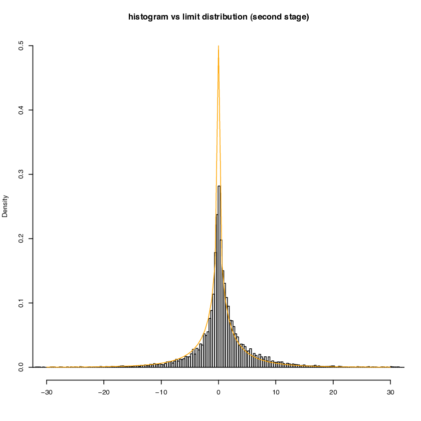
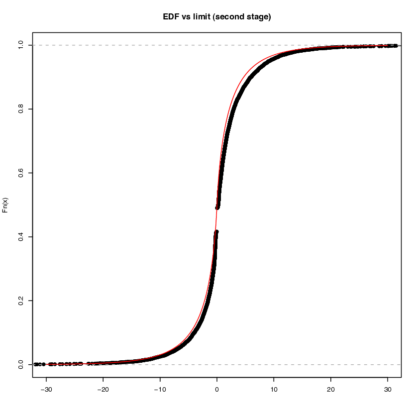
(see e.g. Csörgő and Horváth, 1997). In Figure 1 we report the graphical representation of the histogram and empirical distribution function of ZZ (over 10000 Monte Carlo replications) against their theoretical counterparts which looks quite reasonable.

nn ana_{n} t~n\tilde{t}_{n} θ^0\hat{\theta}_{0} θ^1\hat{\theta}_{1} t^n\hat{t}_{n} θˇ0\check{\theta}_{0} θˇ1\check{\theta}_{1} tˇn\check{t}_{n}
5000 0.1189 0.601 0.200 0.319 0.601 0.200 0.319 0.601
(0.005) (0.009) (0.014) (0.011) (0.005) (0.013) (0.012)
2000 0.1495 0.601 0.200 0.349 0.601 0.200 0.349 0.601
(0.008) (0.013) (0.020) (0.014) (0.008) (0.017) (0.015)
1000 0.1778 0.601 0.199 0.377 0.601 0.200 0.377 0.602
(0.011) (0.017) (0.025) (0.019) (0.011) (0.026) (0.018)
Table 1: Monte Carlo estimates for model (12) over 1000010000 replications. True values: θ0∗=0.2\theta_{0}^{*}=0.2, θ1∗=0.378\theta_{1}^{*}=0.378, 0.3500.350, and 0.3190.319 for different sample sizes n=1000n=1000, 20002000 and 50005000. True change point t∗=0.6t^{*}=0.6.
nn ana_{n} t~n\tilde{t}_{n} θ^0\hat{\theta}_{0} θ^1\hat{\theta}_{1} t^n\hat{t}_{n} θˇ0\check{\theta}_{0} θˇ1\check{\theta}_{1} tˇn\check{t}_{n}
5000 0.1189 0.701 0.200 0.319 0.701 0.200 0.319 0.701
(0.010) (0.012) (0.018) (0.011) (0.018) (0.012) (0.010)
2000 0.1495 0.702 0.200 0.350 0.701 0.200 0.350 0.701
(0.016) (0.016) (0.029) (0.024) (0.009) (0.030) (0.021)
1000 0.1778 0.703 0.200 0.378 0.701 0.200 0.377 0.701
(0.025) (0.021) (0.040) (0.038) (0.012) (0.056) (0.040)
Table 2: Monte Carlo estimates for model (13) over 1000010000 replications. True values: θ0∗=0.2\theta_{0}^{*}=0.2, θ1∗=0.378\theta_{1}^{*}=0.378, 0.3500.350, and 0.3190.319 for different sample sizes n=1000n=1000, 20002000 and 50005000. True change point t∗=0.7t^{*}=0.7.
Refer to caption
Refer to caption
Figure 1: Histogram versus theoretical density function (up) and empirical distribution function versus theoretical distribution function (bottom) for the second stage change point estimator. Results of 10000 Monte Carlo replications and sample size n=5000n=5000 for the first model.

References

  • [1] Bai, J. (1994) Least squares estimation of a shift in linear processes, Journal of Times Series Analysis, 15, 453-472.
  • [3] Bai, J. (1997) Estimation of a change point in multiple regression models, The Review of Economics and Statistics, 79, 551-563.
  • [5] Chen, G., Choi, Y.K., Zhou, Y. (2005) Nonparametric estimation of structural change points in volatility models for time series, Journal of Econometrics, 126, 79-144.
  • [7] Cox, J.C., Ingersoll, J.E., Ross, S.A. (1985) A theory of the term structure of interest rates, Econometrica, 53, 385–408.
  • [9] Csörgő, M., Horváth, L. (1997) Limit Theorems in Change-point Analysis. New York: Wiley.
  • [11] De Gregorio, A., Iacus, S.M. (2008) Least squares volatility change point estimation for partially observed diffusion processes, Communications in Statistics, Theory and Methods, 37(15), 2342-2357.
  • [13] Hinkley, D.V. (1971) Inference about the change-point from cumulative sum tests, Biometrika, 58, 509-523.
  • [15] Inclan, C., Tiao, G.C. (1994) Use of cumulative sums of squares for retrospective detection of change of variance, Journal of the American Statistical Association, 89, 913-923.
  • [17] Kim, S., Cho, S., Lee, S. (2000) On the cusum test for parameter changes in GARCH(1,1) models. Commun. Statist. Theory Methods, 29, 445-462.
  • [19] Kutoyants, Y. (1994) Identification of Dynamical Systems with Small Noise, Kluwer, Dordrecht.
  • [21] Kutoyants, Y. (2004) Statistical Inference for Ergodic Diffusion Processes, Springer-Verlag, London.
  • [23] Lee, S., Ha, J., Na, O., Na, S. (2003) The Cusum test for parameter change in time series models, Scandinavian Journal of Statistics, 30, 781-796.
  • [25] Lee, S., Nishiyama, Y., Yoshida, N. (2006) Test for parameter change in diffusion processes by cusum statistics based on one-step estimators, Ann. Inst. Statist. Mat., 58, 211-222.
  • [26] Shixin, G. (1997) The Hájek-Rényi inequality for Banach space valued martingales and the pp smoothness of Banach spaces, Statistics and Probability Letters, 32, 245-248.
  • [27] Song, J., Lee, S. (2009) Test for parameter change in discretely observed diffusion processes, forthcoming in Statistical Inference for Stochastic Processes.
  • [28] Woyczyński, W.A. (1975) Geometry and Martingales in Banach Spaces, in Winter School on Probability, Kapracz, Springer Lecture Notes in Mathematics, Vol. 472, 235-275
  • [29] Yoshida, N.: Polynomial type large deviation inequality and its applications. reprint (2005), to appear in Annals of the Institute of Statistical Mathematics