Topics in Heegaard Floer homology
Abstract.
Heegaard Floer homology is an extremely powerful invariant for closed oriented three-manifolds, introduced by Peter Ozsváth and Zoltán Szabó. This invariant was later generalized by them and independently by Jacob Rasmussen to an invariant for knots inside three-manifolds called knot Floer homology, which was later even further generalized to include the case of links. However the boundary maps in the Heegaard Floer chain complexes were defined by counting the number of points in certain moduli spaces, and there was no algorithm to compute the invariants in general.
The primary aim of this thesis is to address this concern. We begin by surveying various areas of this theory and providing the background material to familiarize the reader with the Heegaard Floer homology world. We then describe the algorithm which was discovered by Jiajun Wang and me, that computes the hat version of the three-manifold invariant with coefficients in . For the remainder of the thesis, we concentrate on the case of knots and links inside the three-sphere. Based on a grid diagram for a knot and following a paper by Ciprian Manolescu, Peter Ozsváth and me, we give a another algorithm for computing the knot Floer homology. We conclude by generalizing the construction to a theory of knot Floer homotopy.
1991 Mathematics Subject Classification
57M27Acknowledgement
My adviser Zoltán Szabó for introducing me to the fascinating world of Heegaard Floer homology and for guiding me throughout the entire course of my graduate studies.
My collaborators Matthew Hedden, András Juhász, Ciprian Manolescu, Peter Ozsváth and Jiajun Wang for all the discoveries that we made together, which constitute a significant portion of this thesis.
The FPO committee members William Browder, David Gabai and Zoltán Szabó and the thesis readers Peter Ozsváth and Zoltán Szabó.
Boris Bukh, William Cavendish, David Gabai, Matthew Hedden, András Juhász, Robert Lipshitz, Ciprian Manolescu, Peter Ozsváth, Jacob Rasmussen, Sarah Rasmussen, Zoltán Szabó and Dylan Thurston for many enjoyable conversations and lots of interesting remarks.
The Fine Hall common room for providing the perfect ambience to do Mathematics.
My parents, my brother and my sister for everything.
Thank you.
Chapter 1 Beginning of days
Our story starts on a summer day in , when two Hungarian mathematicians sat together for a few hours, and came up with one of the most amazing theories in modern low dimensional topology.
1.1. Low dimensional topology
Low dimensional topology is the branch of differential topology that deals with three-dimensional and four-dimensional manifolds. It seems strange at first to concentrate on just these two dimensions, when there are (countably) infinite number of other dimensions we could have worked with. The justification of this restricted choice lies in Smale’s h-cobordism theorem. When stated in simple (and incorrect) terms, it basically says that in high enough dimensions, homotopy restrictions give information about smooth structures, and hence differential topology follows from algebraic topology. Stated in a more mathematical form, it says
Theorem 1.1.1.
[Sma62] If and is a cobordism between two simply connected manifolds and , and each of the inclusions induces a homotopy equivalence, then is diffeomorphic to .
The condition that is very crucial in the statement, and appears in a very subtle way in the proof. The fact that it is necessary was established by Donaldson, when he disproved the h-cobordism statement for . The status of the statement in other smaller dimensions may be of independent interest. For , it is trivial and for it is vacuous. The case was proved recently by Perelman during his proof of the Poincaré conjecture. The case stays unconquered (and as a consequence of Perelman’s work, is now equivalent to the smooth four-dimensional Poincaré conjecture).
As mentioned at the beginning of this section, this leaves the story in dimensions three and four wide open. From the void of uncertainty to the pristine beauty of an unexplored world, sprang forth low dimensional topology.
1.2. Knot Theory
One of the greatest treasures in the galleries of low dimensional topology is the fascinating world of knots. To appreciate fully the wonders of this new world, we need to familiarize ourselves with a few basic definitions first. However to avoid pathologies, we always work in either the smooth category or the piecewise-linear category, and to remain intentionally vague, we mention this fact only once and never allude to it again.
Definition 1.2.1.
A knot is an embedding of the circle into the three-sphere . Two knots and are said to be equivalent if there is an isotopy of (i.e. an one-parameter family of diffeomorphisms of to itself) that takes to .
Definition 1.2.2.
A knot diagram is an immersion of the circle into the two-plane , such that there are no triple points, and at every double point one of the participating arcs is declared the overpass (the other one the underpass).
Knot theory started long before low dimensional topology came into fashion. Historically knots were always described by knot diagrams. Given a knot diagram, it is easy to recover a knot from it, by embedding into in a standard way, and then obtaining an embedded in from the immersed in using the crossing information, and finally one-point compactifying to get . It is not difficult to see that given a knot, there is always a knot diagram representing it. Figure 1.1 shows a knot diagram representing a right-handed trefoil knot.

However it is always the case with these sorts of knot presentations that while such a presentation exists, it is far from canonical. In other words, even though every knot can be represented by a knot diagram, two different knot diagrams can correspond to the same knot. (Here, by two different knot diagrams, we mean two knot diagrams that cannot be related by an isotopy of .) Figure 1.2 illustrates two such knot diagrams, either of which represents the trivial knot, or the unknot.

In 1927, Alexander and Briggs, and independently Reidemeister came up with essentially three local moves on knot diagrams, such that two knot diagrams represent the same knot if and only if one can be taken to the other using only these moves.
Theorem 1.2.3.

One of the central problems in knot theory is distinguishing two knots. In other words, given two knot diagrams, we want to know whether or not they represent the same knot. In case they do, it is usually very easy to show that they do, simply by relating one knot diagram to another using Reidemeister moves (however easy is relative, see for example Figure 1.2). In case they do not, i.e. the two knot diagrams represent different knots, they are usually shown to be different using some invariants.
The first and the most classical invariant (and also the most non-maneuverable one) is the fundamental group of the knot complement, more commonly known as the knot group. The knot group is already enough to distinguish the unknot from the trefoil (in fact it is a theorem that the knot group distinguishes the unknot, but it is not always easy to check whether or not two groups are isomorphic). The knot group of the unknot is , and a clever application of Van Kampen shows that the knot group of the trefoil is given by the group presentation , which has a very natural surjection to , the symmetric group on three letters.
However most of the other classical invariants of knots are defined as invariants of knot diagrams, which are then shown to remain invariant under the Reidemeister moves. Perhaps the most famous knot invariant of all times, the Alexander polynomial, can be argued to belong to this category. In the original definition by J.W.Alexander [Ale28] where it is defined as the generator of a principal ideal domain over , the polynomial is only defined up to a multiplication by . John Conway later showed that the polynomial satisfies a linear Skein relation, and its value on the unknot was enough to determine it, and a reparametrized version of the Alexander polynomial is called the Alexander-Conway polynomial. Throughout this thesis, we will be referring to the normalized but unparametrized version of the polynomial as the Alexander polynomial (even though technically it is a Laurent polynomial). For example, the Alexander polynomial for the unknot is and the Alexander polynomial for the trefoil is .
Much later Kauffman presented a combinatorial description of the Alexander polynomial without using Skein relation, and defined only in terms of a knot diagram. Given a knot diagram, let regions be the connected components of the complement of the immersed circle in . Let be the unbounded region, and let be another region adjacent to the unbounded region.
Definition 1.2.4.
[Kau83] A Kauffman state is a map which assigns to each double point of the knot diagram, a region adjacent to it, such that each region other than and is assigned to some double point.
Let us now work with oriented knots, represented by oriented knot diagrams. Given a Kauffman state and a double point , let be defined according to Figure 1.4.

Theorem 1.2.5.
[Kau83] For a knot presented in an oriented knot diagram, let be the set of all Kauffman states and let be the set of all double points. Then the Alexander polynomial of the knot is given by .
The other central problem in knot theory is understanding geometric properties of knots. This is the area where there is the closest interaction between knot theory and other aspects of low dimensional topology. It can be argued that understanding three-manifolds is equivalent to understanding knots inside the three sphere . To state precise mathematical results in support of this claim, we first need to extend the world of knots to embrace links.
Definition 1.2.6.
A link is an embedding of a disjoint union of circles into . Two links are said to be equivalent if there is an isotopy of that takes one link to another. Each circle in the link is called a link component.
Planar link diagrams are defined similarly, and once more two link diagrams represent the same link if and only if they can be connected by a sequence of Reidemeister moves. The following theorem by Alexander is the first indication of how links are related to three-manifolds.
Theorem 1.2.7.
[Ale20] Any oriented three-manifold is branched cover of with the branch set being a link.
However there is an even more subtle relation between links in and three-manifolds. A surgery on a link is a procedure by which we remove a tubular neighborhood of a link in and then glue back the neighborhood (which is a disjoint union of solid tori) in a (possibly) different fashion. It is an amazing theorem that,
Theorem 1.2.8.
Every oriented three-manifold is a surgery along some link in .
It is not surprising then that many geometric properties of knots and links translate to properties of three-manifolds. We end this section after discussing the geometric property that concerns us the most, the Seifert genus of a knot.
Definition 1.2.9.
A Seifert surface for a knot is a compact oriented surface embedded in such that .
Seifert showed [Sei35] that every knot admits a Seifert surface, thus leading to the definition of the Seifert genus of a knot.
Definition 1.2.10.
The genus of a knot is the smallest number among the genera of the Seifert surfaces that bound .
It is easy to see that the unknot is the only knot of genus . Figure 1.5 shows a genus one surface bounding the right-handed trefoil, thus showing that the trefoil has genus .

From the very nature of the definition of the genus of a knot, it is obvious that it is a knot invariant, but a priori it is not even clear whether or not it can be computed. Amazingly the Alexander polynomial provides some information about the genus.
Theorem 1.2.11.
The normalized Alexander polynomial is a symmetric Laurent polynomial, and the genus of a knot is at least the degree of its Alexander polynomial.
For example, the Alexander polynomial for the -torus knot is , which shows that the genus of the -torus knot is at least three. (The genus is in fact equal to three, as seen by cleverly finding a genus three Seifert surface).
Before we conclude this section, we should mention that this section has been a mere glimpse at the wonderful world of knots and links. We have only talked of theorems which have some (often minor) connections with the rest of the thesis, and left hundreds of other stories in knot theory untold.
1.3. Floer homology
We take leave of low dimensional topology to take a brief detour to the realms of Floer homology. Historically, Floer homology deals with two -dimensional Lagrangians inside a -dimensional symplectic manifold. However we will be dealing with a slightly different situation. What follows is one of the simplest versions of Floer homology, suited to our specific needs.
Let be a closed manifold with a complex structure. Let the induced almost complex structure be , i.e. is a map from the tangent bundle to itself with . A totally real subspace is a submanifold such that if is a non-zero tangent vector to , then is not a tangent vector to . Clearly the dimension of a totally real subspace it at most . Let and be two totally real subspaces which are transverse to one another. Thus and intersect in a finite number of points.
Let us work over a commutative ring (usually it is or ). The chain complex is the free -module generated by the finitely many points in . Given , a Whitney disk joining to is a map from the unit disk in the complex plane to such that , , and . Two such Whitney disks are said to be homotopic to one another, if they are homotopic relative the boundary conditions. Let be the set of all Whitney disks joining to up to homotopy equivalence. Note that given a Whitney disk joining to and another Whitney disk joining to , we can glue them together to get a Whitney disk joining to . This gives a natural map (which we denote by ) from to which we will need later.
To define the Floer homology we need a chain complex. We already have the generators for the chain complex, namely the points in , so all that we need are the boundary maps. This is where things get complicated. The boundary map depends on a function called the count function, which maps Whitney disks to , and for , can be written as
This definition immediately leads to further questions. It is not even clear a priori that given , there are finitely many . Thus for the definition to even make sense, we must have for all but finitely many .
The second and more important issue is that there is no guarantee that . The definition of the count function has to be specially designed to ensure this. The usual way to define is the following.
We first choose a number of divisors (complex submanifolds, each with real dimension ) each disjoint from . The chain homotopy type of the Floer chain complex would very much depend on the choice of these divisors. Then given a Whitney disk , its algebraic intersection number with each of the ’s is well-defined, since the boundary of the Whitney disk lies on and ’s are disjoint from . We declare if for some .
Given a Whitney disk , let its moduli space be the space of all complex maps from the unit disk in to which represent . Let the Maslov index be the expected dimension of the moduli space. We once more declare if .
There is a natural action of on given by the precomposition by the one-parameter family of diffeomorphisms of which fixes and . Let be the reparametrized moduli space. If , the expected dimension of is one, and hence the expected dimension of is zero. Let us assume that the complex structure on is generic enough such that whenever , the actual dimension of is zero, and it consists of finitely many points. There is usually an orientation on which induces a sign of on these points, and the aptly named count function is simply the count of these points with sign. Since we are still in complete awe of the definition of the Floer chain complex, let us restate it once more in the light of new knowledge.
The reason for introducing the divisors ’s in the definition is two fold. Usually if there are enough divisors, then given , all but finitely many of will not be disjoint from , and hence will be zero for all but finitely many .
The second reason is slightly more subtle. Recall that we also need to be a boundary map, i.e. . What this translates to is the following. For all ,
We may in addition assume that both and are disjoint from the divisors, and either has . Since the Maslov index is additive, this would imply is a Whitney disk of Maslov index two. Thus given and a Whitney disk with which avoids all the divisors, it is enough to show that,
It is clear that to understand , we need to understand . Recall that for a Whitney disk , the expected dimension of is . So assume that the complex structure on is generic enough, such that for all Whitney disks with , it is a collection of finitely many points when , and it a compact one-manifold when .
Let us now analyze the boundary degenerations of . The Maslov indices of the different components in a boundary degeneration has to add up to , and the index of each component has to be at least one, so there has to be exactly two components in each boundary degeneration. Thus only three types of boundary degenerations as shown in Figure 1.6, are possible.

Somehow by a miracle, if there are enough divisors such that every holomorphic Maslov index one Whitney disk whose boundary lies entirely in one of and , intersects one of ’s, then the Cases and of Figure 1.6 cannot occur. Then the sum counts precisely the number of boundary points of (with orientation). However since is a compact one-manifold, it has an even number of boundary points, and hence the sum (even with sign) is zero, leading to a proof that .
1.4. Heegaard Floer homology
Heegaard Floer homology is an amazing application of the techniques of Floer homology where all these miracles do indeed come true. It was introduced in a couple of revolutionary papers [OS04d, OS04c] by Peter Ozsváth and Zoltán Szabó, primarily as an invariant for closed three-manifolds. From now on, assume all the three-manifolds are closed, connected and oriented.
Definition 1.4.1.
A genus Heegaard splitting of a three-manifold is a decomposition of into a union of two oriented genus handlebodies and , which are glued together by an orientation reversing diffeomorphism .
It is clear that given two handlebodies and a gluing map between them, we get a three-manifold. It is perhaps not that clear that every three-manifold admits a Heegaard decomposition. However it is a well known theorem that,
Theorem 1.4.2.
Every oriented three-manifold admits a Heegaard decomposition.
One way to see this is by constructing Morse function on the three-manifold .
Definition 1.4.3.
A Morse function on a manifold is a smooth function , such that at every critical point (i.e. where ), the Hessian is non-singular. The index of a critical point is the number of negative eigenvalues of the Hessian. A Morse function is said to be self-indexing if at every critical point the value of the Morse function equals the index of the critical point.
Definition 1.4.4.
A gradient-like flow associated to a Morse function on is a flow whose singularities are precisely the Morse critical points, and furthermore the flow agrees with a gradient flow induced from some metric in a neighborhood of the critical points, and the Morse function is a strictly decreasing function along any flowline.
It is an extremely important result that every oriented smooth manifold admits a self-indexing Morse function and a gradient-like flow associated to it. In fact given a natural number , we can even ensure that the Morse function has exactly maxima and minima. Thus to find a Heegaard decomposition of a three-manifold , all we need to do is to find a self-indexing Morse function , and then define the handlebodies and as and respectively.
We choose the Morse function to have exactly maxima and minima (usually we choose ). This implies (since ) that the number of index critical points must equal the number of index critical points. Let the common number be . Then is a genus surface and the Heegaard decomposition described in the previous paragraph is a genus Heegaard decomposition.
In addition, if we are given a gradient like flow associated to this Morse function, then we can represent the whole picture by a single combinatorial diagram on the Heegaard surface . Let (numbered arbitrarily) be the disjoint circles on that flow down to the index one critical points, and let (also numbered arbitrarily) be the circles that flow up to the index two critical points. While choosing the gradient-like flow, we ensure that the circles intersect the circles transversely. Clearly the circles are disjoint from one another, and their complement has components flowing down to the index zero critical points, and thus the circles generate a half-dimensional subspace of . A similar statement holds for the circles. We also choose basepoints (needless to say, also numbered arbitrarily) such that each component of contains one basepoint, and each component of contains one basepoint. Such a diagram is called a Heegaard diagram, but for future convenience, let us record the definition here.
Definition 1.4.5.
A Heegaard diagram is genus- surface with two collections of disjoint curves, called curves and curves respectively, and basepoints such that has components each with a basepoint, and also has components each containing a basepoint.
It is reasonably clear that a Heegaard diagram captures all the information that is needed to reconstruct the three-manifold . We thicken to get . We add two-handles to and to . This results in a three-manifold with boundary components each homeomorphic to . We add solid balls to each boundary component to recover the three-manifold . Figure 1.7 shows a genus-two Heegaard diagram (with ) representing .

Thus every Heegaard diagram represents a specific three-manifold, and any three-manifold can be represented by a Heegaard diagram. However there can be lots of Heegaard diagrams representing the same three-manifold. It turns out that any two Heegaard diagrams representing the same three-manifold can be related by a sequence of moves of the following type.
Definition 1.4.6.
In an isotopy, the and the curves move independently (i.e. it does not have to be induced from an isotopy on the whole surface) by isotopies in the complement of the basepoints.
Definition 1.4.7.
In a handleslide of the curves, we take a pair of pants region bounded by the curves , and which does not contain any basepoint, and whose intersection with the curves is precisely the union of the circles and , and we then replace the curve with a new curve . A handleslide of the curves is defined similarly.
Definition 1.4.8.
In a stabilization of the first type, we increase the genus of the Heegaard surface by adding an one-handle, and we add an curve and a curve as shown in Figure 1.8. A destabilization of the first type is the reverse of this move.
Definition 1.4.9.
In a stabilization of the second type, we add one circle, one circle and one basepoint like in 1.8. A destabilization of the second type is the reverse of this move.
The moves (other than isotopy) are shown in Figure 1.8. It is clear that these moves do not change the underlying three-manifold. Interestingly, the following theorem shows that some sort of a converse is also true.

Theorem 1.4.10.
Two Heegaard diagrams represent the same three-manifold if and only if they are related by a sequence of isotopies, handleslides, and stabilizations and destabilizations of either type. In fact two Heegaard diagrams with the same number of basepoints representing the same manifold can be related by a sequence of isotopies, handleslides and stabilizations and destabilizations of the first type only.
Now, given a three-manifold , we (essentially by choosing a specific type of Morse function, and a gradient like flow corresponding to it) choose a Heegaard diagram representing . Consider the symmetric product , where is the group of permutations on letters acting naturally on the Cartesian product. Even though the action of on the Cartesian product is far from a free action, the quotient turns out to be manifold (this follows from the observation , a consequence of the fundamental theorem of algebra). We choose a complex structure on , which in turn induces a complex structure on , and a generic perturbation (in a precise sense, as described in [OS04d]) of this complex structure is chosen. We are soon going to apply the heavy machinery of Floer theory, and this dimensional manifold is the complex manifold that we start with.
Given any permutation , there is a dimensional torus in . These tori are all disjoint (this is just an extremely fancy way of saying that the circles are disjoint), and the action of simply permutes these tori. Thus , the quotient of these tori, lying in (and denoted by ) is also a torus, and is a half-dimensional totally real subspace. The torus is defined similarly.
We are almost set for applying the Floer machinery. We have the -dimensional complex manifold, and two totally real -dimensional subspaces. The divisors are all that we need. Recall that the symmetric product is just the parametrizing space of unordered -tuples of points on the surface. Let be the codimension-two holomorphic subspace consisting of all the points in the symmetric product whose one of the coordinates is the basepoint . Once more, the statement that is disjoint from is a fancy restatement of the fact that lies in the complement of the and curves.
Now finally, at the end of the beginning, we define the Floer chain complex. The chain complex is the free -module generated by , and for a generator , the boundary map is given by
The chain complex defined above is called the hat version of the Heegaard Floer chain complex (hence the notation ). In order to complete our eduction, there is another important chain complex that we need to know of, called the minus version of the Heegaard Floer chain complex. The new chain complex is the -module generated freely by points of , and the boundary map is defined on each generator as follows
We have made lots of choices on the way. We have chosen a self-indexing Morse function with maxima and minima, we have chosen a gradient-like flow corresponding to it, we have chosen basepoints (subject to certain restrictions), we have chosen a complex structure on the Heegaard surface and a generic perturbation of the induced complex structure on the symmetric product, and finally we have chosen a ring which is usually or . If the three-manifold is a rational homology sphere, i.e. if , then this is all we need. If however , then for the hat version, we also need to ensure that the Heegaard diagram is admissible, and for the minus version, we need to ensure that the diagram is strongly admissible. These are minor technical restriction that we do not need to bother ourselves with.
We end this section with the following wonderful theorems, established by Ozsváth and Szabó, which can easily be named the Fundamental Theorems of Heegaard Floer Homology. The theorems basically say that the homologies of the chain complexes are three-manifold invariants.
Theorem 1.4.11.
[OS04d] The map defined above is a boundary map, i.e. , and there is an -module depending only on and , such that the homology of the hat version of the Floer chain complex is isomorphic to .
Theorem 1.4.12.
[OS04d] The map defined above is also a boundary map, and there is an -module depending only on and , such that the homology of the minus version of the Floer chain complex is isomorphic to as -modules, where the action on the Floer homology is given by multiplication by any of the ’s.
1.5. Knot Floer homology
The last time we talked about knots, we only talked about knots and links inside the three-sphere . This is because for the most part in this thesis, we will not be needing the general case. However, in general, a link is an embedding of a disjoint union of circles inside a three-manifold , and a knot is a link with one component. The following is a Heegaard diagram describing a link.
Definition 1.5.1.
A link Heegaard diagram is genus- surface with two collections of disjoint curves, called curves and curves respectively, and two collections of basepoints called points and points respectively, such that has components each with a -basepoint and a -basepoint, and also has components each containing a -basepoint and -basepoint.
Given a link Heegaard diagram, observe that if we forget about the -basepoints, we get an ordinary Heegaard diagram. The three-manifold which that Heegaard diagram represents is the ambient three-manifold . To recover the link , in each component of join to by an embedded oriented arc avoiding all the curves, and then push the interior of this arc towards the -handlebody (i.e. the handlebody in which all the curves bound disks). Similarly in each component of join to by an embedded oriented arc avoiding all the curves, and then push the interior of the arc towards the -handlebody . The resulting one-dimensional oriented subspace of is the link .
More often than not, we work with knots inside . In that case, we usually choose , although for the most part in this thesis, we will not be doing that. Figure 1.9 shows a Heegaard diagram for the trefoil inside with .

Knot Floer homology was introduced by Peter Ozsváth and Zoltán Szabó [OS04b] and independently by Jacob Rasmussen in his PhD thesis [Ras03]. It was later generalized by Ozsváth and Szabó to include the case of links [OS08], but for now, let us just present the definition of knot Floer homology.
Given an oriented knot inside an oriented three-manifold , let be an admissible Heegaard diagram representing the knot. It turns out that there is always such a Heegaard diagram, and two such Heegaard diagrams with the same number of basepoints are related by a sequence of isotopies, handleslides and stabilizations and destabilizations of the first type in the complement of both the -basepoints and the -basepoints. We once more choose a complex structure on and then take a generic perturbation of the induced complex structure on . Let and be the two totally real half-dimensional tori, and let and be the codimension-two holomorphic subspaces. Fix a commutative ring (once more, usually or ). For the hat version, the chain complex is the -module freely generated by , and for a generator , the boundary map is given by
In the minus version, the chain complex is the -module freely generated by , and for a generator , the boundary map is given by
The natural analogues of Theorems 1.4.11 and 1.4.12 hold, and thus in both the hat version and the minus version, Heegaard Floer homology presents us with knot invariants called knot Floer homology and denoted by and . However in certain cases, especially for knots inside , the invariant has more structure than meets the eye, and hence from now on until the end of this section, let us always choose the ambient three-manifold to be .
Given two generators , the space of Whitney disks joining them , is isomorphic to for (a minor restriction that can easily be ensured by stabilization). In fact, in the next section, we will introduce a slightly different definition of and under the new definition, the space of Whitney disks joining any two points will always be isomorphic to for integral homology spheres. Choose a Whitney disk . For any point , let (we are mostly interested in the case when is one of the basepoints). Then define the relative Maslov grading to be and the relative Alexander grading to be . It is relative easy to check that the definition is independent of the choice of , and the only subtlety in showing that they are indeed relative gradings (i.e. and ) lies in the observation that the Maslov index is additive.
The definitions convert the hat version of the chain complex to a relatively bigraded -module (we declare all elements of to have bigrading ). The minus version of the chain complex can also be made a relatively bigraded -module by declaring each to have bigrading . It is easy to check that in both the hat and the minus version, the boundary map reduces the Maslov grading by one and keeps the Alexander grading constant. Thus in either case, the homology carries a relative bigrading, where the relative Maslov grading is essentially the homological grading. This induces a relative bigrading on and . For the hat version, in each copy of , the two generators are declared to have -bigradings of and , and thus we get an induced bigrading on too. Further note that the definition of the relative Maslov grading did not use the -basepoints, and hence the relative Maslov grading is in fact a relative grading on the Heegaard Floer homology of the ambient three-manifold.
The three-sphere admits a Heegaard diagram with only one generator (in fact it is the only three-manifold to admit such Heegaard diagrams) and hence . For knots inside , the relative Maslov grading can be lifted to an absolute Maslov grading (also denoted by ) by declaring the absolute Maslov grading of the generator of to be zero. There is a similar well-defined lift of the relative Alexander grading to an absolute one. It is defined to be the unique lift such that following property holds.
The not so obvious fact that there is such a lift, and it is unique, is a simple consequence of the following cute theorem by Ozsváth and Szabó. The proof uses Kauffman’s definition of Alexander’s polynomial, and we leave it as something for the interested reader to prove or look up.
Theorem 1.5.2.
[OS04b] The Alexander polynomial is the Euler characteristic of the knot Floer homology, or in other words the Alexander polynomial of a knot is equal to , where is the part of the hat version of knot Floer homology in bigrading .
Recall that the Alexander polynomial provided some information about the genus of a knot. It is only natural to expect that the knot Floer homology will also provide some information about the genus. However it turns out that, due to yet another amazing theorem by Ozsváth and Szabó, the knot Floer homology in fact determines the genus.
Theorem 1.5.3.
[OS04a] If is the genus of a knot , then is the highest Alexander grading such that is non-trivial (with coefficients in ).
Thus, modulo an algorithm to calculate the knot Floer homology, the above theorem provides a way to calculate a geometric invariant, the genus of a knot. Another geometric property of knots that can be computed using knot Floer homology is fiberedness. A knot is said to be fibered if the knot complement is a fiber bundle fibering over the meridian (a meridian is a simple closed curve on the boundary of a tubular neighborhood of the knot, which bounds a disk inside the neighborhood). The strength of knot Floer homology as a knot invariant is further established by the following theorem proved by Yi Ni [Ni07] and later by András Juhász [Juh08].
1.6. Cylindrical Reformulation
The story of Floer homology that we have described so far involves maps from a disk to high dimensional complex manifolds. Not only are such maps incredibly hard to maneuver, they are also incredibly hard to visualize. In a remarkable paper [Lip06], Robert Lipshitz presented the cylindrical reformulation of Heegaard Floer homology, which made certain aspects somewhat unnatural, but made almost all the aspects easier to compute, and as a side product produced a combinatorial formula for the Maslov index.
Let us restrict ourselves to the case of closed three-manifolds since the case for knots inside three-manifolds is very similar. Let be an admissible Heegaard diagram for a three-manifold . A generator is a formal sum of distinct points on such that each circle contains one point and each circle contains one point. (It is easy to see that generators correspond to points of .) Let be the set of all such generators. A domain joining to is a -chain generated by components of such that , and by a (slight) misuse of notation, the set of all domains joining to is denoted by . It is not true that domains joining to correspond to Whitney disks joining to in the symmetric product, but however given a Whitney disk , there is a domain associated to it, defined as follows. A region is defined to be a component of and the coefficient of the -chain at a region is defined to be where is any point in the region. In fact for , this association is bijective.
If is a point of intersection between an and a curve, and is some -chain generated by regions, then is defined to be the average of the coefficients of at the four (possibly different) regions around . Then for a generator , the point measure is defined as .
Fix a metric on the surface such that all the curves and all the curves are geodesics and they intersect each other at right angles. For any -chain generated by the regions, define the Euler measure as times the integral of the curvature along the -chain . Being an integral, the Euler measure is additive, which implies that if where ’s are integers and ’s are regions, then . Also note that if a region is a -gon (i.e. if it is homeomorphic to an open ball, and if it has arcs and arcs on its boundary), then .
Given a domain (and after another minor abuse of notation), the Maslov index is defined by the Lipshitz’ formula as . The abuse of notation is quickly justified by the following theorem by Lipshitz,
Theorem 1.6.1.
[Lip06] Let be a Whitney disk joining to in the symmetric product, and let be domain associated to it. Then .
The relative Maslov grading is defined similarly. If is an integer homology sphere, then for two generators and , choose , and define . This definition is again easily seen to be independent of the choice of the domain . However showing that this defines a relative grading, i.e. without resorting to the previous theorem involves more work, and is hereby left as a challenging exercise to the interested reader, see [Sar].
As before, if , then we require the Heegaard diagram to be admissible. This time, we will actually state precisely what this means. Let be the subset of consisting of all the domains with for all basepoints . A domain is called a periodic domain. For a diagram to be (weakly) admissible, we require all non-trivial periodic domains to have both positive and negative coefficients (as -chains).
Let us choose a complex structure on , and consider the induced complex structure on . In theory, we should be working with a generic perturbation of the complex structure, but that is where things get complicated, so for now, let us just stick to the induced complex structure. Let us consider a Whitney disk which has a holomorphic representative, i.e. can be thought of as a holomorphic map from the unit disk to the symmetric product, satisfying certain boundary conditions. There is a -sheeted holomorphic branched covering map . Therefore there is a compact surface (with boundary) which is -sheeted covering of the unit disk and a map such that the following diagram commutes.
We postcompose the map from to with the projection map to the first factor. Thus we get holomorphic maps from to and , and hence an induced holomorphic map (where the target has the product complex structure). Let and be the first projection and the second projection respectively, which implies that the map from to is and the -sheeted branched cover of over is . It is easy to see that the image of (as -chains) is , the domain associated to .
Let be the fat diagonal, i.e. the set of all unordered -tuples of points in where some two points are equal. It is a codimension-two holomorphic subspace which is disjoint from the two tori and . Thus for any Whitney disk , the intersection number is well-defined. The following relation was proved by Rasmussen in his PhD thesis,
Theorem 1.6.2.
[Ras03] For any Whitney disk , .
In light of Lipshitz’ formula, the above simplifies to give . Also note that the -sheeted branched cover of is branched precisely over the fat diagonal . Hence is branched over the unit disk precisely at the points which map by to . Hence the number of branch points of is .
The above observation also has the following two important implications. Firstly, all the branch points of lie in the interior of the disk , since the boundary of the disk maps to which is disjoint from the fat diagonal . This implies that the map is -sheeted covering map to the circle . Let be the preimages of and let be the preimages of (all numbered arbitrarily). The complement of the -points and -points in can be divided into arcs of two types -type and -type, where the -type arcs cover and -type arcs cover . Then on , the -points and the -points alternate, and the -type arcs and the -type arcs alternate. The boundary conditions on induce certain boundary conditions on , whereby the formal sum of the images of the -points is the generator , the formal sum of the images of the -points is the generator , the -type arcs map to the curves and the -type arcs maps to the curves.
Secondly, the holomorphic map is an embedding. For otherwise, if two distinct points and map to the same point , then is a -unordered tuple of points where two of the points are , and hence intersects the fat diagonal , and hence the map should have been branched over , implying .
All this says is that given a Whitney disk with holomorphic representatives, we can construct a Riemann surface (with boundary) and a holomorphic embedding , satisfying certain boundary conditions. Conversely, given a holomorphic embedding satisfying the previously mentioned boundary conditions, we can recover the Whitney disk . Since is a -sheeted branched cover, for each point , look at its -preimages in (possibly with multiplicities), and then map them by to get an unordered -tuple of points in or in other words a point in . This (holomorphic) map is the required Whitney disk .
The setting for the cylindrical reformulation of Floer homology is now clear. For some commutative ring , the hat version of the chain complex is the -module freely generated by . Given a domain joining a generator to a generator , the moduli space is the moduli space of all embeddings of compact Riemann surfaces , satisfying the above-mentioned boundary conditions such that the image of is . Here the complex structure on is a generic perturbation of the product complex structure, but throughout this section, we will keep things simple and assume that it is in fact the product complex structure. There is a natural -action on this moduli space given by postcomposing the map by the one-parameter family of diffeomorphisms of , and let the quotient be the reparametrized moduli space . It turns out that the expected dimension of is (and hence the expected dimension of is ), and for a generator , the hat version of the boundary map is given by
In the minus version, we are allowed to pass through the basepoints. The chain complex is the -module freely generated by , and for a generator , the boundary map is given by
We have spent a long time without any figures, so this is an opportune moment to introduce Figure 1.10, a genus two Heegaard diagram for with one basepoint. The genus two surface is obtained by gluing the circles that lie in the same horizontal level (which are also the circles), in an orientation reversing way such that the black dots on the circles match up. The shaded region is a (positive) Maslov index one domain joining the generator marked with white squares to the generator marked with white dots. Here is yet another tricky exercise for the curious reader. Show that (with the product complex structure on and coefficients in ) .

The following theorems bring relief, and justify the inclusion of the word ‘reformulation’ in the nomenclature of this section.
Theorem 1.6.3.
[Lip06] The homology of the hat version of the chain complex defined above is isomorphic to .
Theorem 1.6.4.
[Lip06] The homology of the minus version of the chain complex defined above is isomorphic to as -modules.
Before we conclude this section, we should mention the following few formulae, all of which are corollaries of the cylindrical reformulation.
Theorem 1.6.5.
[Lip06] The Euler characteristic of the surface is given by .
A component of the surface is called a trivial disk if it is a disk with only one -marking and one -marking on its boundary, and it maps to a single point in by . If is the image a trivial disk, then clearly is both an -coordinate and a -coordinate, and furthermore . Recall that the number of branch points of is . The number of branch points of can also be computed as where is the number of trivial disks.
There is one last thread that we need to wrap up. It is a simple observation, but an extremely important one.
Theorem 1.6.6.
If , then is a positive domain, i.e. for all points .
Proof.
If , then there is a holomorphic map representing the domain . However is the intersection between and , and assuming the complex structure is the product complex structure (at least in a neighborhood of ), both the subspaces are holomorphic objects and hence they intersect non-negatively, thus concluding the proof. ∎
Chapter 2 Letting bigons be bigons
Heegaard Floer homology is a great invariant. Other than being completely new and extremely powerful, it also enjoys a geometric lineage which allows it to provide information about many geometric properties of three-manifolds. (One prime example of this phenomenon is knot Floer homology for knots in determining the knot genus.) Hopefully our brief encounter with Heegaard Floer homology in the previous chapter has already convinced the reader of this fact.
However there is one minor inconvenience in the whole theory. Till date, it has not admitted any combinatorial reformulation. For example, there is no algorithm to compute for any ring (just a word caution, we are not claiming whether or not there can be any algorithm, it is just that until now we have not discovered any). In this chapter we present a partial solution to the problem, mostly following the lines of the paper [SW] by Jiajun Wang and the present author.
2.1. Consequences of being nice
We restrict our attention to some special Heegaard diagrams called nice pointed Heegaard diagrams. The terminology is perhaps a little unfortunate, since the term ‘nice’ is neither mathematical, nor an accurate description of these types of Heegaard diagrams.
Definition 2.1.1.
Let be a Heegaard diagram for a three-manifold . The diagram is called a nice pointed diagram if any region that does not contain any basepoint is either a bigon or a square.
Let be a closed oriented three-manifold. Suppose has a nice admissible Heegaard diagram (in fact it is not so hard to see that a diagram being nice implies that the diagram is admissible, see [LMW]). We choose a product complex structure on .
Definition 2.1.2.
A domain with coefficients and is called an empty embedded -gon, if it is topologically an embedded disk with vertices (a vertex being a point of the form or ) on its boundary, such that at each vertex , , and it does not contain any or in its interior.
The following theorems show that, for a domain (or in other words, a domain which avoids all the basepoints, i.e. for all ), the count function if and only if is an empty embedded bigon or an empty embedded square, and in that case . Thus can be computed combinatorially in a nice Heegaard diagram.
Theorem 2.1.3.
[SW] Let be a domain such that . If has a holomorphic representative, then is an empty embedded bigon or an empty embedded square.
Proof.
We know that only positive domains can have holomorphic representatives. We also know that bigons and squares have non-negative Euler measure. We will use these facts to limit the number of possible cases.
Suppose , where ’s are regions (i.e. components of ) containing no basepoints. Since has a holomorphic representative, we have , for all . Since each is a bigon or a square, we have and hence . So, by Lipshitz’ formula , we get .
Now let and , with . We say hits some circle if is non-zero on some part of that circle. Since , it has to hit at least one circle, say , and hence as . Also if does not hit , then and they must lie outside the domain , since otherwise we have and hence becomes too large.
We now note that can only take half-integral values, and thus only the following cases might occur.
- •
hits and another circle, say , consists of squares, , and there are trivial disks.
- •
hits , consists of squares and exactly one bigon, , and there are trivial disks.
- •
hits , consists of squares, , and there are trivial disks.
Using the reformulation by Lipshitz, in each of these cases, we will try to figure out the surface which maps to . Recall that a trivial disk is a component of which maps to a point in after post-composing with the projection .
The first case corresponds to a map from to with , and has trivial disk components. If the rest of is , then is a double branched cover over with one branch point and with , i.e. is a disk with marked points on its boundary. Call the marked points corners, and call a square.
In the other two cases, has trivial disk components, so if denotes the rest of , then is just a single cover over . Thus the number of branch points has to be . But in the third case the number of branch points is , so the third case cannot occur. In the second case, is a disk with marked points on its boundary. Call the marked points corners, and call a bigon.
Thus in both the first and the second cases, is the image of and all the trivial disks map to the -coordinates (which are also the -coordinates) which do not lie in . Note that in both cases, the map from to has no branch point, so it is a local diffeomorphism, even at the boundary of . Furthermore using the condition that , we can conclude that there is exactly one preimage for the image of each corner of .
All we need to show is that the map from to is an embedding, or in other words, the local diffeomorphism is actually a diffeomorphism. First note that it is enough to show that is an embedding. For then, the image of under the map is an embedded circle in , and it is also nullhomologous since it bounds the -chain . Therefore, the circle divides up into two components, and the coefficients of are constant in each component. Since the coefficients and appear in a neighborhood of and , these are the only two coefficients that appear in , and hence is an empty embedded square or an empty embedded bigon.
Now in (which is a square or a bigon) look at the preimages of all the and the circles. Using the fact that is a local diffeomorphism, we see that each of the preimages of and arcs are also -manifolds, and by an abuse of notation, we also call them or arcs. Now since is a local diffeomorphism, it is easy to see that when is a square, all the components of are squares, and when is a bigon, all but one component of are squares, and that component is a bigon. Figure 2.1 shows the induced tiling on in each of the cases. Throughout this chapter, in all the figures, we will use the convention that the thick lines denote the arcs, and the thin lines denote the arcs.

Let the vertices be the intersection points between the arcs and the arcs in . Recall that in , some of the vertices (namely the ones at the corners) are called corners. Also recall that there is exactly one preimage for the image of each corner. Now assume if possible, is not an embedding. This immediately implies that there are two distinct vertices and lying on such that . Furthermore, if is a square, then the opposite sides of either map to different circles or map to different circles, and hence we can assume that and lie on adjacent sides on the boundary of . (The proof of admissibility in [LMW] actually shows that the image of each side of is embedded and hence and can not lie on the same side). In Figure 2.1, we have marked certain vertices on as and . We assume that the curve passing through lies on , and similarly (since and lie on adjacent sides) the curve passing through lies on .
The rest of the proof is fairly straightforward. We will move the points and on such that and remain disjoint and the condition is still satisfied. Eventually the point will hit a corner, and that will be a contradiction since the image of each corner has exactly one preimage. So now move the point in a single direction along an curve (since started as a point on a curve lying in , the direction of motion is fixed). To ensure that , the point also starts to move along an curve. Note that since started off as a point on an curve lying in , continues to lie on the same curve in and it approaches one of the corners of . Also observe that encounters a vertex on its way exactly when encounters a vertex on its way. Thus it is clear (at least from Figure 2.1) that irrespective of which direction is moving, the point hits a corner no later than when the point hits the boundary of again. This is the required contradiction. ∎
Theorem 2.1.4.
[SW] If is an empty embedded bigon or an empty embedded square, then the product complex structure on achieves transversality for under a generic perturbation of the and the circles, and (with coefficients in ).
Proof.
Let be an empty embedded -gon. Each of the corners of must be an -coordinate or a -coordinate, and at every other or -coordinate the point measures and must be zero. Therefore . Also is topologically a disk, so it has Euler characteristic . Since it has corners each with an angle of , the Euler measure is equal to . Thus the Maslov index .
By [Lip06, Lemma 3.10], we see that satisfies the boundary injective condition, and hence under a generic perturbation of the and the circles, the product complex structure achieves transversality for .
When is an empty embedded square, we can choose the surface to be a disk with marked points on its boundary, which is mapped to diffeomorphically. Given a complex structure on , the holomorphic structure on is determined by the cross-ratio of the four points on its boundary, and there is an one-parameter family of positions of the branch point in which gives that cross-ratio. Thus there is a holomorphic branched cover satisfying the boundary conditions, unique up to reparametrization. Hence the domain of has a holomorphic representative, and from the proof of Theorem 2.1.3 we see that this determines the topological type of , and hence it is the unique holomorphic representative.
When is an empty embedded bigon, we can choose to be a disk with marked points on its boundary, which is mapped to diffeomorphically. A complex structure on induces a complex structure on , and there is a unique holomorphic map from to the standard after reparametrization. Thus again has a holomorphic representative, and similarly it must be the unique one. ∎
The upshot of Theorems 2.1.3 and 2.1.4 is the following. With coefficients in , the hat version of Heegaard Floer homology of a three-manifold can be computed combinatorially in a nice pointed Heegaard diagram representing . The story for knot Floer homology is similar. A nice pointed Heegaard diagram for a knot is a Heegaard diagram for the knot, which when viewed as a Heegaard diagram for (by forgetting the -basepoints) is a nice pointed diagram. It is immediate that given a nice pointed diagram for a knot, the hat version of knot Floer homology can be computed combinatorially with coefficients in . We will return to the case for knots in in the next chapter.
However, despite having these theorems, we are actually quite far from having an algorithm to compute the hat version of the invariant (with coefficients in ). To be able to achieve that, we need an algorithm which inputs a Heegaard diagram for , and outputs a nice pointed Heegaard diagram for the same three-manifold. We would also require the output to be an admissible Heegaard diagram, but as we have already mentioned, for nice diagrams, (weak) admissibility comes for free, so we will not bother with admissibility issues in the future. With this in mind, we head on to the next section, which does exactly what it claims to do, which happens to be precisely what we need.
2.2. An algorithm for being nice
Let be a Heegaard diagram for . Before describing the algorithm, let us recall a few notations. A region is a component of . A -gon is a region which is topologically an open disk, and has vertices on its boundary, where a vertex is an intersection between an curve and a curve, both lying on the boundary of the region.
We will gradually modify the Heegaard diagram, such that it throughout remains a Heegaard diagram for , and eventually it becomes a nice pointed Heegaard diagram. The only modifications that we will do are isotopies and handleslides (in fact mostly it will be isotopies), and this ensures that all through the process the Heegaard diagram represents .
Let be the regions that do not contain the basepoints, and let be the region that contains the basepoint . For a region , let be its Euler characteristic, and let be its Euler measure (which is simply where is the number of vertices on the boundary of ). Define the reduced Euler measure . Let and let .
Recall that each component of contains some basepoint . Let the distance be the smallest number of times we have to cross the arcs to get from a point in the interior of to a basepoint. If is nice, define , otherwise define it to be the smallest distance of a region which does not contain a basepoint and is not a bigon or a square.
Given a Heegaard diagram , we define its complexity . After observing that each of the entries are non-negative integers, we order all the complexities lexicographically (the crucial thing is that the ordering is a well-ordering). A careful reader will also notice that this definition of complexity is slightly different from the one in [SW].
We make one final observation before we state the main result of this section and embark upon its proof. A Heegaard diagram is nice if and only if (which happens if and only if the first two entries are zero). It is clear now that the following theorem provides the required algorithm to make a Heegaard diagram nice and achieves the purpose of this section.
Theorem 2.2.1.
If is a Heegaard diagram which is not a nice diagram, then we can modify by isotopies and handleslides to get a new Heegaard diagram with a smaller complexity.
Proof.
In fact we will prove something stronger than what we stated in the theorem. We will actually explicity produce a sequence of isotopies and handleslides that decreases the complexity.
We start with a Heegaard diagram which is not nice. Let the complexity . Since is not nice, we know that .
We will break up the proof into lots of cases, and we will try to keep the cases as organized as possible. Keeping that in mind, let us proceed by immediately dividing up the proof into two cases.
Case 1:
In this case, there is a region (say ) which is topologically not a disk. However since the circles (and also the circles) span a half-dimensional subspace of , the region has genus zero. Thus has more than one boundary component. We will do an isotopy, after which the number of boundary components of will decrease by one, and Euler characteristic of all the other regions will remain unchanged.
Note that not all the boundary components of can consist of just circles. For then will be a component of , but each such component contains a basepoint and does not contain a basepoint. Similarly not all boundary components of can be circles. Therefore, somewhere on there is an arc, and on some other component of there is a arc. Join such an arc to such a arc by an embedded path in , and then do an isotopy of the curve along this path until it hits the curve. Such an isotopy is called a finger move, and we will constantly be using such moves. Figure 2.2 illustrates the relevant finger move. It is clear that this isotopy reduces and thus decreases the complexity.

Case 2:
In this case, all the regions not containing any basepoints are topological disks. Since is not a nice diagram, we must have . We will do a sequence of moves such that at the end, all the regions not containing any basepoints are still disks (i.e. ), and we have either reduced or we have kept constant and reduced (or in other words, we have decreased the value of the pair ).
Let be a -gon region not containing any basepoint such that and . We call a path to be -avoiding if it is an embedded path and it lies in the complement of all the circles, and we call such an -avoiding path to be tight if it never enters a region and then immediately proceeds to leave the region through the same arc. We similarly define -avoiding paths and tight -avoiding paths.
Let be a -avoiding path joining a point in the interior of to a basepoint which intersects the arcs exactly () times. Clearly is a tight -avoiding curve. Let the sides of the region be named (going counterclockwise) , where the ’s are the arcs, the ’s are the arcs, and enters through .
Let be a tight -avoiding path which joins to either a basepoint or a point inside a bigon, and whose only intersection with inside is at . We know that there is at least one such path, since can be joined to a basepoint by a tight -avoiding path.
The notations are already set up, so it is about time to divide this case into two further subcases. The main idea of the proof is already present in the first subcase, the second subcase is just there to round up a few other situations.
Subcase 2a: The path can be chosen such that it does not leave through either or .
We choose such a path which does not leave through either or . Recall that the paths and are embedded, but there could be intersections between and (but no such intersections inside except at ). Let be the set of all points , such that lies in either the image of or in a bigon region or in a region containing some basepoint. Let be the image under of a point lying in the leftmost connected component of .
We choose the last arc on the path , and we do a finger move of that along the remaining part of and then along and stop just before . After doing this isotopy, note that intersects the arcs one fewer time. Now again choose the last arc on (which was originally the second to last arc on ), then do a finger move along the remaining part of and then along for as long as we can (we have to stop short of ). We repeat this process until we have done finger moves on all the arcs that originally hit . This is a total of finger moves, and we can view this process as a single multi-finer move. In the future also, we will be using such multi-finger moves.
Figure 2.3 illustrates the case when lies on . It is fairly clear (at least from the figure) that the pair is unchanged after such a move, but however after the move the region is a hexagon with . Thus after this multi-finger move isotopy, the new Heegaard diagram has a smaller complexity.

Figure 2.4 illustrates the case when lies in a region , which is either a bigon or a region with a basepoint. If is a bigon, then after this multi-finger move becomes a square, and hence decreases ( however remains constant). Similarly, if is a region containing a basepoint, then remains constant and decreases. Therefore in either case, the complexity of the Heegaard diagram decreases after the multi-finger move.

Subcase 2b: All such paths leave either through or .
We again choose a path which leaves through either or , and without loss of generality, let us assume it leaves through . Even though it is not necessary, we choose such that enters each region at most once.
We now try to create another tight -avoiding path which starts at and does not leave though either or . We also assume that inside , the path intersects and only at . Starting the construction of is easy. We start at and immediately leave through some with (since , such an always exists). The way we keep constructing the path is the following. After we enter a region through some arc, we leave that region through a different arc (this ensures tightness). We can clearly keep doing this unless we hit a bigon. So to construct , we basically continue this process, until we either enter a bigon, or enter a region containing some basepoint, or enter a region hit by or enter a region previously visited by (this includes re-entering ). Since there are only finitely many regions in , at least one of the above must happen, and we stop immediately after one of these things happens. While making the proof more cumbersome, this naturally leads to further subcases.
- •
2b.i: enters a bigon or a region containing a basepoint.
This is a direct contradiction to the assumption of Subcase 2b, because is a perfectly good candidate for the required tight -avoiding path.
- •
2b.ii: enters a region hit by other than .
Let be the region (other than ) that is visited by both and . Let be the arc through which leaves , and let be the arc through which enters . Since is the only region other than which is visited by both and , the arc is different from the arc . Thus we can construct a new tight -avoiding path joining to either a bigon or a basepoint, as shown in Figure 2.5. The new path basically follows until , then leaves through , and follows for the rest of the way (the observation that ensures tightness at ). This new path again provides a contradiction to the assumption of Subcase 2b.

- •
2b.iii: re-enters through an arc other than .
Once more we try to construct a path which will provide a contradiction to the assumption of Subcase 2b. If re-enters on the same side of as , the we can basically construct in the same way as in Subcase 2b.ii (even though the counterexample path will hit the region twice). This is shown in Figure 2.6. Note that to ensure tightness of , should not re-enter through , but if that happens, we are actually in Subcase 2b.ii.

On the other hand, if returns to on the other side of as , then the above construction will yield a path which either intersects itself inside or intersects inside (and neither is allowed). The way to fix this is very simple. We just reverse the orientation on to get a new path , which then returns to on the same side of as , and we carry out the above construction with and to get the required counterexample . The reversal of orientation on to get is shown in Figure 2.7. Note how the assumption that does not return through is crucial in this argument, for if it did, then after the orientation reversal, will leave through , a situation that is not desirable.

- •
2b.iv: hits a region already visited by other than .
This subcase can easily be reduced to Subcase 2b.iii. Let be the region where enters a region (other than ) that it has already visited. Let be the arc through which entered for the first time, and let be the arc through which enters for the second time. Since is the only region that has visited twice, it is immediate that . We construct a new tight -avoiding path in the following way. The initial part of the path is same as , and then from onwards, just follows back to . (Tightness of is ensured by the observation that ). Clearly re-enters through the same arc that it left (which is neither nor ), and thus the tight -avoiding path provides a reduction to Subcase 2b.iii. The construction of is shown in Figure 2.8.

- •
2b.v: re-enters through .
We are almost done with the proof. This is the very final subcase to consider. Let the regions that visits be (in order) . If is a hexagon, and all the regions are squares, then we had no choice in the construction of . However if is not a hexagon or if any of the regions is not a square, then somewhere along the way, we had a choice while constructing . As unfortunate as it might be, this breaks up Subcase 2b.v into two further subcases.
2b.v’: Either is not a hexagon, or one of is not a square.
We have already constructed one tight -avoiding path which left through an arc other than or , and returned to through . However, by the hypothesis, we had a choice while constructing . Let us now choose another such tight -avoiding path which also leaves through an arc other than or . If satisfies the conditions of one of the subcases from 2b.i to 2b.iv, we are done after having reduced this case to an earlier one. Therefore assume that also returns to through .
Let be the first region such that and agree upto and start to disagree immediately after that, or in other words, they leave through different arcs ( could very well be ). Let be the next region after along , which is also visited by . Since both and return to through , there is such a region , and it is not . Let and be the arcs through which and enter (it is fairly clear that ). We now construct a new path as follows. Travel along all the way upto , and then travel back along . Note that since , is tight, and since returns to through the arc through which left (which is neither nor ), the path reduces this subcase to either Subcase 2b.iii or 2b.iv. The path is shown in Figure 2.9

2b.v”: is a hexagon, and each of is a square.
This, we promise beforehand, is the final subcase. Since is a hexagon, and each of is a square, locally the Heegaard diagram looks like the first picture in Figure 2.10, with the paths and shown. Observe that the arcs to the left of at each region join to form a whole circle. Without loss of generality, let us call this circle .

Our method is very similar to that in Subcase 2a. Take the last arc on , and then do a finger move on it along upto , and then handleslide it along . Then consider the arc which is now the last one on (which was previously the second to last one), and do the same thing. Repeat this process until we are done with all the arcs on . We can view this process as a multi-handleslide move, as shown in Figure 2.10. If is the new Heegaard diagram, it is clear that and , and hence complexity decreases, thus finishing the proof. ∎
The proof was fairly long, but it was straightforward. The idea was to push all the negative Euler measure to the regions containing the basepoints. We did it essentially by using the fact that each component of has a basepoint, and each component of has a basepoint. There were certain situations where the method did not work, but then we took cases, and applied new methods to tackle those cases. This led to more and more cases, and newer and newer methods, until we were stuck with a very special case, and in that situation, simple handleslides did the trick. The reader is advised to also read the algorithm presented in [SW], which is very similar to (if not the same as) the algorithm presented above. Algorithms to make a Heegaard diagrams nice are usually messy (as are the final Heegaard diagrams), and more often than not, the algorithm itself is far less important than the final nice Heegaard diagram, where the computation of with coefficients in can be carried out combinatorially. Purely for amusement, we present a nice Heegaard diagram for the Poincaré homology sphere in Figure 2.11. The figure uses the same conventions as in Figure 1.10.

Chapter 3 The griddy algorithm
In this chapter, we concentrate on the case of links inside , and indeed for the most part, we will be dealing with knots. Recall that the two versions of knot Floer homology that we work with, are the hat version and the minus version denoted by and respectively. They are bigraded modules over and respectively, although, we will often ignore the action on and treat them simply as bigraded abelian groups. The two gradings and are the Maslov grading and the Alexander grading respectively, and they both assume integer values for knots in .
In [MOS09], based on a grid presentation of the knot, chain complexes over are constructed, whose homologies agree with knot Floer homologies with coefficients in . A sign refined version of the grid chain complexes was constructed by Ciprian Manolescu, Peter Ozsváth, Zoltán Szabó and Dylan Thurston in [MOST07], where they also gave a combinatorial proof of the invariance of the homology of the chain complex. In this chapter we try to construct CW complexes corresponding to those grid chain complexes, and mimic the proof of invariance from [MOST07] to show that the stable homotopy type of these CW complexes is also a knot invariant. We first review some of the basic definitions about posets.
3.1. Partially ordered sets
A set with a binary relation is a partially ordered set if and . If , then we often say is less than and write . If , we say is a maximal element. Minimal elements are also defined similarly. We also often abbreviate partially ordered sets as posets.
We say covers , and write if and . Any subset of a poset has an induced partial order. A subset is called a chain if the induced order is a total order. Chains themselves are partially ordered by inclusion. Maximal chains are the maximal elements under this order. Submaximal chains are chains which are covered by maximal chains under this order. The length of a chain is the cardinality of the chain considered just as a set.
The Cartesian product of two posets and is defined as the poset , whose elements are pairs with and , and we declare if in and in .
The order complex of a poset is a simplicial complex, whose -simplexes are chains of length . The boundary maps are defined naturally.
We define a closed interval . Open intervals, or half-closed intervals are defined similarly. We also define as and as .
A poset is said to be graded if in every interval, all maximal chains have the same length, in which case the common length is known as the length of the interval. A graded poset is said to be thin, if every submaximal chain is covered by exactly maximal chains. A graded poset is subthin if it is not thin, and every submaximal chain is covered by at most maximal chains.
A graded poset is said to be shellable if the maximal chains have a total ordering , such that and with .
Lemma 3.1.1.
Any interval (closed, half-closed, open) of a shellable poset is itself shellable.
Proof.
We just prove for the case of an interval of the form . The other cases follow similarly. Take a maximal chain in , and take a maximal chain in . Using the chosen maximal chains, the maximal chains in can be put in an one-one correspondence with maximal chains of the original poset which start with and end with . But such maximal chains have a total ordering induced from the shellable structure, and it is routine to check that such an ordering suffices. ∎
Lemma 3.1.2.
Let be a shellable poset with a unique minimum . If we construct a new poset by adjoining a single element which covers nothing and is itself covered by precisely the elements that cover , then is shellable.
Proof.
Note that the maximal chains in correspond to maximal chains in , and thus a shellable total ordering of maximal chains in gives us a shellable total ordering of maximal chains in . We put a total ordering on maximal chains in by declaring any maximal chain in to be smaller than any maximal chain in . It is again easy to check that this ordering satisfies all the required properties. ∎
Lemma 3.1.3.
Let be a shellable poset with two minimums and which are covered by the same elements. If we construct a new poset by adjoining a single element which is covered by and , then is shellable.
Proof.
Note that maximal chains of correspond to maximal chains of . Thus a shellable total ordering of maximal chains in induces a total ordering of maximal chains in , which is easily checked to be shellable. ∎
A graded poset is said to be edge-lexicographically shellable or EL-shellable if there is a map from the set of covering relations (alternatively closed intervals of length ) to a totally ordered set, such that for any interval of length , if we associate the -tuple to a maximal chain , then there is a unique maximal chain for which the -tuple is increasing, and under lexicographic ordering, the corresponding -tuple is smaller than any -tuple coming from any other maximal chain between and .
We shall mainly use the following theorems.
Theorem 3.1.4.
[Bjö] EL-shellable every closed interval is shellable.
Proof.
Choose an interval with length . There is a map from the set of covering relations to a totally ordered set, and the lexicographic ordering induces an ordering of the maximal chains. This is almost a total order, except two different maximal chains might have the same labeling. So for each -tuple of elements from the totally ordered set, look at all the maximal chains which have that -tuple as its label, and totally order them in any way. This gives us a total ordering of all maximal chains in .
Let and be two maximal chains with . Each maximal chain is a sequence of elements from the poset, starting at and ending at . Thus and agree up to some , and start being different, and then agree again at (and maybe disagree again later). In other words, starts as , and starts as , and the set is disjoint from the set . Look at the interval , and let . Since the interval has a unique maximal chain whose labeling is increasing, which in addition happens to the minimum one, the labeling in cannot be increasing. Hence there is a first place , where the labeling decreases. However there must be an increasing chain in the interval . Thus if , then , and . This shows is shellable. ∎
Theorem 3.1.5.
[DK74] Finite, shellable and thin (resp. subthin) Order complex is PL-homeomorphic to a sphere (resp. ball).
Proof.
Let be a finite, shellable poset which is also either thin or subthin. Choose some shellable total ordering on the the maximal chains, and under that ordering let the maximal chains be . Let be the length of each maximal chain. The order complex of is the union of the order complexes of the maximal chains , each of which is an -simplex .
Let us construct the order complex of in the following manner. Let be the order complex of the union of the elements in . We glue to it the order complex of to get .
We start with which is an -simplex (and hence PL-homeomorphic to a ball). By induction each of the ’s (except possibly when is thin) is PL-homeomorphic to an -dimensional ball. A careful consideration reveals that while gluing , the order complex of , to (which by induction is an -ball), thinness or subthinness along with shellability implies that the gluing is done along a union of -simplices on the boundaries. The proof finishes after the (slightly non-trivial) observation that the union of a non-empty collection of -simplices on is either an -ball or an -sphere. ∎
In case of a finite subthin shellable poset, the boundary of the ball corresponds to those submaximal chains, which are covered by exactly maximal chain.
We will often encounter posets with the following properties. A sign assignment is a map from the set of covering relations to , such that every length closed interval has exactly two maximal chains and the product of the signs for all the four covering relations is . Two such sign assignments are said to be equivalent if one can be obtained from another by a sequence of moves, where at each move we choose an element of the poset and change the signs of all the covering relations involving that element. A grading assignment is a map from the elements of the poset to , such that whenever , . Having a grading assignment is weaker than being graded, but is stronger than each closed interval being graded.
Definition 3.1.6.
A poset equipped with a sign assignment and a grading assignment, whose every closed interval of the form is shellable, is called a graded signed shellable poset, or in other words, a GSS poset.
For most of the time, we will be working with GSS posets. Given a GSS poset, it is very easy to associate a chain complex to it. The generators of the chain complex are the elements of the poset with gradings determined by the grading assignment, and the boundary map is given by
where is sign assigned to the covering relation . It is easy to see that this indeed is a chain complex, and the chain homotopy type of the chain complex remains unchanged if the sign assignment is replaced by an equivalent one. We call this complex to be the chain complex associated to the GSS poset.
3.2. Grid diagrams
In this section we will introduce three types of diagrams, grid diagrams, commutation diagrams and stabilization diagrams. They are all pictures on the standard torus, and we will associate certain posets to each one of them. We often think of diagrams on the torus as diagrams on the unit square in the plane. There are certain transformations that we can work with. We can rotate the diagrams by an angle of , where , and we call it the rotation . We can reflect the whole diagram along a horizontal line or a vertical line, and we call them the reflections and respectively. The transformations and keep the elements of the posets unchanged but reverse the partial order. But if a poset is a GSS poset, it stays a GSS poset even after reversing its partial order, so as far as being GSS is concerned, it does not matter.
A grid diagram with grid number , is a picture on the standard torus . There are (resp. ) circles, which are pairwise disjoint and parallel to the meridian (resp. longitude) and cut the torus into horizontal (resp. vertical) annuli. Clearly has components. There are markings on , of them marked , of them marked , such that each component contains at most one marking, and each horizontal (resp. vertical) annulus contains one and one . At this point, a careful reader will observe that is a genus one Heegaard diagram for a link inside , where the -points are the -basepoints, and the -points are the -basepoints. If is embedded in in the standard way, with the meridian bounding a disc inside the torus, and the longitude bounding a disc outside, then the link is obtained by joining to (resp. to ) in the same horizontal (resp. vertical) annulus, inside (resp. outside) the torus . Thus at every crossing, the vertical strands are the overpasses. Furthermore note that a grid diagram when viewed as a Heegaard diagram is a nice Heegaard diagram as defined in the previous chapter. Therefore if a knot or a link is presented in a grid diagram, every version of the link Floer homology can be computed using the grid diagram.
In the other direction, given a link , it is not difficult to get a grid diagram for .
Lemma 3.2.1.
Given a link , there is a grid diagram that represents .
Proof.
Let be represented by a PL-link diagram in the -plane. That means that there are a bunch of vertices and a bunch of straight edges joining some of the vertices, such that each vertex has exactly two edges coming into it. By moving the vertices slightly, we can ensure no two vertices lie in the same horizontal line or the vertical line. We then replace each edge by a pair of horizontal and vertical edges, in one of two possible ways, as shown in Figure 3.1. Thus is now represented by horizontal edges (with no two on the same horizontal line) and vertical edges (with no two on the same vertical line).

If in any crossing, the horizontal edge is the overpass, then we change the local picture as shown in Figure 3.2 to ensure that the vertical edge is the overpass. Such a diagram then easily corresponds to a grid diagram.

∎
There are two processes on the grid diagram, namely commutation and stabilization, which do not change the isotopy class of the underlying link. We view markings in a particular horizontal (resp. vertical) annulus as an embedded -sphere in one of the bounding (resp. ) circles.
In a horizontal (resp. vertical) commutation, we choose two adjacent horizontal (resp. vertical) annuli, such that the markings in one of them is unlinked with the markings in the other. Then we interchange the markings for the two annuli. This process can also be viewed as changing the (resp. ) circle that lies between the two adjacent horizontal (resp. vertical) annuli. Note that commutation does not change the grid number, and it also keeps the isotopy class of the link unchanged.

We can represent the process of commutation by a single grid like diagram on the torus. Let and be two grid diagrams drawn on the same torus with grid number , which differ from one another by a horizontal commutation. (The case of a vertical commutation can be obtained from the horizontal commutation by the rotation ). Thus looks exactly like , except it has a circle instead of . We can represent the whole commutation by a single diagram , which is basically the grid diagram with an extra circle . The circles and intersect in exactly two points, and we ensure that none of the circles pass through either of those two points. Thus the diagram has regions, of which are triangles, are pentagons, and the rest are squares. There are two triangles and two pentagons around each point of , and we can ensure that for each of those points, either the triangle to the right or the triangle to the left has an marking. Of the two points of intersection between and , let be the one with on its top-left. We call the pair a commutation diagram. Note that due to presence of the point , the definition is not symmetric regarding the roles of and .
In a stabilization, we choose a marking , and change the vertical annulus through the marking into two parallel vertical annuli by adding a circle, and change the horizontal annulus through the marking into two parallel horizontal annuli by adding an circle. The component containing the original marking has now become components, and we put two markings in two diagonally opposite components, and put one marking in one of the other two components. The original horizontal and vertical annuli through our marking contained two markings, and their position in the new diagram gets fixed by the condition that each horizontal and each vertical annulus must contain exactly one and exactly one marking. Again note that stabilization keeps the isotopy class of the link unchanged, but increases the grid number by . The roles of and seem asymmetric in this definition, but the other type of stabilization, where the roles of and are reversed, can be obtained as a composition of stabilization of this type and a few commutations.

Note that after stabilization, in the new grid diagram, a neighborhood of the original marking looks like Figure 3.5. The new and circles are denoted by thick lines. The cases and can be obtained from cases and respectively after the rotation . Thus we will only be concentrating on the cases and . (Indeed the case can be obtained from the case by a rotation , but the reversal of the partial order presents some problems). We call the new circle and the new circle, and , and call their intersection . If the new grid diagram is , we call the pair a stabilization diagram. Thus a stabilization diagram is basically just a grid diagram with a distinguished and a distinguished circle such that the neighborhood of their intersection looks like Figure 3.5.

Theorem 3.2.2.
[Cro95] If two grid diagrams represent the same link, then we can apply sequences of commutations and stabilizations on each of them, such that the final two grid diagrams are the same.
3.2.1. Grid diagram
Given a grid diagram with grid number representing a link , we can define two GSS posets and such that the homology of the associated chain complexes in the first case depends only on and , and in the second case depends only on . The homologies are closely related to the hat version and the minus version of the knot Floer homologies. To help the reader and to keep this chapter mostly independent of the first chapter, we will redefine all the relevant objects now. The elements of the poset are indexed by formal sums of points, such that each circle (resp. each circle) contains one point. The elements of are indexed elements of the form where and . We need the following few definitions to understand the partial order in the poset.
First number the (resp. ) markings as (resp. ). Let (resp. ) be the formal sums (resp. ). A domain connecting a generator to another generator , is a -chain generated by components of with . The set of all domains connecting to is denoted by . For a point and a domain , we define to be the coefficient of the -chain at the point . We define (resp. ) as a subset of consisting of domains with whenever is any of the markings (resp. or markings). For and in , we define as the subset of consisting of all domains with . A domain is positive if . For a point of intersection between an curve and a curve, and , we define as the average of the coefficients of in the four components of around . Domains in are said to be periodic domains.
Lemma 3.2.3.
All periodic domains are generated by vertical and horizontal annuli.
Proof.
Let be a periodic domain. Let . Since any (resp. ) is homologous to the meridian (resp. longitude), this means is null-homologous in the torus . This implies . It is pretty easy to see that we can construct a periodic domain (resp. ) out of only vertical (resp. horizontal) annuli such that (resp. ). Thus is a periodic domain without boundary, and thus has to be for some . We finish the proof by observing that the torus is also generated by vertical annuli. ∎
For two generators and , and a domain , the Maslov index is defined to be . Notice that this is Lipshitz’ formula for the Maslov index suited to the case of grid diagrams. The relative Maslov grading is defined to be . The relative Alexander grading is defined to be .
The following lemma shows that the gradings are well defined.
Lemma 3.2.4.
The relative gradings and are independent of the choice of domain .
Proof.
Any two domains joining to are related by a periodic domain which is generated by annuli. Adding any annulus to a domain increases the Maslov index by , increases by and increases by , thus completing the proof. ∎
Lemma 3.2.5.
[Lip06] For generators , and .
Proof.
The proof for the relative Alexander grading is trivial. We only present the slightly trickier case of the relative Maslov grading. The proof is immediate if we assume that is indeed an index, and hence is additive over Whitney disks. However a combinatorial setting deserves a combinatorial proof, and we give a proof without assuming that fact.
For a domain and any -chain , we have . Here the dot product is defined after translating the arcs in four possible directions, and then taking the average of the four dot products, as shown in Figure 3.6

Now take and . We have to show . But and . Note , and expand to finish the proof. ∎
Indeed there is a different way to see this. For , we can define absolute Maslov grading and absolute Alexander grading such that and .
We choose an circle and a circle on the grid diagram and cut open the torus along those circles to obtain a diagram in . In this planar diagram, the circles become the lines and the circles become the lines for . Let the marking and markings occupy half-integral lattice points. Now for two points and in , we define if and otherwise. We extend bilinearly for formal sums and differences of points. For , we define and . The following is mere verification.
Lemma 3.2.6.
[MOST07] and are independent of choice of and circles along which the torus is cut open. always takes integral values and takes integral values for a knot. Furthermore and .
We extend the assignment of Maslov and Alexander gradings from to . We define and . (In other words, we assign an bigrading of to each ). We define (resp. ) to be the the subset of (resp. ) which has Alexander grading . Note that even though is an infinite set, for each , and are finite sets. In either case, we define , and call it the Maslov grading shifted by .
If the reader is following the analogies from the Floer homology picture, it should be pretty clear by this point that positive domains of index one are of special importance to us. The following theorem characterizes them. The theorem is in fact a consequence of the results from the previous chapter, but we reprove it in these settings so as to not disrupt the flow of the text.
Lemma 3.2.7.
[MOS09] Let be a positive domain with . Then and differ in exactly two coordinates. Furthermore, has coefficients and everywhere, and the closure of the regions where has coefficients form a rectangle which does not contain any -coordinate or any -coordinate in its interior.
Proof.
The domain cannot be copies of the torus, since each copy of the torus has index . Thus must have boundary, and without loss of generality, let be non-zero on some circle, say . It is easy to see that then also must be non-zero on some other circle, say . Let and be the and coordinates on . Thus for , and since each is at least , they are all exactly . Thus must look like the boundary of a rectangle, and itself must be a rectangle. Furthermore it is also clear that can not contain any -coordinate or any -coordinate in its interior. ∎
We call positive index one domains in to be empty rectangles and denote them by . Note that unless and differ in exactly two coordinates, and even then . We define and . For and in , we define . The following characterizes positive index domains.
Lemma 3.2.8.
Let be a positive domain. Then there exists generators with and , and domains such that .
Proof.
Since is not a trivial domain, assume . Furthermore since , the coefficient of at either the top-right square or the bottom-left square of must be non-zero. Assume after a rotation if necessary, it is the top-right one. Now if contains the width one horizontal or vertical annulus through this top-right square, then let be the -coordinate at the other boundary of the annulus. Then contains the rectangle with and as the bottom-left and top-right corners, and has index less, and we are done.
So now assume does not contain any such annulus. Consider all , points of intersection between and circles, such that and the rectangle with as the bottom-left corner and as the top-right corner is contained in . The set of such points is non-empty by assumption. Put a partial order on such points by declaring a point to be smaller than or equal to a point , if the rectangle corresponding to contains . Let be a maximal element under this order. Such a maximal element exists since does not contain any of the above described annuli.
Now consider the rectangle with and as the bottom-left and the top-right corners respectively. We first want to show that must contain an -coordinate other than . Assume has non-zero coefficient at the square to the top-left of . Since is a maximal element, must have zero coefficient at some square above the top horizontal line of . So we start at and proceed left along this horizontal line until we reach the first point , such has non-zero coefficient at the top-right square of , but has zero coefficient at the top-left square of . Then it is easy to see that must be an -coordinate. Similarly, if has non-zero coefficient at the bottom-right square of , then also contains an -coordinate other than . Finally if the coefficient of is zero at both the top-left and the bottom-right square of , then itself is an -coordinate.
Thus contains a rectangle, with two -coordinates, say and being the bottom-left corner and the top-right corner respectively. Now consider the partial order on points other than , that we defined earlier, but restrict only to the -coordinates. Again the poset is non-empty, since it contains . Take a minimal element, say . Then the rectangle with and being the bottom-left and the top-right corners respectively, is an index domain connecting to some generator . The positive domain has index less (alternatively has a smaller sum of coefficients as -chains), and hence an induction finishes the proof. ∎
From now on, until the rest of the section, we only consider the case for knots. There is a combinatorial sign assignment , satisfying the following properties. If is a horizontal (resp. vertical) annulus and all is well-defined, then is (resp. ). Otherwise, if , and all is well-defined, .
Two such sign assignments are said to be equivalent if one can be obtained from another by a sequence of moves, such that at each move we fix a generator and we switch the sign of every triple of the form and .
The partial order in (resp. ) is defined as (resp. ) if there exists a positive domain in (resp. ). It is clear in both cases that the elements in different Alexander gradings are not comparable. Also the covering relations are indexed by elements of and . It is routine to prove the following.
Lemma 3.2.9.
[MOST07] For knots, with sign assignment as defined above, and the grading assignment being the Maslov grading, for each , and are well-defined, finite, graded and signed posets.
In Section 3.3, we will see that the closed intervals in each of these posets are also shellable, and hence they will be GSS posets. However just being graded and signed is enough for us to associate a chain complex to each of them. Let and be the associated chain complexes. Their homology is bigraded, with the Maslov grading being the homological grading, and the Alexander grading being an extra grading.
Theorem 3.2.10.
[MOST07]There is a bigraded abelian group which depends only on the knot , which is isomorphic (as bigraded abelian groups) to the homology of .
Theorem 3.2.11.
[MOST07]There is a bigraded abelian group which depends only on the knot , such that the homology of is isomorphic (as bigraded abelian groups) to , where the bigrading of the two generators in are and .
If everything is computed with coefficients in , then these groups have to the hat version and the minus version of the knot Floer homology respectively. However with coefficients in , the groups and do not have to be the hat and the minus version of the link Floer homology. This is because there could be a different sign convention on the grid poset whose homology is the knot Floer homology. (The sign convention is unique only after assuming that the product of signs corresponding to each width one vertical annulus is the same).
The following is a crucial piece of observation.
Lemma 3.2.12.
If the grid diagram represents a knot, then consists of only the trivial domain. In particular, for any pair (resp. ), (resp. .
Proof.
Number the points (modulo ) such that the horizontal annulus through and the vertical annulus through intersect in an point. Since the grid diagram represents a knot, such a numbering can be done.
Now let (resp. ) be the horizontal (resp. vertical) annulus through . Let with . Since , we have . This implies all the ’s are equal, and all the ’s are equal, and they are opposite of one another. Thus is the trivial domain. ∎
3.2.2. Commutation diagram
Many of the above results are true if we work with a commutation diagram instead of a grid diagram. We define new posets and corresponding to the commutation. If and are the generators of and , then and . For , let and be the coordinates of and on or . If both and are in (resp. ) a domain joining to is a -chain generated by components of , such that and (resp. ). For and , a domain joining joining to is a -chain with and and . (We are not interested in domains that join points in to points in ). The set of all such domains is denoted by , and (resp. ) is the subset which has coefficients at every marking (resp. every or marking). For and in , we define as the subset of with . We call a domain to be positive if it has non-negative coefficients everywhere. A -chain is said to be periodic if is a collection of whole copies of and circles. Note that this is different from .
The Alexander gradings of points in are the ones induced from the Alexander gradings in and . The Maslov grading for points in is defined using the the Maslov grading induced from and the Maslov grading induced from shifted by . The Maslov grading shifted by , is defined similarly as . The bigrading of each is still . Given a domain , we define the Maslov index . Note that this is different from the standard way of defining Maslov index. We will soon encounter objects called empty pentagons, and according to our definition they have index , but according to the standard definition they have index . There is actually an alternative way to define our version of the Maslov index, analogous to the case for grid diagrams, as follows. For both in or , we define . For and , we define . However we will stick to our first definition for the time being and leave the proof of equivalence of the two definitions to the interested reader.
The partial orders are defined similarly. In (resp. ), we define (resp. ) if there is a positive domain in (resp. ). There exists a sign assignment for covering relations with properties analogous to the case for the grid diagrams. We define (resp. ) to be the subset of (resp. ) with Alexander grading .
The following is a list of lemmas, analogous to the case for grid diagrams. Most of the following are mere verifications. We provide details of the proofs for some of the trickier cases.
Lemma 3.2.13.
Periodic domains are generated by annuli. For horizontal annuli, we consider both the annuli coming from and the annuli coming from . Thus periodic domains are generated by annuli in and the special domain as shown in Figure 3.7.

Lemma 3.2.14.
For any positive domain in , each of the coefficients of in the four regions around is at most .
Proof.
Recall one of the regions around is an marking, and hence the coefficient of at that region is . After the rotation if necessary, we can assume that region is to the right of . If is a domain in either or , then it is easy to see that is either or . So let us assume and . If (resp. ) is the coordinate of (resp ) on (resp. ), then and . Thus there is a path which goes from to along and then from to along which coincides with as -chains. Furthermore we can also ensure that the path does not enter through top-left and then leave through bottom-left. The way we construct this path is by starting at and then proceeding so as to keep the above conditions satisfied. It is easy to check that any such attempt always leads to a path with the required properties. We can also easily ensure that we never have to make an turn along our path. Now we will prove that such a path hits exactly once. Note that will be enough to prove the lemma.
Assume if possible the curve hits at least twice. Then look at the part of the path between the first hit and the second hit. This part has to one copy of either or , and neither is allowed since both have some marking immediately on their left. ∎
Lemma 3.2.15.
For a knot, a periodic domain with for all , is generated by the special domain . That implies that, given there can be at most positive domains in .
Lemma 3.2.16.
[MOST07] and are well-defined and they take integral values for a knot.
Lemma 3.2.17.
Let be a positive domain with . Then either is an empty rectangle in or , or and , and they differ in exactly two coordinates. Furthermore, has coefficients or everywhere, and the closure of the regions where has coefficient forms a pentagon which does not contain any -coordinate or any -coordinate in its interior.
Proof.
The proof is actually a direct corollary of Lemma 3.2.19, the proof of which does not in any way require this theorem. ∎
Such positive index domains are called empty rectangles or empty pentagons depending on their shape, and their sets are denoted by and . For , (resp. ), , , and (resp. and ) are defined naturally.
Lemma 3.2.18.
Empty rectangles and empty pentagons have index .
Lemma 3.2.19.
Let be a positive domain. Then there exists generators with and , and domains such that . This implies positive domains have non-negative index.
Proof.
We only prove the first part of the lemma. The second part is a trivial implication.
If is non-trivial, choose an -coordinate with such that does not lie on . Either the top-right square (or pentagon) or the bottom-left square to must have non-zero coefficient in . Assume after a rotation if necessary that it is the top right square (or pentagon). Very similar to the case for the grid diagram, we can assume that does not contain any width one horizontal or vertical annulus through this top-right square (or pentagon). There is a special case which needs extra attention. If is on the circle just below , it is possible for to contain a width one annulus, which is tiled by squares and pentagons. Even in this case, it is easy to see that contains , an empty rectangle or an empty pentagon joining to some , and thus has smaller sum of coefficients than , and we can proceed by induction.
So now assume there are no such annuli. We consider all the intersection points between and circles other than , such that contains the rectangle or the pentagon with as the bottom left corner and as the top-right corner. Since we are only dealing with horizontal commutations, the only type of pentagons that can appear, will have in the top part of the pentagon. We call such a rectangle or a pentagon to be the domain corresponding to (if there is both a rectangle and a pentagon corresponding to , we let domain be the rectangle). With the partial order being defined by inclusion of corresponding domains, let be a maximal element. Now, we are looking for an -coordinate other than in , the domain corresponding to .
We proceed case by case as in the proof for Lemma 3.2.8. All the cases are similar, except the following one. The domain corresponding to is a pentagon, and the top left-left square to has non-zero coefficient in . Then we start at and walk left towards along , until we first encounter a point such that the top-right square to has non-zero coefficient, but the top-left square (or triangle) to has zero coefficient in . Such a point exists since was a maximal element. It is easy to see that such a point is an -coordinate.
So now we take the partial order, and restrict it to only -coordinates. If is a minimal element, then the domain corresponding to is an index domain , and has smaller sum of coefficients than , thus completing the induction. ∎
Lemma 3.2.20.
[MOST07] For knots, with sign assignment described in the beginning of this subsection, and with the grading being the Maslov grading, each of the posets and are well-defined, finite, signed and graded.
In Section 3.3, we will see that the closed intervals in commutation posets are also shellable, and so like grid posets they will also be GSS posets.
3.2.3. Stabilization diagram
Now we repeat the whole process for the stabilization diagram. We only consider the case of Figure 3.5. The other cases are obtained by different rotations. The reversal of partial order that might happen does not pose a problem here or in Section 3.3. However in Section 3.6, it deserves some special attention, and hence we will also deal with case there.
Let be the grid diagram before stabilization and let be the diagram after. Let and be the extra circles, and let be their intersection point. Let be the stabilization diagram. Let (resp. ) be the set of all intersection points in (resp. ) which contain as one of its coordinates. Let and let .
Let us number the and marking in as and such that the neighborhood of contains the points with directly above , and lies in the same horizontal annulus as . Thus is obtained from by deleting and , and the rest of the points being numbered the same.
Note that there is a natural bijection from to , and we will always identify them in this subsection using this bijection. This bijection actually induces a map from to given by .
We define (resp. ) as a disjoint union of (resp. ) and two copies and of (resp. one copy of ). In , the grading is obtained from the one induced from , the one induced from shifted by and the one induced from shifted by . In , the Alexander grading is the one induced from and , and the Maslov grading is obtained from the one induced from and the one induced from shifted by .
For both in or or , is defined like in the subsection for grid diagrams. For and or , we define . Domains , , Maslov index , empty rectangles , and are all defined analogously. However there is one minor change. For and (but not ), while defining and , we require all the domains to have (instead of the usual ).
In the partial order is given by if there is a positive domain in . Note, for and , the trivial domain is a positive domain in and hence (indeed ). However for and , partial order does not come from trivial domains, due to the condition.
For , if both in or , the partial order is the usual one given by positive domains in . For and , we declare the partial order to be given by if there is a positive domain in which has . Again note that we require all such domains to have and hence trivial domains do not contribute to the partial order.
The sign assignment is the one for the grid diagram , and the grading assignment is the Maslov grading. Most of the results proved in the subsection for grid diagrams are true here with some minor modifications. We just mention the few results that are slightly different.
Lemma 3.2.21.
For (resp. ), and a positive domain in (resp. ), at most two regions around have non-zero coefficients, and each coefficient is at most .
Lemma 3.2.22.
A periodic domain for the grid , with , , and is generated by the special domain which is the vertical annulus through minus the horizontal annulus through .
Lemma 3.2.23.
For and , there are at most two positive domains in . For any other combination of in or in , there is at most one such positive domain.
Like before, in each Alexander grading , the stabilization posets turn out to be well-defined, finite, graded and signed. In the next section, we will prove that the closed intervals in these posets are also shellable.
3.3. GSS shellability
In this section we will use the posets defined in Section 3.2 and show that they are GSS posets.
Let be a grid with grid number drawn on a torus , representing a knot . Recall that for (resp. ), we have (resp. ) if there is a positive domain in (resp. ). We now show that each closed interval in either of these posets is EL-shellable. For that, first note that it is enough to do it for the case of . Fix a point in a connected component of containing some marking, say . Draw a circle through which is parallel to the longitude and is disjoint from all the circles. We only require that our domains do not contain a horizontal annulus through .
Let be an empty rectangle not containing any marking. By definition, cannot contain the point . To each such domain , we associate a triple , where is is intersects and is otherwise. If (resp. ), is the minimum number of circles we have to intersect to reach the leftmost arc of , starting at and going left (resp. right) throughout. We always have to denote the thickness of a rectangle . The set of such triples is ordered lexicographically, and thus we have a map from the set of covering relations to a totally ordered set.
Theorem 3.3.1.
Let . The map which sends a covering relation represented by an empty rectangle to induces an EL-shelling on the interval .
Note that the interval is non-empty if and only if . From now on, we only consider that case. Also note that given a generator , and a triple , there is at most one generator covering , such that the covering relation corresponds to that triple. Thus each maximal chain in has a unique labeling. Thus there is a unique minimum chain . The following two lemmas will prove the above theorem.
Lemma 3.3.2.
The unique minimum chain is increasing.
Proof.
Assume not. Let be the first place in where the labeling decreases. Let and be the two rectangles involved for the two covering relations. Since each vertical and each horizontal annulus has at least one marking, so must be non-zero on at least three circles (and clearly on at most four circles).
If it is non-zero on exactly four circles, then switch and , and thus we have produced a new maximal chain which is smaller than and thus contradicting the assumption that was the minimum. If on the other hand, is non-zero on exactly three circles, then looks like a hexagon. Depending on the shape of the hexagon and the position of the line only the cases as shown in Figure 3.8 can occur. In each of the cases, the lexicographically best way to divide the hexagon is shown, and in each case, that happens to be the increasing one. This proves that the minimum chain is increasing.

∎
Lemma 3.3.3.
The minimum chain is the only increasing chain.
Proof.
Now we are trying to prove that there is a unique increasing chain. If possible, let there be two increasing chains and . Starting at , let us assume they agree up to a generator . Let be the unique positive domain in . Let and . Let and be the rectangles corresponding to the two covering relations on coming from the two chains and . We will show that which would imply that , and thus and agree for at least one more generator, thus concluding the proof.
Now if does not intersect , then is forced to be . On the other hand, if does intersect , then eventually in both and some covering relation will have , and since both are increasing chains, so they both must start with . So we see that is fixed.
First we analyze the case when . So assume the whole domain lies to the right of , and let be the minimum number of circles we have to cross to reach from going right throughout. Clearly , the second coordinate in the triple , can never be smaller than . Also since the whole domain has to be used up in both the chains and , so at some point will be equal to . Since both and are increasing, we see that this fixes .
To see that is also fixed, we need an induction statement. Look at all of the form , such that the covering relation is by a rectangle with . Let be the thinnest rectangle among them and let be the thickness of . Our induction claim is that, at some point in the chain, we have to use a rectangle with and . The induction is done on the length of the interval . Clearly when this length is , the statement is true. Let us assume that we do not start with the thinnest rectangle, but rather start with a rectangle . Since both and are index domains, they do not contain any coordinate of in their interior, and hence the local diagram must look like Figure 3.9.
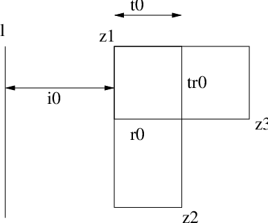
Since has Maslov index lower than and has a starting rectangle with , so induction applies finishing the proof. Thus in both the chains and , at some point we have to use a rectangle with and . But since and are increasing, and is the smallest value of that we can start with, we have to start with . Thus this fixes .
Now let us assume . We need an induction statement to show that is fixed. For each coordinate of , consider the horizontal line lying on some curve, which starts at and ends at and goes right throughout. We call to be admissible if every point just below the line belongs to . Since the starting rectangles in the chains and have , so there is at least one admissible coordinate. Among all the admissible coordinates, let be the one with having the smallest length. Let be the smallest length, measured by number of intersections with curves. Our induction claim is that at some point in any increasing chain we have to use a rectangle with and . The induction is done on the length of . Clearly when the length is , the claim is true. Let us assume we start with a rectangle with and . Since has index one, so it cannot contain any coordinate in its interior, and it also cannot contain any horizontal annulus. Thus it is easy to see that has to be disjoint from , and thus has Maslov index one lower than and still intersects and has an admissible coordinate with . Thus induction applies, and proves our claim.
Now it is easy to see that the starting rectangles in the chains and must have and . Since both are increasing chains, so we must start with a rectangle with . Now we want to show that is also fixed. This is also by an induction very similar to the ones above. Consider all with , such that the covering relation has . Let be the thinnest rectangle among all such covering relation, and let be the thickness of . The induction claim is that at some point in any increasing chain, we have to use a rectangle with and , and the induction is done on the length of . Again it is trivial when the length is . Assume we start with a rectangle with and . Since both and have index one, they must look like Figure 3.10.
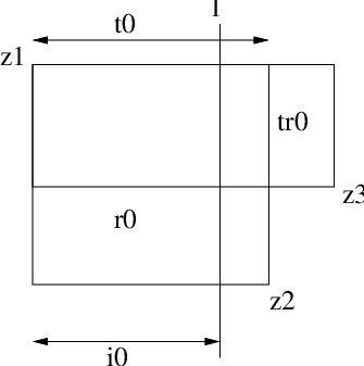
Note that has index one lower than and it still intersects , and it still has an admissible coordinate with . Thus induction applies. Since and are both increasing, this implies that they both must start with a rectangle with . Thus we see that the thickness is fixed.
As explained earlier, this finishes the proof. ∎
Using the theorems from section 3.1, this implies the following.
Theorem 3.3.4.
Each subinterval of an interval in the grid poset is shellable. For intervals of the form , the order complex is a sphere, and for intervals of the form , or , the order complex is a ball.
Thus using the results from Section 3.2, we see that , and (in each Alexander grading ) are GSS posets.
Now we concentrate the commutation posets and . Let be a commutation diagram. We are trying to prove that closed intervals in these posets are shellable. Once more it is enough to restrict our attention to closed intervals in .
Theorem 3.3.5.
Closed intervals in the commutation poset are shellable.
Proof.
We do not know if the closed intervals are always EL-shellable. We shall only prove that the closed intervals are shellable. For , let be a positive domain with . If and , we will prove that the closed interval is shellable. Note . So we prove this by taking cases.
Case 1: is the unique positive domain joining to and .
We can choose any vertical line disjoint from all circles (indeed we can choose a vertical line through ) and define as in the proof of the previous theorem. Essentially the same proof shows that this provides an EL-shelling. It is important to note that we can also apply the rotation (such that the horizontal commutation becomes a vertical commutation), and then take a vertical line (this time disjoint from all the circles), and then define which still induces an EL-shelling. The line has to be disjoint from and (which are now vertical circles), and we stipulate (for defining and ) that both of them are equidistant from .
Case 2: .
In this case, using Lemma 3.2.14, is the unique positive domain joining to . Choose a vertical line passing through , the chosen intersection point between and . To each covering relation, associate a -tuple , where , and are defined similarly and if the covering relation corresponds to a pentagon, and is otherwise. Thus given , and a -tuple , there is at most one with corresponding to that -tuple. The tuples are ordered lexicographically, and thus all maximal chains in have their edges labeled by a totally ordered set, and hence themselves get an induced total ordering. We claim this ordering gives the required shelling.
We follow the general outline of the proof of Theorem 3.1.4. Let and be two maximal chains, with . Let and agree from to and then start to disagree, and then agree once more at (and then maybe disagree again). Thus we can restrict our attention on the interval , which has a smaller length. Hence by induction, we will be done. Thus we can assume and , i.e. and never agree. The domain corresponding to might now have . But note is still the unique positive domain joining to , and hence if , then we have reduced this case to the previous case. Hence assume still has .
If has a subchain , where the -tuples corresponding to the two covering relations decrease, and the domain corresponding to does not look like any of the two domains in Figure 3.11, then we can change by replacing with with . Call such an operation a switching operation. A case by case analysis shows that the new maximal chain obtained after a switching operation is smaller than the original. Call the operation of changing one element of a maximal chain to get a smaller maximal chain, a generalized switching operation. Thus a switching operation is a generalized switching operation.

Since we are trying to prove shellability, hence we can assume that does not admit any generalized switching operation. In that case there is an element in , such that is an increasing chain in and is an increasing chain which starts with an empty pentagon but there is no such that the domain corresponding to looks any of the two domains like Figure 3.11. We call such a maximal chain to be quasi-increasing. Thus in a quasi-increasing chain, there exists and such that and the index domain corresponding to is one of domains shown in Figure 3.11. In all the cases, the -coordinates are marked.
Now we want to show that is the smallest chain. This will rule out the possibility of having a chain with , and thus finishing the proof. Thus, if possible, let . We can do the generalized switching operations as described above, on , such that also becomes quasi-increasing. Now if we show , we will have the required contradiction.
Thus we only need to show that there is a unique quasi-increasing chain. The proof is essentially the same as the proof of uniqueness of increasing chain in the previous theorem. Thus in this case, we are done.
Case 3: There are exactly two positive domains and joining to .
By assumption, note that both and have . Also both and must have . For simplicity, we apply the rotation . After rotation, all the circles (incl. and ) become vertical circles. Let be the domain which has non-zero coefficient in the region immediately to the left of . We choose the vertical circle to be line immediately to the left of and . We define as in the proof of the previous theorem. Note that we assume both and be to distance to the right of . Note that given and a triple there is at most one with corresponding to that triple. Thus each maximal chain gets a unique labeling. We use this labeling to totally order all maximal chains that come from , and also all maximal chains that come from . We then declare all maximal chains that come from to be smaller than all maximal chains that come from . We claim that this ordering is a shelling.
Again following the general outline of the proof of Theorem 3.1.4, let and be two maximal chains with . By restricting to smaller chains if necessary, we can assume that the two maximal chains are disjoint. After restricting to smaller chains, we can still assume that and are two distinct domains joining to , or else we have reduced this to an earlier case.
Now we can assume that is a non-decreasing chain, since otherwise we can do a switching operation to make it smaller. But each domain has a unique non-decreasing chain, which in addition is the smallest chain among all maximal chains coming from that domain. Since is a maximal chain which is smaller than , hence must be the unique non-decreasing chain coming from .
By assumption, the line lies entirely inside , and hence the first two covering relations in starting at must have as . Thus we can do a switch, where this index domain can be replaced another index domain, which is this domain minus , where is the special domain from Figure 3.7. After the switch, the new maximal chain comes from , and hence is smaller than . This completes the proof of shellability. ∎
Since the commutation poset was already a graded and signed poset, this completes the proof that it is a GSS poset. We now prove that the stabilization poset is also shellable.
Theorem 3.3.6.
The stabilization poset is shellable.
Proof.
In both and , even if we are allowed to pass through , the proof of shellability (indeed EL-shellability) follows directly from the proof of EL-shellability of intervals in the grid poset. There are only two cases which are slightly different.
The first case that is slightly different is when and . Here in any maximal chain, there will be exactly one covering relation corresponding to the trivial domain. Let us assign the -label to each of those covering relations as . It is easy to see that this labeling still induces an EL-shelling of the interval . In fact this interval is the Cartesian product of the posets and , where is a chain of length , and since each of the posets is shellable, their Cartesian product is shellable.
The other case that presents some difficulties is when and , and there are exactly two domains and joining to .
In this case, we proceed like the last case in the previous theorem. If , then we declare maximal chains coming from to be smaller than those coming from . For maximal chains coming from , we choose to be the vertical line passing through . We define in the standard way, and this induces a total ordering among all maximal chains coming from . For maximal chains coming from , we apply the rotation , and then choose to be the vertical line through , and then define to induce a total ordering among all maximal chains coming from .
We choose two maximal chains and with . We can assume that they are disjoint. If both of them come from either or , the proof is very similar to the proof of shellability of intervals of grid posets. Thus we can assume comes from and comes from . We can also assume that is the unique non-decreasing chain coming from . Thus the first two covering relations in must have as as their labeling, and hence we can modify that index domain by subtracting the vertical annulus through and adding the horizontal annulus through . After this switch, we get a maximal chain coming from , thus completing the proof of shellability. ∎
3.4. Applications
Given a grid diagram for a knot, the above theorems allow us to define some CW complexes. The constructions work for any GSS poset, but we only do it for the grid poset . (Here could be , or for any Alexander grading ). We start with the easiest construction.
3.4.1. Order Complex
We can give a CW complex structure on the order complex where the -cells are closed intervals of length . The boundary map maps to all the closed subintervals of length . The boundary map is well defined because the union of such subintervals forms a sphere of the right dimension.
Theorem 3.4.1.
The above defined CW complex is well defined and is homeomorphic to the order complex.
Proof.
Recall that the order complex of an interval of length is a ball of dimension . The order complex of the whole poset is just the union of all such balls, thus we only need to understand the boundary map. The boundary of the order complex of consists of all submaximal chains that are covered by exactly one chain, or in other words, maximal chains in and . But the order complex of each of and is a ball of dimension with common boundary the order complex of which is a sphere of dimension . Thus the order complexes of and glue to form a sphere of dimension , and is the boundary of the order complex . Thus the boundary map in the order complex is the same as the boundary map in our CW complex. This shows that the CW complex is well defined and is same as the order complex. ∎
3.4.2. Fake moduli space
Given a positive domain with , we construct a CW complex which has many properties of what the actual moduli space should have, although it is not clear whether the real moduli space will always be homeomorphic to this space. The -cells will correspond to the the maximal chains in , the -cells will correspond to the submaximal chains in containing both the endpoints, and in general an -cell will correspond to a chain in containing points including both the endpoints, and the unique -cell corresponds to the element chain . The boundary map is injective and is given by co-inclusion.
Theorem 3.4.2.
The above defined CW complex is well defined. It is homeomorphic to a ball, and its boundary is homeomorphic to the order complex of .
Proof.
Let us prove this by induction on , so assume the theorem holds for . By boundary of our CW complex, we mean everything except the top dimensional -cell. So by induction, the boundary of our CW complex is a -dimensional manifold . All we need to show is that is PL-homeomorphic to the order complex of . Once we have proved that, both being spheres of dimension , the attaching map of the -cell is forced, thus completing the induction.
Consider the order complex of . Its -simplices correspond to chains of length in . On the other hand is a CW complex whose -cells correspond to chains of length in . The boundary map of is same as the coboundary map of , which is given by inclusion. Since the order complex of is a manifold (in fact a sphere) of dimension , hence is just the dual triangulation of the order complex of . This completes the proof. ∎
3.4.3. Grid spectral sequence
We try to construct CW complexes whose boundary maps correspond to the grid homology boundary. This will ensure that the homology of the CW complex is the grid homology. We start with a very simple example. Consider the order complex of . It has a CW complex structure where the -cells are elements with and , and the boundary maps correspond to covering relations.
Theorem 3.4.3.
The above CW complex is well defined and is homeomorphic to the order complex of .
Proof.
For any with and , the order complex of is a ball of dimension , or in other words an -cell. The union of such cells make the order complex, thus we only need to show that the boundary maps are the same for the order complex and the CW complex. The boundary in the order complex corresponds precisely to the maximal chains in , or in other words maximal chains of where is covered by . Since being covered by in the grid poset is equivalent to saying that appears in in the grid homology boundary map, we conclude that the boundary maps for the order complex are same as the ones for the CW complex. ∎
In the later sections, we will constantly be dealing with pointed CW complexes, so now is as good a time as any to introduce them. spaces. In a pointed CW complex , the -skeleton is a point, which is the basepoint, but itself is not considered as a cell. If there are -cells, then the -skeleton is a discrete union of points. There are no attaching maps for the -cells. The construction of the rest of the CW complex is standard. We define a CW complex to be finite if it has finite number of cells. A finite CW complex is clearly finite dimensional.
We define a pointed CW complex to be nice if the following properties hold.
- •
There is a unique -cell (such that the -skeleton is a discrete union of points)
- •
The attaching maps for all the other cells are injective.
- •
We define a partial order on the cells of the CW complex and the basepoint, by declaring if . This poset is a GSS poset, with the grading being the dimension of the cell and the sign being the homological sign of the boundary map.
We can extend the above theorem and construct a pointed CW complex whose -cells correspond to elements with and whose CW complex boundary maps correspond to covering relations in .
Theorem 3.4.4.
For every , there is a well-defined pointed CW complex , such that the cells correspond to the elements of , the boundary maps correspond to the boundary maps of the chain complex induced from and agrees with any given sign convention on it, the cell corresponding to has dimension , and the boundary map every other cell is injective (which implies that is nice). We furthermore have .
Proof.
We extend the shellable poset by attaching elements , such that is covered by precisely the elements that cover and with the same sign for each covering relation, and each of and is covered and with positive and negative signs respectively. Using Lemmas 3.1.2 and 3.1.3, we see that this new poset is also shellable. Let be the poset defined as .
Now consider the order complex of . It has a CW complex structure whose cells correspond to the elements of , and the boundary maps represent the covering relations. But is a thin shellable poset, and hence the order complex of is a sphere of dimension . Thus we can treat the order complex of as the cell corresponding to in our pointed CW complex. The order complex of then has a pointed CW complex structure, whose cells correspond to elements of and whose boundary maps correspond to the chain complex boundary maps.
Recall that a sign convention assigns or to each covering relation in the poset . Two sign conventions are said to be equivalent if one can be obtained from another by reversing the orientation of all the the covering relations , where exactly one of and belong some fixed subset of generators. A property that sign conventions must have is that the grid homology boundary map must actually be a boundary map. This means if is an interval of length three, then the product of the signs of the four covering relations is .
Note that the boundary maps in the CW complex also has this property and this equivalence. The equivalence is obtained by reversing the orientation of the cells corresponding to the fixed subset of generators. To see that it also has the above mentioned property, let be an interval of length three. The generator will correspond to an -cell, whose boundary will contain two -cells corresponding to and . These two cells have a common -cell on their boundaries, coming from . Thus it is easy to see that the product of the signs of the four boundary maps has to be negative.
Now we will show that this equivalence and this property is enough to determine the sign in . Fix a maximal tree in the graph . Using the equivalence, we can ensure that all the edges in this maximal tree have positive sign. Now, we need to show that the property will fix the sign of every other edge. Whenever we add an edge, we get a cycle in the graph , consisting of that edge and a few edges from the maximal tree. If we can show that any cycle is generated by -cycles coming from intervals of length three, then we are done.
Consider two maximal chains in . They combine to form a cycle. Call such cycles to be simple cycles. It is easy to see that any cycle in is a sum of simple cycles. So we only need to show that any simple cycle is a sum of -cycles coming from length three intervals. Let and be two maximal chains in . Since is shellable, it follows from definition that there is some total ordering on the maximal chains, such that we can replace the bigger maximal chain by a smaller one after modification by a -cycle coming from a length three interval. This completes the proof that there is a unique sign assignment on and hence we can choose the orientations of the cells properly to ensure that the CW complex boundary maps respect the sign conventions.
Also note that during the construction of the CW complex, when we were trying to attach an -dimensional cell, its boundary had to map injectively to an -sphere respecting some sign. Thus throughout there was only one option, and hence there is only one such CW complex that can be constructed with the above properties. This shows that the CW complex is well-defined. Since with the obvious CW complex structure, is another CW complex with the same properties, we have . ∎
Indeed, the above proof shows that if with , then the -ball has a pointed CW complex structure, whose cells are the generators in and the boundary maps are the grid homology boundary maps. This has the following corollaries.
Lemma 3.4.5.
For any interval with , the the homology of the chain complex induced from the poset, is trivial.
Proof.
The homology of the chain complex induced from is the reduced homology of the pointed CW complex whose cells correspond to the generators of and whose boundary maps correspond to the chain complex boundary map. However since that CW complex is the ball, hence the reduced homology is trivial. ∎
Lemma 3.4.6.
There are even number of generators with .
Proof.
We can assume . Consider the chain complex induced from the poset . Since it has trivial homology, there must be even number of generators in , and hence in . ∎
We digress for a bit to explore some consequences of the previous lemma. For the rest of this subsection, we work with coefficients in . The grid homology boundary map can be written succinctly as
Let us generalize this map to define
The above lemma implies that for any , . Choosing tells us that is a chain complex, with homology say . Choosing tells us that is well defined on , and choosing tells us that is a chain complex with homology say . In general is a chain complex with homology . Thus we see that this in fact defines a spectral sequence starting with the grid homology. The following suggests that it is not a very exciting one.
Lemma 3.4.7.
The second map is zero on .
Proof.
Let be a homogeneous element in . Thus is a linear combination of generators from . Recall that we are working with coefficients in , thus simply corresponds to a collection of generators, all with the same grading. We are also assuming . Let be the collection of generators which are covered by some element from . Similarly let be the set of elements which are covered by some element of . Let . Note that is a subset of . We will show that there exists a subset of , such that . That would imply that is zero in .
Since , each element of is covered by an even number of elements from . Let be the set of elements in that are covered by mod generators from . We claim . Choose an element . We now consider the set . It is easy to see that there are even number of elements in this set, and half the cardinality of this set has the same parity as the number of elements in that cover , and also the same parity as the number of elements in that are bigger than in the grid poset. Thus appears in if and only if appears in . This concludes the proof. ∎
Note that the above proof can easily be generalized to show that if is a homogeneous element in with and , then there exists a homogeneous element in such that . It is not clear whether this is enough to show that all the higher ’s vanish.
3.5. CW complexes
In the previous section, we defined a nice CW complex to be a pointed CW complex with a unique -cell, such that the attaching maps for all the other cells are injective, and the poset whose elements are the cells and the basepoint is a GSS poset. Hence the order complex of any closed interval of the poset is a ball, and the order complex of any interval of the form is also a ball.
In fact, using Theorem 3.4.4, given a suitable GSS poset, there is one and only one nice pointed CW complex satisfying these properties. Furthermore, we can fix the orientation of the -cell arbitrarily, but once that orientation is fixed the orientation of every other cell and the basepoint is fixed by the sign convention of the GSS poset.

Let be a nice finite CW complex. Let the dimension cells of be . We define its dual in the following way. We first fix a map from the discrete union of all cells to , such that each cell maps to a single point in , and different cells map to different points in . Let the image of the cell be ; let be the straight line path from the origin to at constant speed, and let be the graph of the function .
Given such a map , we will construct a PL-embedding of in , with , where is the dimension of . We will embed the -skeleton in , and then view as the subspace in and extend this embedding to the -skeleton. Thus we will be able to embed in which we view as the subspace in .
Theorem 3.5.1.
Given a map , there is a PL-embedding of the type as described in the previous paragraph.
Proof.
For clarity, we explicitly write down the embedding of for a few small values of . We embed the -skeleton in by mapping the basepoint to the origin and the -cell to .

The -cells are . We view as , and embed as an union of for , and . Note that since ’s are distinct, this is indeed an embedding.
There is a different way of viewing the above process. For each -cell , its boundary is a -sphere in , and bounds a disk in (which in our case always happens to be the unit interval ). We then embed the -cell as a union of an annulus embedded in as , and a disk embedded in as .
Now to embed in , we proceed inductively. We assume is already embedded in , and we view . For each -cell , its boundary is a -sphere embedded in . If that sphere bounds a disk in , then we can embed the -cell as an union of an annulus embedded in as , and a disk embedded in as . Note that since ’s are distinct points in , this is still an embedding.
Thus to show that there is a well-defined embedding depending only on the choice of the map , we need to produce a disk bounding , which does not depend on anything other than the choice of the map . Without loss of generality let . Let be the boundary of a -cell . Note that the order complex of is a disk of the same dimension as . So we will produce an embedding of this order complex with the proper boundary.
To present a clearer picture, let us explicitly describe how we define the embeddings of the vertices and edges of this order complex. We embed and as and respectively. For , we embed as . The edge joining to is , the edge joining to is , the edge joining (resp. ) to is followed by (resp. followed by ).
Now let us describe in general how a simplex of this order complex coming from a chain is embedded in with . We embed this as the disk . For the rest of this paragraph, let us call this subspace as , where is a subspace of . The simplex of the order complex coming from the chain is a suitable part of the boundary of the above order complex, and again for the rest of this paragraph, let us denote that subspace to be , where is a subspace of . Then the simplex of the order complex coming from a chain is embedded as the union of followed by and the simplex of the order complex coming from a chain is embedded as .
Thus we have embedded the order complex of in , and this is the required disk bounding . Using such disks ’s, we can then embed in , thus completing the proof. ∎
There are a few observations that we should make now. The only choice we made in defining the embedding is the choice of the map . But we can connect any two such maps and by an isotopy of , and this induces an isotopy in connecting the embeddings and .
Furthermore, this embedding is also an embedding of the order complex of the whole poset coming from the CW complex. The basepoint is embedded as the origin, the -cell is embedded as , and the vertex corresponding to the cell is embedded as . A simplex of this order complex coming from a chain is embedded in , as the disk . Once more for the rest of this paragraph, let us call this subspace as , where is a subspace of . The simplex of the order complex coming from the chain is a suitable part of the boundary of the above order complex, and again for the rest of this paragraph, let us denote that subspace to be , where is a subspace of . Then the simplex of the order complex coming from a chain , where is the basepoint, is embedded as the union of the closure of , followed by followed by . Note that this embedding of the order complex is slightly different from the one that we used in the previous proof.
Thus the closure of a regular neighborhood of in will give an -dimensional manifold (with boundary) with same homotopy type as that of . We construct in the following way. Let be the set of all points with distance less than or equal to from . We assume ’s are decreasing in and we choose positive to be small enough such that the interior of is a regular neighborhood of . For each (resp. ), after we have already chosen we choose positive to be sufficiently small such that has exactly one component (resp. exactly two components) for each -cell . We define . Note that is not a smooth manifold.
Let be the image of the basepoint in the embedding, and let be the small neighborhood of , lying in the interior of . Let us view as a cobordism from to . Note that this cobordism is obtained by starting with , adding disks corresponding to the embeddings of the order complexes of , and then taking a regular neighborhood. Now let us assume that there is a Morse function and a corresponding gradient-like flow for this cobordism, such that the flow is transverse to and , the only index critical points are the images of the vertices in the order complex corresponding to and the left-handed disks are the embeddings of the order complexes corresponding to . Then the original pointed CW complex can be recovered from this gradient-like flow in the following way. Quotient out to the basepoint, and the cells for the CW complex are the left-handed disks with the attaching map being given by the flow. We construct the dual of in a very similar way. We look at the right-handed disks, and regard the cobordism as obtained from by adding those disks and then taking a regular neighborhood. Thus to construct the pointed CW complex dual to , we should quotient out to the basepoint, and have cells correspond to right-handed disks with attaching maps given by the flow. However to define the dual in this way, we first need to find a Morse function and a corresponding gradient-like flow satisfying the above conditions. The dual then might depend on the choice of the Morse function and the gradient-like flow and also on the map . We will bypass the construction of the Morse function and the gradient-like flow, and define the right-handed disks directly, depending only on the choice of the map .
We will define the right-handed disk corresponding to the critical point coming from the vertex of the order complex in several stages. Recall that the regular neighborhood is constructed as a union . Let . We will define starting at , then gradually extending the definition to , and finally define .
Furthermore, note that for . So for , we only need to define . We define as the connected component of not containing . For , define as the intersection of with the hyperplane and extend to as the set of all points in whose distance from (embedded as ) is at most . It is easy to see that lies in the union of and and each right-handed disk is still a ball of the correct dimension. The way we extended the definition of to that of can also be described as follows. Since is one of the components of , is a disjoint union of -dimensional balls, one for each . We then take the ball corresponding to and extend it like a horn in the direction of until we reach the vertex corresponding to . Since different balls on corresponding to different ’s are disjoint, after extending the horns, is still a ball of dimension . Suitable parts of are defined as .
Now to define , by induction, let us assume, we have defined for all . We define as the intersection of with the plane . For , by induction is already defined. is a disjoint union of -dimensional balls, one for each with . We extend the ball corresponding to in the direction given by embedding of the order complex of until we reach the boundary of the order complex. We define as after these extensions. Since was a -dimensional ball, and we extended along disks starting at different portions of , is still a ball of the correct dimension. Note that is still the set of all points in whose distance from is at most , and thus it is particularly easy to see that is an -dimensional ball, since is an -dimensional manifold. Finally, we define . Note that lies in the boundary of if and only if and in that case, it is actually embedded.

We then quotient out to the basepoint, and define the dual CW complex using the right-handed disks as described above. Note that the union of all the right-handed disks is simply , and thus if , we can also construct the dual by starting with and then quotienting out to the basepoint. This construction might a priori depend on the map , but we can connect any two such maps and by an isotopy of . During the isotopy, for each (resp. ) we can make the ’s used in the definition of ’s sufficiently small such that the condition about having exactly one component (resp. exactly two components) for each -cell holds. Then this induces an isotopy joining the two ’s, and hence induces a homeomorphism between the two duals. Thus the dual of a nice pointed CW complex does not depend on the map and depends only on the ambient dimension . Let us denote this dual by .
Before we prove any other properties of the dual, we need to understand the dependence of on . The following result makes this precise.
Theorem 3.5.2.
For a nice pointed CW complex , we have , where denotes the smash product.
Proof.
After fixing a map , we can construct an embedding of in in a well-defined way, and we extend this embedding to an embedding into by embedding into as . After fixing an embedding to , we define as a pair with lying in , and we define as a quotient of obtained by quotienting out to the basepoint.
However is homeomorphic to and is homeomorphic to . Since is the circle , hence . ∎
Now we are in a position to state and prove the following important properties of duals. Let be a nice pointed CW complex, and let be a subcomplex. is also clearly nice and pointed. We can thus define the duals and for sufficiently large (in fact simply has to be larger than where is the dimension of ). Then the following holds,
Theorem 3.5.3.
For a subcomplex of a nice CW complex , the dual can be obtained from by quotienting out the cells corresponding to the cells in that are not in .
Proof.
Note that it is enough to prove the case when there is exactly one cell that is in but not in . Thus to embed in , we embed in and then delete the cell (which was embedded as an embedding of the order complex of ). Another way to see this is the following. Take the embedding of , view it as an embedding of the order complex, and delete the vertex corresponding to . Then the new space deform retracts to the embedding of . Let and be regular neighborhoods of and respectively, as defined earlier in this section. Let be a small neighborhood of the right-handed disk of in the embedding of . Then deform retracts to .
The right-handed disks required for defining the dual come from the manifold . The right-handed disks required for defining the dual come from the manifold , and when these right-handed disks are restricted to , they define the quotient complex of obtained by quotienting out , the cell corresponding to . A properly chosen deformation retract of to gives the required homeomorphism between this quotient complex and . ∎
A very similar property holds for quotient complexes. However if is a nice pointed CW complex, quotient complexes of in general will not be nice. Let be an -cell of , and consider the quotient complex of obtained by keeping only the cells with and quotienting out everything else. Let us assume that there is a nice pointed CW complex , such that with the natural CW complex structure is the same CW complex as (in fact using Theorem 3.4.4, we can always assume this). If is the dimension of , then for , we can define the duals and . Then the following is true.
Theorem 3.5.4.
The dual is homeomorphic to the subcomplex of obtained by considering only the cells corresponding to the ones present in .
Proof.
First observe that the order complex of the poset coming from restricted to the cells of , can also be obtained from the order complex of by removing the element corresponding to the basepoint. Now choose an embedding of (which is also an embedding of the order complex of the poset coming from ) to . Let us restrict to the order complex of , where is the basepoint in , and delete all the simplices which use the edge coming from . This is same as the order complex coming from . Thus an embedding of in gives an embedding of this order complex in . We will now modify this embedding such that it agrees with a standard embedding of in . Observing how the right-handed disks change under this modification will complete the proof.
At time for , is embedded as , the basepoint is embedded as and a vertex for is embedded as . The simplex coming from a chain that does not involve is a shifted version of the original, with the second, third and fourth coordinate being changed from to . The simplex coming from a chain that involves is a truncated version of the original, where we delete the part that intersects with . Note that at , this is an embedding of the order complex of as induced from an embedding of . At , this is the standard embedding of the order complex of in . To complete the proof, we should observe how the right-handed disks change during this isotopy. At time , we can define the right-handed disk of as a truncated version of the original right-handed disk by deleting the part that intersects with and the right-handed disk of for as a shifted version of the original right-handed disk with the second, third and fourth coordinate shifted from to . This gives an explicit isotopy connecting the subcomplex of coming from the cells corresponding to those in , to ∎
Thus given a GSS poset with one minimum, by Theorem 3.4.4, we can construct a nice CW complex corresponding to the poset, and then construct its dual. We can assign an orientation to the top dimensional cell (the one corresponding to the unique minimum in the poset) arbitrarily, but once that is fixed the orientation of the rest of the cells is determined by the sign convention on the GSS poset. This extra information coming from the orientation of the top-dimensional cell allows us to strengthen Theorem 3.5.4. In that theorem, we showed that there is an isomorphism between and a subcomplex of , but there might be more than one such isomorphism. However after we orient the top-dimensional cells in both and (and hence using the sign convention on the poset of , orient every cell in these two CW complexes), we choose the isomorphism that matches the orientations. Thus for oriented CW complexes, there is a well-defined isomorphism between and a subcomplex of . This will be of use to us in Section 3.6.
Before concluding this section, we should note that our explicit construction of a dual actually agrees with the Alexander dual, which is obtained by embedding the space in the sphere , and then taking the homotopy type of the complement. Thus the Alexander dual is homotopic to . The way to see this is as follows. Let us embed as described above into and let be viewed as the one point compactification of that with that extra point being denoted by . Let be the basepoint in the dual and let be the Alexander dual. If denotes the homotopy equivalence of pairs of spaces, we have
However we have an exact sequence of spaces
This induces the Puppe map from to , and since , the map induces isomorphism in and hence induces a homotopy equivalence.
3.6. Grid homotopy
Let be a GSS poset. For most of the time, will be a grid poset, a commutation poset or a stabilization poset.
If we take the poset , and reverse the partial order, observe that each closed interval in the new poset is still shellable. This follows from the definition of shellability. Thus the applications of Section 3.4 can all be constructed. In particular, we can construct a pointed CW complex corresponding to the interval in the old poset, whose cells are elements of and the attaching maps correspond to the coboundary maps in the chain complex induced from the poset.
Theorem 3.6.1.
There is a well-defined nice CW complex , such that the cells correspond to the elements of , the boundary maps correspond to the coboundary map of the chain complex induced from and agrees with any given sign convention on it, the cell corresponding to has dimension , and the boundary map every other cell is injective.
Proof.
We reverse the partial order of the poset and construct the pointed CW complex as described in Theorem 3.4.4. This is the required pointed CW complex . ∎
We now state and prove the main result of this section.
Theorem 3.6.2.
Given a GSS poset , for sufficiently large , there is a well-defined CW complex whose -cells correspond to the elements of of grading and whose boundary maps correspond to the covering relations in even up to sign.
Proof.
If and are the maximum and the minimum gradings in the poset, then we choose . For each , we construct as in the Theorem 3.6.1. Each of these CW complexes is a nice pointed CW complex, and hence we can construct their duals where is the grading of . In each of these CW complexes, we orient the top-dimensional cell arbitrarily, and that fixes an orientation of every cell. For , is a subcomplex of . A repeated application of Theorem 3.5.4 allows us to construct a well-defined injection of to which matches the orientations. Thus we have a space for each and a map for each pair with . We take the discrete union of all these spaces and glue them together using these maps and call it . It is easy to see that is well-defined and satisfies the conditions of the theorem. ∎
However note that the same poset can carry two different non-equivalent sign conventions. Figure 3.15 demonstrates that such posets can indeed give rise to different spaces. In the diagram we have significantly reduced the dimensions of the spaces.

Now we want to state and prove certain properties of this space .
Theorem 3.6.3.
If is a GSS poset, is a subposet and is a quotient poset, then for sufficiently large, the following are true.
.
is a subcomplex of containing only the cells corresponding to the elements in .
is a quotient complex of containing only the cells corresponding to the elements in .
Proof.
Thus by taking to be , or (for any Alexander grading ), and for sufficiently large, we can construct CW complexes . In fact for sufficiently large, , where is the wedge sum.
Since we can associate finite spectra to each GSS poset , whose -th space is . The previous note implies that . We can also define a spectrum corresponding to by defining it to be .
Now we want to show that some of these objects that we associate to grid diagrams of knots are actually knot invariants. First note that any two grid diagrams for the same knot are related by a sequence of commutations and stabilizations. We will consider each of the cases in great detail.
3.6.1. Commutation
Theorem 3.6.4.
If two grid diagrams and differ by a commutation, then for any Alexander grading , and with sufficiently large (resp. ) and (resp. ) are homotopic.
Proof.
For the rest of the proof, let (resp. ) denote or (resp. or ) as the case may be. With similar conventions, let be the relevant commutation poset.
Since is a subcomplex of and is the corresponding quotient complex, we have a long exact sequence of spaces
This induces the Puppe map from to . As proved in [MOST07], this map induces an isomorphism in homology, and since we can choose large enough to ensure that both the sides are simply connected, the map is a homotopy equivalence. ∎
3.6.2. Stabilization
The situation for stabilization is slightly different. For the case of we can no longer hope for any sort of homotopy equivalence.
Theorem 3.6.5.
If and are the grid diagrams before and after stabilization, then for any Alexander grading and sufficiently large, (resp. ) is homotopic to (resp. ).
Proof.
In case (resp. case ) of the stabilization, both and have a subcomplex (resp. quotient complex) corresponding to either one or two copies of the complex for and the corresponding quotient complex (resp. subcomplex) corresponds to the complex for . Following the lines of the previous proof, we observe that these spaces then fit into an exact sequence. Thus the Puppe map gives a map between the two spaces corresponding to the two complexes. This map induces a chain map between the two complexes. Thus if both sides are stabilized sufficiently so as to ensure that they are simply connected, and if the Puppe map induces isomorphism in homology, then the Puppe map would be a homotopy equivalence. Thus we only need to show that the map induced in homology is an isomorphism.
Following the lines of the proof in [MOST07], we prove that it is a quasi-isomorphism. Note that since we then prove that this map is induced from a homotopy equivalence of spaces, the map actually becomes a chain homotopy equivalence.
We fix some Alexander grading , and only work with generators of that grading. On (and hence on and ), we introduce additional filtrations given by powers of . We then put special markings on every square of other than the ones on the vertical or the horizontal annulus through . On the associated graded object, obtained after the filtration by the powers of , we put an additional filtration by counting how many times a domain passes through the extra markings. We call this filtration , and on the associated graded objects of we put an additional filtration given by sum of powers of and . (Note that while working in the hat version, the filtrations coming from the powers of ’s are unimportant).
Restricted to the generators coming from , the objects in the associated graded object of are similar in the hat version and the minus version. For now, we concentrate on the associated graded object in after the filtration . We only work with case of the stabilization. Similar results hold true for case after the rotation , but some of the maps are in the opposite direction.
Recall that is the intersection between and . Let be the intersection point immediately to the right of . Let (resp. ) be all the points in whose one of the coordinates is (resp. ). We name the (resp. ) circle just below (resp. right of ) as (resp. ). Let be all the generators which do not have any coordinate among the points of intersection among . All the other types of generators are shown in Figure 3.16.

Note that (resp. ) consists of (resp ), (resp. ) and the special generator (resp. ). After the filtration domains have to lie in the union of the horizontal and the vertical annulus through and are not allowed to pass through . Hence the chain complex decomposes as a direct sum of the chain complexes , , , , , and , where (resp. ) consists of the generators from and (resp. and ). It is easy to see that the homology of is zero, and there is no differential in the next summands. The differentials in map one element (say ) of and one element (say ) of to one element of , and the differentials in map one element of to one element in (say ) and one element of (say ). Thus the homology of (resp. ) is freely generated by elements like (resp. or ).
This gives us the generators for the homology of the associated graded object of after the filtration . We want to show that the map coming from the covering relations between elements of and in is a quasi-isomorphism. For that it is enough to show that the map induces isomorphism on the homology of the associated graded object of . This is easy, since the map from to (resp. ) maps to and is a bijection from to and from to (resp. induces identity map on and maps to ). Note that this is independent of the sign convention chosen.
For the minus version we have to do a little bit more work. Let us use the shorthand to denote terms of the form . The domains are now allowed to pass through and , and due to the result of the previous part, we are only interested in domains connecting elements of the form or to elements of the form or .
For the special generator , there are domains connecting to and . Thus if we consider all the generators of the form with and all the generators of the form with , the chain complex looks like Figure 3.17 and it is easy to see that the homology is carried by , irrespective of the sign convention.

For a generator , the domains connect to and for some generators and . Since is same as in the homology of the associated graded object of , hence the diagram once more looks like Figure 3.17. Thus the homology is again carried by .
Similarly, for a generator (resp. ), there is only domain connecting (resp. ) to (resp. ) for some generator . A similar argument shows that the homology is once more carried by .
Thus the homology of the associated graded object is freely generated by elements of the form . The map which we are trying to show is a quasi-isomorphism induces a bijection between elements of that form and generators of . This completes the proof of the fact that the relevant maps are quasi-isomorphisms, and as argued earlier this completes the proof of the theorem. ∎
Thus to every knot and every Alexander grading , we can associate an invariant spectrum , and hence after taking an infinite wedge, the spectrum . We call these spectra and to stress the fact that they only depend on the knot , and not on the grid diagram representing . Thus any invariant of the spectrum is also a knot invariant. The homology of the spectrum is the well-known invariant . Stable homotopy groups can constitute an interesting collection of invariants. Another invariant to consider is the Steenrod operations. For simplicity, let us just consider the operation acting on the cohomology with coefficients which increases the grading. Since cohomology of is same as where is the reverse of the knot (the isomorphism being obtained by applying a rotation on a grid diagram for the knot ), the Steenrod squares act on by reducing the grading.
A very natural question is whether computes anything new. It will interesting to find two knots and , such that and have the same homology, but are not homotopic to one another.
For the hat version, unfortunately we do not have a knot invariant. Given an index grid diagram for a knot we can construct finite spectra and their wedge .
It is not clear whether the homotopy type of these spectra depend only on and . However there is some partial answer to this question. Let be the highest Alexander grading such that the homology of is non-trivial. It is easy to see that depends only only the knot . Then we claim that the homotopy type of the spectrum also depends only on the knot , and henceforth we will denote it by . The way to see this is as follows. For sufficiently large and , the spaces are acyclic as they are simply connected and have trivial homology. Commutation does not change the homotopy type of , and when we stabilize to go from a grid diagram to a grid diagram , for sufficiently large , we have since the second space is acyclic.
In fact this proof shows a possible way to answer the above question positively. We are trying to show that the homotopy type of depends only on , the Alexander grading and the grid number . First note that it is enough to prove the following fact. If the stabilizations of and have spectra that are homotopy equivalent, then the spectra for and are homotopy equivalent. We have already proved this for . So by induction assume it is true for all Alexander grading bigger than . Thus for sufficiently large, we have . But by induction, we already know . Thus our proof would be complete if for finite CW complexes , and , being homotopic to would imply that is stably homotopic to .
However, irrespective of that, we can still construct certain stable homotopy invariants from the spectra which depend only on and . One such example is the stable homotopy groups.
Theorem 3.6.6.
The stable homotopy groups of depend only on , and .
Proof.
We just mimic our attempted proof for showing the homotopy type of depends only on , and . Call two grid diagrams and to be -equivalent if after stabilizing both of them times, the two diagrams can be related by commutations. We are trying to prove that for two -equivalent diagrams and . This is true if either or the Alexander grading is sufficiently large. We prove this by an induction on the pairs ordered lexicographically.
If two diagrams and are -equivalent, then their stabilizations are -equivalent, and hence from the induction on , we get . However for spectra coming from finite CW complexes, the stable homotopy groups are finitely generated and abelian, and for wedges, they are products, and hence (using the classification of finitely generated abelian groups) we get . ∎
3.7. Examples
In this section we give examples of some other GSS posets , and construct the spaces corresponding to them. We will conclude the section by computing the homotopy type of for the grid diagram of the trefoil as shown in Figure 3.18.

As a warm-up exercise, let us first consider the crown poset . In this poset there is a unique minimum (resp. unique maximum ), which is covered by the elements (resp. which covers ). Furthermore, each is covered by and with the counting done modulo . This can be made into a graded poset by assigning gradings of and to , , and respectively.
There is also a sign assignment which assigns to each edge that involves either or , and to each edge of the form and assigns to every other edge. Since the poset has a unique minimum, this is the unique sign assignment (this actually follows from the fact that is shellable).
It is easy to check that this poset is also shellable. Let us draw a graph whose vertices are maximal chains, and there is an edge joining two vertices if and only if the two maximal chains agree at exactly elements. It is clear that the graph is a -cycle. Let us now delete one of the edges of this graph, and put a direction on the remaining edges, such that there is at most one edge flowing into a vertex and there is at most one edge flowing out of a vertex. The shellable total order that we put on the maximal chains is the following. We declare a maximal chain to be smaller than a maximal chain if we can go from to along directed edges in the modified graph. It is easy to check that this ordering suffices.
Thus is a GSS poset and we can associate a pointed CW complex to it such that the reduced homology is the homology of the chain complex associated to . However it is immediate that the chain complex has trivial homology, and hence for sufficiently large , is a simply connected space with trivial homology and hence is homotopic to a point.
Now let us consider some other families of examples. Let be the poset of two elements and , with . Let be the -fold Cartesian product of with itself. For very natural reasons, let us call this the -cube poset.
The elements of look like -tuples where each is or . We put a grading on this poset by declaring the grading of to be the number of ’s in the -tuple. We can also put a sign assignment on this poset in the following way. Observe that if , then there is a unique for which and , and for every , . We assign a sign of to this covering relation, and it is easy to check that this is indeed a sign assignment. Since there is a unique minimum, this is the only sign assignment up to equivalence.
This poset is also EL-shellable. In an edge , if is the unique place where , we label the edge by the integer . It is easy to see that this map from the covering relations to integers totally ordered in the standard way, is indeed an EL-shelling. However once more since the homology of the chain complex associated to is trivial, the CW complex is contractible for sufficiently large .
The -cube poset is naturally isomorphic to the subset poset, whose elements are subsets of partially ordered by inclusion. An element of corresponds to a subset , such that if and only if .
Now consider the -cube poset restricted to the elements of positive grading. Let us reduce the grading of each element by , and then rename it as the simplex poset since the grading elements of this poset correspond to -simplices lying inside an -simplex , with partial order being given by inclusion. Thus is graded with -simplices having grading . It has a sign assignment obtained by restricting the sign assignment of the subset poset, and this is the unique sign assignment, since has a unique maximum. It is also shellable, since it is isomorphic to the interval of the subset poset. So is a GSS poset.
We can also construct the reduced simplex poset , where we label one of the vertices of the -simplex to be the basepoint , and define with the same partial order. This poset also has grading and sign assignments, and each closed interval in this poset is still shellable since closed intervals in the poset are shellable. Thus is also a GSS poset.
Theorem 3.7.1.
For large enough, there is a well-defined homeomorphism between and , where is the one-point compactification of with being the basepoint.
Proof.
Let be the maximum element in . Since the poset is shellable and thin, its order complex is . After reversing the partial order, if we recall the construction from Theorem 3.4.3, then we see that this partially ordered set comes from a CW complex structure, whose -cells correspond to elements of grading . However can also be thought of as the boundary of the -simplex with the inherited simplicial structure where -cells correspond to elements of grading . It is relatively easy to check that this is the dual triangulation of the CW complex structure.
Now recall how is defined. We embed the order complex of the reverse of into in some standard way. We take the image of the point corresponding to (denoted in Section 3.5 as ), and construct the first step of its right-handed disk which is simply an -dimensional ball . We extend to by marking some thickened -cells lying on , one for each element of grading in . Finally, we quotient out everything in that is not marked, to a point to obtain .
Thus we are embedding with the CW complex structure as described in the first paragraph into , taking a regular neighborhood of that in , and then quotienting out its complement in to a point to obtain . But the dual triangulation of that is the simplicial complex , and since is sufficiently large, this embedding of in can be extended in a standard way to a proper embedding of in . For for large enough, we then can view as , where is the -dimensional disk, with the closure of the regular neighborhood of in being . The space is obtained by quotienting to a point. This is illustrated in Figure 3.19 for and .

We end the proof by noting that
∎
Theorem 3.7.2.
For large enough, there is a well-defined homeomorphism between and , where is the basepoint in .
Proof.
We construct in a similar way. View as a quotient poset of and let be the maximum element of . We embed , the order complex of the reverse of (which itself is being thought of a subposet of ) into , the boundary of . We know that the dual triangulation of is the simplicial structure on , and for large enough we can view as , with being embedded as , and the closure of its regular neighborhood being .
However, since we are working with , we actually embed the reverse of , now thought of as a subposet of . This order complex is minus the -dimensional cell corresponding to the vertex in . Thinking in terms of the dual triangulation, it is , where is a small neighborhood of the basepoint . The complement of a regular neighborhood of this order complex in can be thought of as . We obtain by starting with and then quotienting out to a point.
We once more end the proof by noting
∎
For the next theorem, let denote either or depending on whether contains a special marked vertex or not. Similarly let denote either or , and correspondingly let denote either or .
Theorem 3.7.3.
Let be a codimension- face in . There can be three cases regarding the role of the basepoint , namely, , or . In either case for sufficiently large , the following diagram commutes
where the inclusion on the left is given by Theorem 3.6.3, and the inclusion on the right is induced from the inclusion of into .
Proof.
Let us just do the case when . Recall that is obtained from by quotienting out . However the inclusion of into induces both the inclusion on the left and the one on the right, and hence the diagram commutes. ∎
The above theorems have a very interesting corollary which shows that the CW complexes can be quite complicated.
Theorem 3.7.4.
Let be a simplicial complex with a special vertex marked as the basepoint . Then there exists a GSS poset , such that for sufficiently large , .
Proof.
Let us construct a poset whose elements in grading are the -simplices of partially ordered by inclusion, and then delete the element corresponding to . Let us also fix an orientation on every simplex of , and then assign signs based on whether the attaching map preserves orientation or reverses it. The closed intervals in this poset are isomorphic to the subset poset, and hence are shellable. Thus is a GSS poset. For large enough , let us consider the pointed CW complex .
The -cells of correspond to -cells in , and the boundary maps of correspond to the boundary maps in . Observe that with its natural pointed CW complex structure also has this property. Now recall how we construct . For each element , we construct a CW complex corresponding to the poset , and whenever , there is an embedding of the CW complex corresponding to into the CW complex corresponding to . Since such an inclusion can be viewed as a composition of inclusions coming from covering relations like , we can just restrict our attention to those maps.
If corresponds to an -simplex, then the poset is either or depending on whether or not is in . From the previous theorems, we know that the CW complex corresponding to is either or , and the inclusion maps coming from are induced from inclusions of simplices in . Thus and have the same CW complex structure, and hence are homeomorphic. ∎
Theorem 3.7.5.
There exist GSS posets and with the same homology, but with different homotopy types of their associated spectra.
Proof.
We want to find GSS posets and with same homology, such that is not homotopic to for all . We choose to be a poset consisting of only two elements, which are non-comparable and have gradings and . We choose to be poset coming from a simplicial complex structure on . Clearly both have homology supported in gradings and .
Furthermore, and . We want to show that these two spaces are not homotopic for any , or in other words, we want to show that is not stably homotopic to . This can be seen in several ways. If and (resp. and ) denote the generators in and of (resp. ) with coefficients in , then but , where is the second Steenrod square operation. Also and , where is the third stable homotopy group. ∎
Now as promised at the beginning of the section, we do the computation for the hat version of the trefoil presented in the grid as shown in Figure 3.18. We use the notation to denote the element which contains the points of intersection between the vertical lines marked and the horizontal lines marked . By components of , we mean path connected components of the graph that represents the partial order on . A simple computation shows that there are components in of which of them contain only one element. There are two components and with elements each, and homology , and there is one component with elements and homology .
The CW complex is a wedge of the CW complexes coming from the different components. The spaces coming from the components with only one element are simply spheres of the right dimension, so we can restrict our attention to and . Let us first consider the case of .
Each of and has a unique element of maximum Maslov grading (however neither of them have a unique maximum), which happens to be and respectively. However these two generators swap when we apply a rotation of and reverse the roles of ’s and ’s (which can be done in the hat version). This shows that is isomorphic to as posets and hence we can work with . The following are the elements of .
- •
Maslov grading :
- •
Maslov grading : , , , ,
- •
Maslov grading : , , , , , , , , , , , , , ,
- •
Maslov grading : , , , ,
The homology lies entirely in grading . There are six maxima in which are , , , , in grading and in grading . Let be the poset which turns out to be . Since is a subposet of , is obtained by adding five -cells to . However the homology of is in grading , hence for all . Since we can assume all spaces to be simply connected, we have , and hence homotopically there is a unique way to add the five -cells. Thus we get .
Thus to find the stable homotopy type of , we only need to find the stable homotopy type of . For convenience, we number the grading elements in as , the grading elements in as , the grading elements in as and the unique grading element as (with the numbering being done left to right as they appear in listing above). The partial order is shown in Figure 3.20, with the elements in each grading again being numbered from left to right.

Now we associate a CW complex to , which is closely related to the order complex of the reverse of , and then construct as the Alexander dual of . However since the Alexander dual of a space in is the Alexander dual of in , we might work with a sufficiently high suspension of .
Let us now try to understand this space . We start with the -sphere corresponding to , and we attach -cells for elements of grading , such that the boundary maps correspond to the covering relations in the reverse of . Throughout the rest of the section, denotes stable homotopy equivalence, instead of the usual homotopy equivalence.
We start with . If we attach the -cell for , we get . After attaching the remaining four -cells, we get , where corresponds to . Now we will attach the -cells corresponding to the elements . Since we can take high enough suspensions, while attaching the -cells, we only care about . It is easy to see that the -cells corresponding to and kill the generators in corresponding to and respectively. Thus , and hence after attaching the remaining six -cells, we get , where corresponds to . We now attach -cells corresponding to ’s, and since , the -cells corresponding to and kill the generators corresponding to and respectively. Thus we have where is still a -sphere corresponding to . The -cells coming from and identify to and respectively, and hence .
Since the Alexander dual of a sphere is a sphere, we get . As discussed before, this implies . Also note that the construction is entirely independent of the choice of a sign convention. In fact, has only one sign assignment up to equivalence. This is because being a GSS poset with a unique maximum has only one sign assignment, and that extends uniquely to since every element of covers exactly one element in .
In , there are six elements in grading , thirty elements in grading and ten elements in grading . Consider a subposet of consisting of the elements , , , , , , , , , in grading and all the ten elements in grading . The poset has ten components, and each component is isomorphic to , the chain of length . Hence . Let be the subposet of consisting of all the elements in gradings and . Since is a subposet of , is obtained by adding twenty -cells to , and there is only one way of doing that, leading to . The space is obtained from by attaching six -cells to it, and the choice depends on . However in , the six elements of grading cover disjoint elements, and hence after attaching those six -cells, we get . Notice once more that this is entirely independent of the sign assignment.
Chapter 4 What lies beyond
The purpose of this chapter is to briefly summarize what we have talked about so far, and to outline a probable course of future research.
In Chapter 2, we described nice Heegaard diagrams and how they can be used to compute the hat version of the Heegaard Floer homology. It will be an interesting exercise to prove the invariance of the hat version of Heegaard Floer homology combinatorially using only nice Heegaard diagrams and some collection of moves among the nice Heegaard diagram which do not change the underlying three-manifold.
In Chapter 3, we concentrated on knots inside , represented by grid diagrams. A grid diagram being a nice Heegaard diagram, it allowed us to compute all versions of knot Floer homology. Furthermore, using a grid diagram we could also associate a CW complex to a knot whose stable homotopy type is a knot invariant, and whose homology (with coefficients in ) is the knot Floer homology (also with coefficients in ). This leads to more questions than it answers, some of which I would like to pursue in the future. Two such questions are whether this result can be extended to links, and whether the stable homotopy invariant contains any new information in addition to the homology.
Thus ends our brief tour of my personal corner in the Heegaard Floer homology universe. In conclusion I would like to thank Princeton University for providing me with the financial support and the opportunity to do this research. It had been a pleasant journey, and one that I had enjoyed thoroughly.
Bibliography
- [AB26] James Alexander and G.B.Briggs, On types of knotted curves, Annals of Mathematics 28 (1926), 562–586.
- [Ale20] James Alexander, Note on Riemann spaces, Bulletin of American Mathematical Society 26 (1920), no. 8, 370–372.
- [Ale28] by same author, Topological invariants of knots and links, Transactions of American Mathematical Society (1928), no. 30, 275–306.
- [Bjö] Anders Björner, Shellable and Cohen-Macaulay partially ordered sets, Transactions of the American Mathematical Society 260 (1980), no. 1, 159–183.
- [Cro95] Peter Cromwell, Embedding knots and links in an open book I: Basic properties, Topology and its Applications 64 (1995), no. 1, 37–58.
- [DK74] Gopal Danaraj and Victor Klee, Shellings of spheres and polytopes, Duke Mathematical Journal 41 (1974), no. 2, 443–451.
- [Juh08] András Juhász, Floer homology and surface decompositions, Geometry and Topology 12 (2008), no. 1, 299–350.
- [Kau83] Louis Kauffman, Formal knot theory, Princeton University Press, 1983.
- [Lip06] Robert Lipshitz, A cylindrical reformulation of Heegaard Floer homology, Geometry and Topology 10 (2006), 955–1096.
- [LMW] Robert Lipshitz, Ciprian Manolescu, and Jiajun Wang, Combinatorial cobordism maps in hat Heegaard Floer theory, Duke Mathematical Journal, to appear.
- [MOS09] Ciprian Manolescu, Peter Ozsváth, and Sucharit Sarkar, A combinatorial description of knot Floer homology, Annals of Mathematics 169 (2009), no. 2, 633–660.
- [MOST07] Ciprian Manolescu, Peter Ozsváth, Zoltán Szabó, and Dylan Thurston, On combinatorial link Floer homology, Geometry and Topology 11 (2007), 2339–2412.
- [Ni07] Yi Ni, Knot Floer homology detects fibred knots, Inventiones Mathematicae 170 (2007), no. 3, 577–608.
- [OS04a] Peter Ozsváth and Zoltán Szabó, Holomorphic disks and genus bounds, Geometry and Topology 8 (2004), 311–334.
- [OS04b] by same author, Holomorphic disks and knot invariants, Advances in Mathematics 186 (2004), no. 1, 58–116.
- [OS04c] by same author, Holomorphic disks and three-manifold invariants: properties and applications, Annals of Mathematics 159 (2004), no. 3, 1159–1245.
- [OS04d] by same author, Holomorphic disks and topological invariants for closed three-manifolds, Annals of Mathematics 159 (2004), no. 3, 1027–1158.
- [OS08] by same author, Holomorphic disks, link invariants and the multi-variable Alexander polynomial, Algebraic and Geometric Topology 8 (2008), 615–692.
- [Ras03] Jacob Rasmussen, Floer homology and knot complements, Ph.D. thesis, Harvard University, 2003.
- [Rei26] Kurt Reidemeister, Elementare begründung der knotentheorie, Abhandlungen aus dem Mathematischen Seminar der Universität Hamburg 5 (1926), 24–32.
- [Sar] Sucharit Sarkar, Maslov index of holomorphic triangles, arXiv:math/0609673v2.
- [Sei35] Herbert Seifert, Über das geschlecht von knoten, Mathematical Annals 110 (1935), no. 1, 571–592.
- [Sma62] Stephen Smale, On the structure of manifolds, American Journal of Mathematics 84 (1962), 387–399.
- [SW] Sucharit Sarkar and Jiajun Wang, An algorithm for computing some Heegaard Floer homologies, Annals of Mathematics, to appear.