Constraining gravity models with disappearing cosmological constant
Abstract
The gravity models proposed by Hu-Sawicki and Starobinsky are generic for local gravity constraints to be evaded. The large deviations from these models either result into violation of local gravity constraints or the modifications are not distinguishable from cosmological constant. The curvature singularity in these models is generic but can be avoided provided that proper fine tuning is imposed on the evolution of scalaron in the high curvature regime. In principle, the problem can be circumvented by incorporating quadratic curvature correction in the Lagrangian though it might be quite challenging to probe the relevant region numerically.
pacs
98.80 CqI Introduction
The growing faith in the late time cosmic acceleration is directly supported by observations of high red-shift supernovae and indirectly by observations on microwave background, large scale structure and weak lensing. What causes the repulsive effect, in the cosmic expansion, is one of mysteries of modern cosmology at present. Theoretically, the phenomenon can be accounted for either by supplementing the energy momentum tensor by an exotic matter component with large negative pressure (dark energy)[1, 2, 3, 4, 5, 6, 7] or by modifying gravity itself. Cosmological constant, the simplest candidate of dark energy, is plagued with fine tuning problem of an unacceptable level[8]. Scalar field could provide an interesting alternative to cosmological constant[3]. They can mimic cosmological constant like behavior at late times and can give rise to a viable cosmological dynamics at early epochs. Scalar field models with generic features are capable of alleviating the fine tuning and coincidence problems[3]. As for the observations, at present, they are absolutely consistent with but at the same time, a large number of scalar field models are also permitted. Future data should allow to narrow down the class of permissible models of dark energy.
As an alternative to dark energy, the large scale modifications of gravity could account for the current acceleration of universe. We know that gravity is modified at short distance and there is no guarantee that it would not suffer any correction at large scales where it is never verified directly. Large scale modifications might arise from extra dimensional effects or can be inspired by fundamental theories of high energy physics. On purely phenomenological grounds, one could seek a modification of Einstein gravity by replacing the Ricci scalar in Einstein-Hilbert action by [9]. However, any large scale modification of gravity should reconcile with Local Gravity Constraints and should have potential of being distinguished from cosmological constant. Since the general theory of relativity is in excellent agreement with local gravity phenomenon, it is quite challenging to construct a viable model of gravity along the said lines. Stability requires that the first and the second derivatives of with respect to the Ricci scalar should be positive definite. Most of the corresponding modifications of the Einstein-Hilbert action are either cosmologically un-viable or can not be distinguished for the cosmological constant.
The class of models proposed by Hu-Sawicki and Starobinsky (HSS) is of great interest. These models can evade local gravity constraints and have potential capability of being distinguished from the cosmological constant[10, 11](see also Ref.[12]). However, they are quite delicate the minimum of the scalaron (scalar degree of freedom present in gravity) potential which corresponds to dark energy in these models is very near to field configuration corresponding to infinitely large value of for solar physics constraints to evaded. Thus it is quite likely that the scalar field, which controls the space-time curvature, hits singularity while evolving near the de-Sitter minimum[13, 14, 15, 16, 17, 18]. The problem becomes acute in high curvature regime but can be circumvented by carefully tuning the parameters of the model[19, 20].
The HSS models are characterized by a finite potential barrier between the minimum of the scalaron potential and the curvature singularity and hence are vulnerable to singularity. Recently, the HSS models were modified such that the said potential barrier is infinite and the curvature singularity is hidden behind the infinite potential barrier[21].
In this paper, we examine the deformations of HSS models and demonstrate that these models are generic to local gravity constraints. We also argue that the viable resolution of curvature singularity can be provided by adding higher curvature terms to the originally proposed form of in Refs.[10, 11].
II Large curvature singularity versus the local gravity constraints
The action of gravity in Jordan frame in the presence of matter described by the matter Lagrangian is given by [1],
| (1) |
where the matter Lagrangian depends on the metric and the matter fields. In what follows, it would be convenient to write in the following form,
| (2) |
where describes the correction to Einstein-Hilber action and denotes its derivative with respect to the Ricci scalar . The theory apart from the spin-2 object necessarily contains a scalar degree of freedom which becomes clear either by taking the trace of the modified Einstein equations obtained from (1) or by passing to the Einstein frame. Indeed one can always make a conformal transformation which converts the original action (1) into Einstein-Hilbert action along with a canonical scalar field which directly couples to matter. The solar system and equivalence principle bounds give a strong constraint on the magnitude of the scalar field in the Einstein frame. The potential of field is uniquely constructed from the Ricci scalar .
We now transform the metric using the conformal transformation,
| (3) |
The action in the Einstein frame is given by
| (4) |
where the coupling and V are given by,
| (5) |
As shown in Ref.[22], the thin shell parameter is given by
| (6) |
where are corresponding to the minimum of the effective potential
| (7) |
inside and outside the spherical body respectively and is the gravitational potential of the test body (Sun/Earth). Let us consider the variants of HSS models[21],
| (8) |
The conditions for the cosmological viability of models can be understood by considering two quantities [23]:
| (9) |
The presence of a viable saddle matter era demands that
| (10) |
| (11) |
In what follows we shall consider the case of . In fact we know [24] that for and the model is not distinguishable from the CDM.
Let us emphasize that HSS models in Starobinsky parametrization corresponding to and has a moderate dependence on allowing the local gravity constraints to be evaded.
Let us now analyse extended HSS models[21] described by (8). In this case, in the high curvature regime , we obtain,
| (12) |
which shows that in the case under consideration () for moderate values of . Using expression for given by Eq.(3) and the fact that , we find,
| (13) |
We next estimate corresponding to minimum of the effective potential,
| (14) |
which simplifies in case of the generic approximation, and gives rise to following expression for
| (15) |
Hereafter, we shall use the notation for matter density instead of in Einstein frame. From the fact that , the energy density inside the test bodies (Sun/Earth) is of the order of 1 g/cm3 which is much larger than the density outside ( g/cm3 of the baryonic/dark matter density in our galaxy), it follows from Eq.(15)that ,
| (16) |
which allows us to write the thin shell condition in the convenient form
| (17) | |||||
We have used , for the Sun and , to respect the equivalence principle constraint. In what follows, we shall investigate the modified HSS models (8) for different values of model parameters. Let us first consider the case of and [21],
| (21) |
The de-Sitter minimum in free space is given by
| (22) |
which gives rise to the following relation for
| (23) |
Relation (23) implies that is always positive definite for any and that as . For moderate values of , the de-Sitter minimum corresponds to ( g/cm-3). For instance, in case of , we find that, which gives the estimate for as . This is clearly ruled out by the thin shell condition (6).
We next investigate the model (8) for arbitrary values of parameters.
II.1 Constraint for the general
Let us define the dimensionless variable as and write the expression of interest in terms of ,
| (24) | |||||
| (25) | |||||
| (26) | |||||
| (27) |
The de-Sitter minimum in free space in this case corresponds to
| (28) |
For , these equations reduce to
| (29) | |||||
| (30) | |||||
| (31) | |||||
| (32) |
II.2 case: and
Our numerical analysis shows that is positive definite for all values of provided that . However, for larger values of there exist values of for which is positive. In case of corresponding to , the parameter, is always positive as shown in Fig.1. In this case and we obtain
| (33) |
which we shall use to confront the model with solar tests
| (34) |
Substituting, from Eq.(33) in (34), we have
| (35) |
To satisfy, (EP constraint), we need to be very large number which implies that the model can not be distinguished from .
II.3 case:
| (36) |
and
| (37) |
then ), as implied by the EP constraint, which makes the model indistinguishable from cosmological constant.
II.4 case:
As shown above, for arbitrary value of , the parameter is positive definite provided that for all values of . This can easily be demonstrated analytically in the limit of ,
| (38) |
In the region of positive and , our numerical estimates show (see Fig.1) that . As mentioned before, the model may be compatible with solar test for but reduces to . Let us note that the class of models[21]
| (39) |
is practically not distinguishable from cosmological constant as the local gravity constraints impose severe restriction on , namely, .

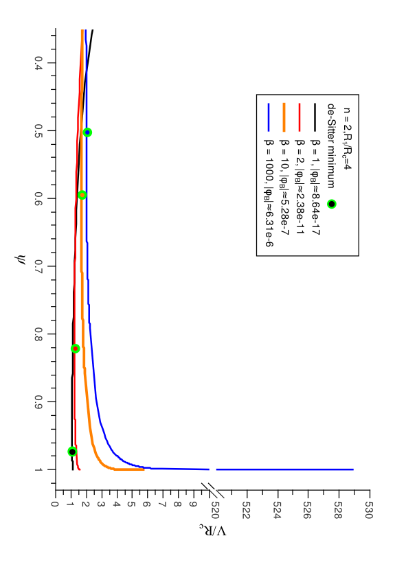

So far we have focussed on large limit of Starobinsky model as singularity is clearly avoided in this case. A comment on the finite behavior of the model is in order. In this case, the analysis requires numerical treatment. In Fig.3, we have displayed the parameter region consistent with local gravity constraints in case of finite values of and . In agreement with Ref.[24], we find that the local gravity constraints are satisfied provided that , see Fig.3. Furthermore, in gravity, the power spectrum acquires an additional slope [11] which is constrained in Ref. [25]. As demonstrated by Starobinsky , should satisfy the constraint, . Thus the model proposed in Ref.[21], with , violates this constraint too. If we adhere to observational constraints imposed by local gravity constraints, the model is vulnerable to curvature singularity. It is really interesting that the height of the barrier between de-Sitter minimum and curvature singularity turns out to be proportional to which is heavily constrained by local gravity constraints. In what follows, we shall address this issue.
III Finite time generic singularity and its reconciliation
Let us note that in the limit of , and the maximum of the potential is located at whose magnitude is given by
| (40) |
Since and , we find that . The minimum of the potential in free space given by (40) can be estimated numerically, at . In this case the height of the potential barrier for large value of is approximately equal to as shown in the Fig.2. The local gravity constraints impose a restriction on the height of the barrier or equivalently, the parameter for a given value of and . In case of , and , the model passes both the local gravity constraints. For large values of , the height of the potential barrier becomes large thereby hiding the singularity but resulting into clear violation of local gravity constraints. We also observe that taking small values of , the de-Sitter minimum shifts towards singularity, see Fig.2. This implies that we should have moderate values of parameters for a viable evolution. Situation gets worse when we move to high density regime whose treatment requires extreme fine tuning of initial conditions of the field[20].
As we have seen that the size of for any viable gravity and is constrained to be less than . This means that the minimum of the potential corresponding to , is very close to even in the case of baryonic/dark matter density.
It should be emphasized that in case of large curvature, the quantum effects become important leading to higher curvature corrections. Keeping this in mind, we can incorporate term in the model under consideration[11, 15](see Ref.[26] on the similar theme) which allows us to move the singularity away from . The Big Bang nucleosynthesis constraint at MeV ( or tells us that the correction term should satisfy the following condition[27],
| (41) |
If we choose , we find that . In case of neutron star with , the parameter is constrained to be . The local gravity constraints are satisfied in this case as
| (42) |
Let us note that in case we intend to describe inflation with the help of terms a la Starobinsky model, the numerical value of is much smaller than the quoted value. Indeed, the mass of scalaron (), if it is to be inflaton, should be [11] which implies that is much smaller than its numerical value quoted in case of neutron star. Such a correction does not disturb the neutron star physics and nucleosynthesis constraint but can help in avoiding the curvature singularity. As a result, the correction term can not contribute any effect to the local gravity experiments. This implies that the behavior of the model improves in the high curvature regime though it might be quite challenging to probe it numerically.

We can see from Fig.(4) that in case the BBN condition on is satisfied, the model would have a standard matter phase. Then a small is not only necessary for the BBN but also for the matter phase. Furthermore because of this additional term the curve cross the line for a finite while for the HSS model. Thus we can connect the early phase of accelerated expansion to the late time acceleration of universe without a singularity of the curvature scalar .
IV Conclusions
In this paper we have examined the variants of HSS models described by three parameters, , and [21]. The HSS scenario in Starobinsky parametrization corresponds to and . These models can satisfy the local gravity constraints and have potential capability of being distinguished from cosmological constant. The de-Sitter minimum of the effective potential of the scalar degree of freedom is quite close to curvature singularity for moderate values of and in these models. For larger values of and , the de-Sitter minimum moves towards singularity. The potential barrier between the de-Sitter minimum and curvature singularity is finite in HSS models which makes them delicate. Thus one should carefully tune the scalaron evolution such that it does not hit singularity while evolving in the neighborhood of the minimum of effective potential. For a given value of , the height of the barrier is defined by the parameter which is large for larger values of thereby hiding the singularity behind the potential barrier[21]. However, large potential barrier between singularity and de-Sitter minimum comes into conflict with the local gravity constraints.
The high curvature behavior of is extremely crucial for local gravity constraints to be evaded. In case slowly as it happens in case of large , we can not satisfy the local gravity constraints. On the contrary, if approaches zero fast, the corresponding models become more vulnerable to singularity as the minimum of the effective potential moves very near to singularity in the high curvature regime. In this case, the models under consideration can hardly be distinguished from cosmological constant.
The HSS scenario is build very carefully such that the curvature dependence of is just right to satisfy the local gravity constraints and at the same time to allow to distinguish itself from . Thus the finite time singularity in viable models is generic. However, the safe passage of the scalaron to the minimum of its effective potential can be ensured by the appropriate fine tuning of the scalaron evolution[20]. The fine tuning turns ugly in case of compact objects like neutron stars. The introduction of higher curvature terms becomes legitimate near singularity and can in principle improve the behavior of the model. The resulting scenario can give rise to a viable cosmic evolution.
V Acknowledgements
We are indebted to A. Starobinsky for taking pain in reading through the first draft of the manuscript and making important suggestions for its improvement. We also thank L. Amendolla and I. Waga for useful discussions. RG thanks the Centre for Theoretical Physics, Jamia Millia Islamia, New Delhi for hospitality. IT is supported by ICCR fellowship. MS is supported by ICTP through its associateship program.
References
- [1] V. Sahni and A. A. Starobinsky, Int. J. Mod. Phys. D9, 373 (2000) [arXiv:astro-ph/9904398].
- [2]
V. Sahni and A. A. Starobinsky, Int. J. Mod. Phys. D15, 2105 (2006) [arXiv:astro-ph/0610026];
T. Padmanabhan, AIP Conf. Proc. 861, 179 (2006) [arXiv:astro-ph/0603114];
P. J. E. Peebles and B. Ratra, Rev. Mod. Phys. 75, 559 (2003); L. Perivolaropoulos, arXiv:astro-ph/0601014;
N. Straumann, arXiv:gr-qc/0311083; J. Frieman, AIP Conf. Proc. 1057, 87 (2008) [arXiv:0904.1832];
M. Sami, Lect. Notes Phys.72, 219 (2007); M. Sami, arXiv:0901.0756 . - [3] E. J. Copeland, M. Sami and S. Tsujikawa, Int. J. Mod. Phys. D15 , 1753 (2006) [arXiv:hep-th/0603057].
- [4] E. V. Linder, Rept. Prog. Phys. 71, 056901 (2008) [arXiv:0801.2968].
- [5] R. R. Caldwell and M. Kamionkowski, arXiv:0903.0866.
- [6] A. Silvestri and M. Trodden, arXiv:0904.0024.
- [7] J. Frieman, M. Turner and D. Huterer, Ann. Rev. Astron. Astrophys. 46, 385 (2008) [arXiv:0803.0982].
- [8]
S. Weinberg, Rev. Mod. Phys. 61, 1 (1989);
S. M. Carroll, Living Rev. Rel. 4, 1 (2001) [arXiv:astro-ph/0004075];
T. Padmanabhan, Phys. Rept. 380, 235 (2003) [arXiv:hep-th/0212290]; R. Bousso, Gen. Rel. Grav. 40, 607 (2008) [arXiv:0708.4231]. - [9]
S. Capozziello, Int. J. Mod. Phys. D11, 483 (2002) [arXiv:gr-qc/0201033];
S. Capozziello, S. Carloni, and A. Troisi
Recent. Res. Dev. Astron. Astrophys. 1, 625 (2003) [arXiv:astro-ph/0303041];
S. Carroll, V. Duvvuri, M. Trodden and M. S. Turner, Phys. Rev. D70, 043528 (2004) [arXiv:astro-ph/0306438];
T. P. Sotiriou and V. Faraoni [arXiv:0805.1726];
S. Nojiri and S. Odintsov, Gen. Rel. Grav. 36, 1765 (2004) [arXiv:hep-th/0308176]. - [10] Wayne Hu and I. Sawicki, Phys. Rev. D76, 064004 (2007) [arXiv:0705.1158].
- [11] A. A. Starobinsky, JETP. Lett. 86, 157 (2007), [arXiv:0706.2041].
- [12] S. A. Appleby and R. A. Battye, Phys. Lett. B654, 7 (2007) [arXiv:0705.3199].
- [13] S. A. Appleby and R. A. Battye, JCAP 0805, 019 (2008) [arXiv:0803.1081].
- [14] A. V. Frolov, Phys. Rev. Lett. 101, 061103 (2008) [arXiv:0803.2500].
- [15] Abha Dev , D. Jain , S. Jhingan , S. Nojiri , M. Sami and I. Thongkool, Phys. Rev. D78, 083515 (2008) [arXiv:0807.3445].
- [16] T. Kobayashi and K. Maeda, Phys. Rev. D78, 064019 (2008) [arXiv:0807.2503].
- [17] T. Kobayashi and K. Maeda, Phys. Rev. D79, 024009 (2009) [arXiv:0810.5664].
- [18] S. Nojiri and S. D. Odintsov, arXiv:0903.5231; S Nojiri and S D Odintsov, arXiv.0804.3519; K. Bamba, S Nojiri and S D Odintsov, arXiv:0807.2575; S capozziello, M De Laurentis, S Nojiri and S D Odintsov, arXiv:0903.2753.
- [19] E. Babichev and D. Langlois, arXiv:0904.1382.
- [20] A. Upadhye and Wayne Hu, arXiv:0905.4055.
- [21] V. Miranda, S. E. Joras, I. Waga and M. Quartin, arXiv:0905.1941.
- [22] J. Khoury and A. Weltman, Phys. Rev. Lett. 93, 171104 (2004) [arXiv:astro-ph/0309300]; Phys. Rev. D69, 044026 (2004) [arXiv:astro-ph/0309411].
- [23] L. Amendola, R. Gannouji, D. Polarski and S. Tsujikawa, Phys. Rev.D75, 083504 (2007) [arXiv:gr-qc/0612180].
- [24] S. Capozziello and S. Tsujikawa, Phys. Rev. D77, 107501 (2008) [arXiv:0712.2268].
- [25] M. Tegmark, D. Eisenstein, M. Strauss et al., Phys. Rev. D74, 123507 (2006) [arXiv:astro-ph/0608632].
- [26] M. Abdalla, S. Nojiri and S. D. Odintsov, Class. Quant. Grav. 22, L35 (2005) [arXiv:hep-th/0409177].
- [27] P. Zhang, Phys. Rev.D76, 024007 (2007) [arXiv:astro-ph/0701662].