Magnetic dynamics with spin transfer torques near the Curie temperature
Abstract
We use atomistic stochastic Landau-Lifshitz-Slonczewski simulations to study the interaction between large thermal fluctuations and spin transfer torques in the magnetic layers of spin valves. At temperatures near the Curie temperature , spin currents measurably change the size of the magnetization (i.e. there is a longitudinal spin transfer effect). The change in magnetization of the free magnetic layer in a spin valve modifies the temperature dependence of the applied field-applied current phase diagram for temperatures near . These atomistic simulations can be accurately described by a Landau-Lifshitz-Bloch + Slonczewski equation, which is a thermally averaged mean field theory. Both the simulation and the mean field theory show that a longitudinal spin transfer effect can be a substantial fraction of the magnetization close to .
I Introduction
Spin transfer torque describes the interaction between the spin of itinerant, current-carrying electrons and the spins of the equilibrium electrons which comprise the magnetization of a ferromagnet. This torque results from the spin-dependent exchange-correlation electron-electron interaction, and leads to the mutual precession of equilibrium and non-equilibrium spins around the total spin. In spin valves with sufficiently high current density, spin transfer torque can excite a free ferromagnetic layer to irreversibly switch between two stable configurations (typically along an easy-axis, parallel or anti-parallel to an applied magnetic field), or to undergo microwave oscillations. Previous considerations of spin transfer torque mostly focus on the transverse response of the magnetization to spin currents [1, 2, 3, 4]. This is appropriate since the temperatures used in spin valve experiments are substantially below the Curie temperature of the ferromagnets, so that longitudinal fluctuations can be ignored. Near , one expects an interplay between the large thermal fluctuations and the nonequilibrium spin transfer torque. Generally speaking, theories of critical phenomena in out-of-equilibrium systems have only recently been developed [5, 6], and there remain many open questions on this topic.
Even far from the Curie temperature, temperature plays an important role in quantitatively analyzing the dependence of the magnetic orientation on the applied field and applied current. The effect of finite temperature on spin dynamics in the presence of spin transfer torque has been modeled the macrospin approximation (fixed magnetization length) by adding a Slonczewski torque to the Langevin equation describing the stochastic spin dynamics [7, 8], and by solving the Fokker-Planck equation with the spin transfer torque term added to the deterministic dynamics [9]. The Keldysh formalism provides a formal derivation of the stochastic equation of motion [10] for the non-equilibrium (i.e., current-carrying) system for a single spin of fixed magnitude. These treatments successfully describe the thermal characteristics of nanomagnets under the action of spin torques, such as dwell times and other details of thermally activated switching.
For materials like GaMnAs, experiments are done near , so that the size of the magnetization is substantially reduced from its zero temperature value (temperature in Kelvin), and undergoes sizeable fluctuations. In this case, the applicability of a macrospin model is not clear. For field-driven dynamics, there is theoretical work which accounts for longitudinal fluctuations near [11]. This formal treatment culminates in the construction of the Landau-Lifshitz-Bloch equation (LLB), which is an extension of the familiar Landau-Lifshitz equation with an additional longitudinal degree of freedom. In this work, we consider temperatures near the Curie temperature and include both longitudinal fluctuations of the magnetization and the influence of spin transfer torque.
There are a number of issues that complicate magnetic dynamics near , including the temperature dependence of more basic magnetic properties such as magnetic damping and magneto-crystalline anisotropy, as well as the temperature dependence of the spin transfer torque itself. We use an atomistic approach for the stochastic dynamics of a local moment ferromagnet with the inclusion of spin transfer torque. Such a model is more appropriate for systems like the dilute magnetic semiconductor GaMnAs. Our use of simple approximations for the temperature dependence of the magnetic anisotropy, demagnetization field, and damping allow us to focus in the interplay between thermal fluctuations and spin transfer torque. We find that within this model, spin currents can change the size of the magnetization. We give an expression for this “spin-current longitudinal susceptibility”, and propose an experimental scheme to measure this effect.
We construct a Landau-Lifshitz-Bloch + Slonczewski (LLBS) equation to describe both longitudinal fluctuations and spin transfer torques. Following Ref. 12, we verify the applicability of the LLBS equation by comparing its results to the atomistic results. We then analyze the LLBS equation to find the applied field-applied current phase diagram for different temperatures. We find that critical switching currents are reduced by the same mechanism exploited in heat assisted magnetic recording, namely the temperature-induced reduction in the magnetic anisotropy [13]. We also find that regions of the phase diagram which have been experimentally unattainable become relevant at high temperatures. The dependence of critical currents on temperature in these regions can provide quantitative details about the temperature dependence of spin transfer torque.
II Method
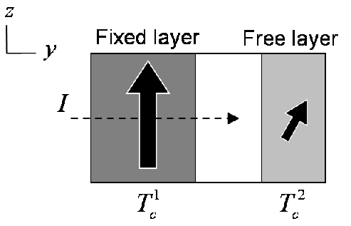
To study the interplay between temperature and spin transfer torque, we consider a spin valve with a fixed layer magnetization in the -direction with Curie temperature , and a free layer with a smaller Curie temperature (see Fig. (1)). This allows for a nearly temperature independent spin current flux incident on the free layer. We make the approximation that all of the incoming spin current is absorbed uniformly throughout the free layer magnetization. This approximation is based on two expectations. Substantial spatial and temporal inhomogeneities in the magnetization should induce rather irregular spatial patterns in the spin currents carried by propagating states. This will lead to large dephasing effects, so that the total spin current should rapidly decay away from the interface as in the conventional picture of spin transfer torques[3]. In addition, in this temperature regime, and for thin layers (), magnetic non-uniformities in the direction transverse to current flow should be more substantial than non-uniformities along the current flow resulting from a localized spin transfer torque.
II.1 Stochastic Landau-Lifshitz with spin transfer
We adopt three approaches to model the system. The first is an atomistic lattice model of normalized spins , which results in a stochastic Landau-Lifshitz equation (SLL). We include nearest-neighbor Heisenberg coupling with exchange constant , and an easy-axis anisotropy field of magnitude in the -direction. To model the temperature dependence of the anisotropy, we make the ansatz that the magnitude of anisotropy at temperature is proportional to the reduced magnetization :
| (1) |
so that the anisotropy field on spin is given by , where the bar indicates a spatial average. A hard-axis anisotropy field with magnitude in the -direction is added to model the demagnetization field of the thin layer. We make an ansatz for the form of this field to make the numerics more tractable. We take the demagnetization field to be uniform on all spins and given by . This form of the hard-axis field ensures that , and roughly captures the non-local nature of the field. Finally, we include an applied field in the -direction. The Hamiltonian for spin is then:
| (2) | |||||
where the sum in the first term is over nearest neighbors, is the Bohr magneton, and is the permeability of free space. To model nonzero temperatures, we add damping and a stochastic field to the equation of motion implied by Eq. (2), with the standard statistical properties:
| (3) | |||||
| (4) |
where are the Cartesian components of the field, is the Boltzmann constant, is the magnetic moment on each lattice site, and is the gyromagnetic ratio. We numerically integrate the equation of motion using a second-order Heun scheme [14]. We add a Slonczewski-like spin transfer torque term to the equation of motion for the th spin, which is given finally as:
| (5) | |||||
parameterizes the spin transfer torque: , where is the applied current, is the spin polarization of the current, is the zero temperature magnetization, is the free layer thickness, is the transverse layer area, and is the electron charge. The effective magnetic field is given by . We use both a bulk geometry consisting of a periodic array of spins in 3 dimensions (simple cubic lattice), and a layer geometry with an array of 100 100 15 spins. We employ the bulk geometry in comparing the stochastic model behavior with predictions from mean field theory, and the layer geometry for studying the effect of spin current on magnetization size.
II.2 Landau-Lifshitz-Bloch + Slonczewski equation
In the second approach, we add a Slonczewski torque term to the LLB equation. To derive the LLB equation, a probability distribution for the spin orientation is assumed, which is used to find the ensemble average of Eq. (5). In addition, the nearest neighbor exchange field is replaced by its mean-field value. The details of the derivation follow closely those in Ref. 11, so we omit them here. The final LLB+Slonczewski equation takes the form:
| (6) | |||||
with an effective field given by:
| (7) | |||||
where is the zero temperature saturation magnetization, is the dimensionless magnetization with magnitude between zero and one, is the zero field, zero current equilibrium magnetization: , and is the Brillouin function. is the longitudinal susceptibility: . is the 0th component of the Fourier transformed exchange, and is a vector with size between 0 and 1. The spin transfer torque is parameterized by , as described in the previous section. The double cross product in Eq. (6) is the familiar Landau-Lifshitz damping term, which describes the relaxation of the magnetization direction to the nearest energy minimum. The term longitudinal to distinguishes the LLB equation from the Landau-Lifshitz equation. This longitudinal term describes the relaxation of the size of the magnetization to its steady state value, which is determined by the temperature, applied fields, and applied currents.
The detailed dependence of the magnetic anisotropy on temperature is generally material specific. In our model, the anisotropy and demagnetization fields depend on temperature through their dependence, and vary as and , respectively. The magnetic exchange can also depend on temperature. This dependence is stronger for ferromagnets with indirect exchange interactions (such as GaMnAs, where the magnetic interactions are mediated by hole carriers), and weaker for local moment systems with direct exchange (such as Fe). For simplicity we treat as temperature-independent.
Finally we consider the standard Landau-Lifshitz equation with a reduced but fixed saturation magnetization. We find in Sec. (III.4) that it is possible to appropriately modify the damping coefficient in a standard Landau-Lifshitz approach so that the phase diagram it predicts agrees qualitatively with those predicted by the more complicated models.
III Results
III.1 Longitudinal spin current susceptibility
In transition metal ferromagnets, longitudinal spin transfer, which is another way of saying spin accumulation, is typically quite small compared to the magnetization and has a negligible effect on the magnetization dynamics. However, for temperatures close to the Curie temperatures, the longitudinal spin transfer can be a sizeable fraction of the magnetization and can significantly affect the dynamics.
Using the LLB+Slonczewski equation, it is straightforward to show that the change in the magnetization in the presence of spin current is
| (8) |
This longitudinal spin transfer effect is demonstrated in Fig. 2, which shows the longitudinal susceptibility to magnetic field and spin current for a full stochastic simulation with 10010015 spins. (In the figure, is rescaled: the magnetic field is scaled by the exchange field , and the magnetization is scaled by .) In the simulation, the spins’ polar angle is initialized to a uniform distribution between and , where is chosen so that the initial spins’ average is equal to the equilibrium value. We allow the system to relax to steady state, and find the value of the magnetization and its fluctuations by finding the average and standard deviation over an interval of time (the appropriate time interval is temperature dependent). The fluctuations lead to the statistical uncertainty shown in Fig. (2).
The spin current susceptibility is defined as . We find that and correspond very well, demonstrating that Eq. (8) accurately describes the numerical stochastic model.
The change in magnetization should be measurable. The fractional change in the magnetization compared to the zero-temperature saturation magnetization is
| (9) |
For , so that (from Fig. (2)), and with an exchange field of (which corresponds to a of 150 K in a cubic nearest neighbor Heisenberg model), , , , , and gives a change compared to the zero temperature value of 5 %. Since the magnetization is reduced to approximately 20 % of its zero temperature value at , the fractional change in the magnetization is approximately 25 %.

A notable aspect of this longitudinal spin transfer is that the size of the magnetization can either be increased or decreased according to the direction of current flow. For electron flow from fixed to free layer, the free layer moment increases, while electron flow in the opposite direction decreases the free layer moment. This contrasts with current-induced Joule heating, which always decreases the magnetization.
This distinction can be exploited to probe the longitudinal spin transfer by using the experimental scheme shown in Fig. (3). We consider the case where . We choose sign conventions such that a positive aligns with the fixed layer, and a positive current represents electron flow from fixed to free layer. In the absence of a longitudinal spin transfer (=0, black line in Fig. (3)), the application of a magnetic field will partially order the free layer to align or anti-align with the fixed layer. This should cause the resistance of the device to change in some way, according to the giant magnetoresistance effect and magnetic order induced in the free layer (the detailed dependence of on is not important here). If a positive current is applied, then the longitudinal spin transfer induces partial ordering of the free layer, so that . Then the curve of , and therefore the curve is simply shifted by (the red dashed curve in Fig. (3)). If a negative current density is applied, then and the and curves are shifted by (black dotted curve in Fig. (3)). This shift represents a unique signature of longitudinal spin transfer.
Using the same parameters as before, we estimate a total shift between for positive and negative current to be on the order of . Eq. (9) indicates that materials with small exchange field (or small ), and those that can support large current densities show the effect most strongly. This suggests that weak metallic ferromagnets such as , and Fe alloys such as and [15] may be good candidates for free layer material.

III.2 Landau-Lifshitz-Bloch-Slonczewski vs Stochastic Landau-Lifshitz
In this section, we compare the results obtained from the full 3-dimensional stochastic LL+S equation with those obtained from the mean-field LLBS equation. In our numerics, we rescale time to as , which rescales the magnetic fields by the exchange field . Dimensionless fields are denoted by lowercase: , etc. The dimensionless spin torque is denoted by , where . We consider a current-induced magnetic excitation for the bulk lattice geometry at various temperatures. The average magnetization is initialized at a angle with respect to the -direction (the individual spins’ initial direction is distributed uniformly within in the direction about ). The spin transfer torque is applied to excite the magnetization away from the -direction. The parameters used are an applied field of , a demagnetization field of , a current of , and damping of (the artificially high damping was chosen to allow the numerical simulation of the switching to be carried out in a reasonable time). The time step used for the numerical integration is . We vary the temperature , and present results in terms of the scaled temperature .
As we increase temperature, we obtain trajectories of varying complexity. Fig. (4) compares the LLBS and several realizations of the stochastic Landau-Lifshitz equation. For this range of parameters, the magnetic dynamics evolves from steady oscillations to current induced switching as the temperature is increased. Generally, the level of correspondence between the two is qualitatively good, although it varies between different realizations of the stochastic dynamics. We can conclude from this data that the LLBS equation qualitatively captures the features of the full stochastic simulations.
The trajectories for indicate that a realization of stochastic dynamics can exhibit the crossover from precession to stable switching, whereas at this temperature the trajectory obtained with the LLBS equation shows only oscillations. This illustrates an important distinction between the stochastic Landau-Lifshitz and LLBS models. The LLBS is an equation for the thermally averaged magnetization, derived using an assumed probability distribution function (in this case, a distribution function most appropriate for temperatures well above and below energy barriers). For this reason, the LLBS does not contain information about fluctuations, and in particular does not capture stochastic switching over the energy barrier. The fluctuations may be obtained by solving the Fokker-Planck equation, or by supplementing the LLBS equation with stochastic fields, as done in Ref. 16.

III.3 Applied field-applied current phase diagram
Both high temperatures and the longitudinal degree of freedom change the applied field-applied current phase diagram of the free magnetic layer. Fig. (5) shows the generic topology for regions of stability for the parallel (“P”, or -direction) and antiparallel (“AP”, or -direction) fixed points. We focus on the stability of the AP configuration for positive applied fields (the dashed boundary in the upper-half-plane of Fig. (5). We first briefly describe the main qualitative features before providing a mathematical description. For applied fields between and , the stability boundary is a horizontal parabola, while for other values of applied field, the stability boundary is linear with slope . For applied fields with magnitude less than , there is hysteresis in the current switching. For , this phase diagram reduces to the known form found experimentally [17]. As increases, the size of the hysteretic region (and the switching current) decreases. Also the range of field with the parabolic boundary decreases, and the outer edge of the parabola gets pulled in closer to 0. For sufficiently high temperatures, this parabolic stability boundary should be experimentally accessible.
A quantitative description of the phase diagram follows from Eq. (6). We determine the stability of fixed points using the standard method of linearizing Eq. (6) about a fixed point and finding parameter-dependent eigenvalues . A positive real part of indicates a loss of stability. This analysis leads to the following condition for instability of the antiparallel configuration (where it should be noted that depends on through , and is the rescaled susceptibility, given by ):
This leads to a cubic equation for . Assuming , and expanding to 0th order in leads to an approximate, closed form for . Again we distinguish between different regimes of applied field. For
| (10) |
where again is the equilibrium magnetization in the absence of applied field and applied current. Eq. (10) shows that the slope of the boundary is temperature independent, and is given by (the intrinsic damping is assumed to be temperature independent). The temperature independence of the slope follows from the fact that the spin transfer torque increases like , but the effective damping rate also increases as . The intercepts of this boundary line are temperature dependent due to the temperature dependence of . The contribution from the easy-axis anisotropy field has an additional temperature dependence, but the magnitude of this field is much smaller than the demagnetization field, so it does not play an important role. The critical current at zero field is reduced by because of the reduction in the demagnetization field. This is important because the demagnetization field is usually larger than applied fields, and is therefore the primary impediment to current induced switching. Its reduction through increased temperature offers a route to reduced critical switching currents.
For , a very large spin torque is required to stabilize the AP configuration. The values of current for which the AP configuration is stabilized are much higher than those attainable experimentally, so that for this range of fields the AP configuration is not seen [18]. The approximate critical current along the AP stability boundary is:
| (11) |
The reduction in the outer boundary of the parabolic stability line is reduced at high temperature, and this reduction can also be traced back to the reduced magnetic anisotropy. For low temperatures, the application of spin transfer torques results in a elliptical precession mostly in the easy plane about the fixed point. To stabilize the AP configuration in this regime, the spin transfer torque must overcome the precessional torque (usually, the spin transfer torque must overcome the much weaker damping torque). Assuming for definiteness, the precessional torque decreases with as , while the spin transfer torque increases like . This implies a value for the maximum reach of the parabola of . Plugging in typical values for material parameters (the same used in Sec. (III.1)) leads to a critical current of for . This is an order of magnitude smaller than the zero temperature case. The behavior of this critical current versus temperature at a fixed applied field is shown in Fig. (6). (Solid line gives LLBS result). It should also be noted that the stochastic trajectories (shown in Fig. (4)) indicate that thermal fluctuations can effectively drive the system out of the precessional state and into the static antiparallel configuration.

III.4 Comparison with Landau-Lifshitz-Slonczewski
The Landau-Lifshitz-Slonczewski (LLS) equation can be modified to emulate the LLBS equation. Based on the qualitative behavior of the LLBS equation, a suitable form for a temperature dependent LLS equation for a nanomagnet of reduced magnetization size and orientation is:
where , and the temperature dependence is contained entirely in . Clearly the divergence of the damping at is unphysical, however a more detailed treatment of damping near is beyond the scope of this paper. The differences between this LLS equation and the LLBS equation are quantitative (as opposed to qualitative) in nature. One difference is in the dependence of the critical current on temperature for . Fig. (6) shows the prediction based on the LLS equation.

The LLS equation equation neglects the longitudinal spin transfer and applied field susceptibility, which are responsible for dynamically changing the size of the magnetization (and therefore the size of the effect fields) during a switching event, or other magnetization dynamics. However, Fig. (6) shows qualitative agreement between the critical currents found in both LLBS and LLS models. This is indicative of the fact that for the applied field-applied current phase diagram, the spin-current and applied-field longitudinal susceptibilities play a role that is secondary to the more pronounced effects of temperature reduced anisotropies.
IV Discussion
Spin transfer torques can affect the longitudinal fluctuations of a ferromagnet near its critical temperature. To consider these effects, we studied an atomistic, stochastic Landau-Lifshitz-Slonczewski simulation at high temperatures. We find that there is a longitudinal spin transfer effect, and estimate that at temperatures near , spin currents can measurably change the size of the magnetization. We then supplemented the Landau-Lifshitz-Bloch equation with a Slonczewski torque term, and verified that this model captures the qualitative features of the stochastic simulations. We showed that the applied field-applied current phase diagram undergoes large changes in the presence of high temperatures, and that these changes may be useful for reducing critical switching currents and for studying the detailed behavior of the temperature dependence of the spin transfer torque. It should be emphasized that these results are predicated on a disordered local moment model of a ferromagnetic phase transition. This model leads to an effective damping that increases with temperature as , which effectively counteracts the similar increase in the magnitude of spin transfer torque. Materials that undergo a Stoner transition should also have a dependence for the spin transfer torque, but a different temperature dependence for damping. Such materials should therefore behave differently than the model considered here.
The experimental system relevant for the effects we describe (shown schematically in Fig. (1)) should be relatively straightforward to fabricate. Jiang et al. considered a similar system [19], although that work dealt with other issues such as the ferrimagnet compensation point for magnetization and total angular momentum. By considering simpler ferromagnets with different Curie temperatures, the role of temperature may be more easily inferred. It is of course necessary to account for Joule heating in assessing the detailed temperature dependence of the spin transfer torque. However recent experiments on domain wall motion illustrates the feasibility of compensating for this effect [20]. On the other hand, experiments conducted at fixed current with varying ambient temperatures and applied fields may offer a more straightforward route to observing the longitudinal spin transfer effect.
Many experiments done with dilute magnetic semiconductors deal with domain wall motion, where thermal effects play an important role in even the qualitative aspects of the domain wall behavior[20]. There are additional challenges associated with extending this work from spin valves to continuous magnetic textures. Among these is the renormalization of the exchange interaction associated with the coarse graining of the magnetization, which becomes more important at higher temperatures [21]. In addition, the crucial role played by the demagnetization field in intrinsic domain wall pinning implies that the finite temperature treatment of the demagnetization field must also be handled more carefully. For these reasons the spin valve geometry may provide greater experimental control and admit a simpler theoretical description.
References
- [1] J. C. Slonczewski, J. Magn. Magn. Mat. 62, 123 (1996).
- [2] L. Berger, Phys. Rev. B 54, 9353 (1996).
- [3] M. D. Stiles and A. Zangwill, Phys. Rev. B 66, 014407 (2002).
- [4] A. Brataas, G. E. W. Bauer, and P. J. Kelly, Phys. Rep. 427, 157 (2006).
- [5] A. Mitra, S. Takei, Yong Baek Kim, and A. J. Millis, Phys. Rev. Lett. 97, 236808 (2006).
- [6] D. E. Feldman, Phys. Rev. Lett. 95, 177201 (2005).
- [7] Z. Li and S. Zhang, Phys. Rev. B 69, 134416 (2004).
- [8] J. Xiao, A. Zangwill, and M. D. Stiles, Phys. Rev. B 72, 014446 (2005).
- [9] D. M. Apalkov and P. B. Visscher, Phys. Rev. B 72, 180405 (2005).
- [10] A. S. Núñez and R. A. Duine, Phys. Rev. B 77, 054401 (2008).
- [11] D. A. Garanin, Phys. Rev. B 55, 3050 (1997).
- [12] O. Chubykalo-Fesenko, U. Nowak, R. W. Chantrell, and D. Garanin. Phys. Rev. B 74, 094436 (2006).
- [13] R. E. Rottmayer et al., IEEE Trans. Magn. 42, 2417 (2006).
- [14] J. L. Garcia-Palacios and F. J. Lazaro, Phys. Rev. B 58, 14937 (1998).
- [15] R. M. Bozorth, Ferromagnetism, D. Van Nostrand Company, New York (1951).
- [16] D. Garanin and O. Chubykalo-Fesenko, Phys. Rev. B 70, 212409 (2004).
- [17] S. I. Kiselev, J. C. Sankey, I. N. Krivorotov, N. C. Emley, R. J. Schoelkopf, R. A. Buhrman, and D. C. Ralph, Nature 425, 380 (2003).
- [18] Ya. B. Bazaliy, B. A. Jones, and S.-C. Zhang, Phys. Rev. B 69, 094421 (2002).
- [19] X. Jiang, L. Gao, J. Z. Sun, and S. S. P. Parkin, Phys. Rev. Lett. 97, 217202 (2006).
- [20] M. Yamanouchi, D. Chiba, F. Matsukura, T. Dietl, and H.Ohno, Phys. Rev. Lett. 96, 106601 (2006).
- [21] G. Grinstein and R. H. Koch, Phys. Rev. Lett. 90, 207201 (2003).