Quantum control and entanglement in a chemical compass
Abstract
The radical pair mechanism is one of the two main hypotheses to explain the navigability of animals in weak magnetic fields, enabling e.g. birds to see the Earth’s magnetic field. It also plays an essential role in the field of spin chemistry. Here, we show how quantum control can be used to either enhance or reduce the performance of such a chemical compass, providing a new route to further study the radical pair mechanism and its applications. We study the role of quantum entanglement in this mechanism, and demonstrate intriguing connections between radical-pair entanglement and the magnetic field sensitivity of the compass. Beyond their immediate application to the radical pair mechanism, these results also demonstrate how state-of-the-art quantum technologies could potentially be used to probe and control biological functions.
Introduction.— It is known that many species, including birds, insects and mammals, use the Earth’s magnetic field for orientation and navigation[1]. To explain this remarkable ability, two main hypotheses have been proposed: a magnetite-based mechanism and a radical pair biochemical reaction mechanism[1]. Since the radical pair mechanism (RPM) was first proposed in pioneering work by Schulten et al. [2], a chemical compass model for migratory birds, based on such a mechanism [3] has been widely studied. Evidence suggests that the RPM is indeed linked to the avian magnetoreception [5, 4]. It was recently demonstrated in spin chemistry experiments that a photochemical reaction can act as a compass even in a magnetic field as weak as the geomagnetic field [6]. The underlying mechanism in such a chemical compass is clearly of quantum mechanical nature. However, the detailed role of quantum interactions, in giving rise to entanglement and (de-)coherence, are little understood [7]. On the other hand, one can observe growing interest in the role of quantum coherence for biological processes in general [8], and specifically in photosynthesis [9]. A deeper understanding of the role of quantum mechanics in biology will eventually come along with the ability to control biological processes at the level of individual molecules. In physics, various kinds of quantum control techniques have been developed, specifically in the field of quantum information processing and quantum metrology [10, 11]. The question thus naturally arises to what extent these or similar techniques could be applied to test and refine certain biophysical hypotheses, such as the chemical compass model for animal magnetoreception? Can we use quantum technologies that have primarily been developed to control man-made microscopic systems, to study the behavior of living things — e.g. birds, fruit flies, or plants — in a detectable way?
In our work, aiming at the above questions, we will revisit the RPM and the chemical compass model using concepts and techniques from quantum information. The RPM can serve both as a magnetometer or as a compass, depending on the molecular realization. For simplicity, we will refer to both cases as “compass” in the following. First, we demonstrate that quantum control ideas can be applied to experiments in spin chemistry and potentially also to study the magnetoreception of certain animals. We propose several quantum control protocols that can be used to either enhance or suppress the function of a chemical compass. Assuming that the model provides the correct explanation for magnetoreception of certain species, we predict that they would loose or regain their orientability in appropriately designed experiments using such quantum control protocols – given that such experiments could be carried out safely. Our calculations show that the RPM can not only detect weak magnetic fields, but it is also sensitive to quantum control even without the presence of a static magnetic field. These results offer a new means to study experimentally the RPM, also in comparison with other conceivable mechanisms such as those in man-made magnetometers [12, 13].
Second, we investigate whether entanglement is a necessary ingredient in animal magneto-reception, which seems appealing in the light of the important role this concept has gained in fundamental discussions on quantum mechanics and its wider implications. As the sensitivity of the chemical compass depends on the initial state of the radical pair, it is natural to ask whether it needs to be quantum mechanically entangled – thereby excluding any conceivable classical mechanism – or whether classical correlations would be sufficient. We find that the answer largely depends on the radical pair lifetime. For specific realizations of the RPM, e.g. those in recent spin-chemistry experiments [14], entanglement features prominently and can even serve as a signature of the underlying spin dynamics. However, when the radical pair lifetime is extremely long, as it is believed to be the case in the molecular candidate for magneto reception in European robins [15, 16], entanglement does not seem to play a significant role.
Radical Pair Mechanism.— We consider a photochemical reaction that starts from the light activation of a photoreceptor, followed by an electron transfer process; two unpaired electrons in a spin-correlated electronic singlet state are then carried by a radical pair. The effective environment of a radical pair mainly consists of their individual surrounding nuclei. The Hamiltonian of a radical pair is of the form [17]
| (1) |
where is the electron gyromagnetic ratio, denote the hyperfine coupling tensors and , are the electron and nuclear spin operators respectively.
The initial state of a radical pair is assumed to be the singlet state , which subsequently suffers from de-coherence through the hyperfine interactions with the environmental nuclear spins. The initial state of the nuclear spins at room temperature can be approximated as , where is the dimension of the th nuclear spin. The charge recombination of the radical pair goes through different channels, depending on the electron-spin state (singlet or triplet). In particular, the yield of products formed by the reaction of singlet radical pairs can be calculated as [17]
| (2) |
where is the radical re-encounter probability distribution, and is the fidelity between the electron spin state at time and the singlet state. The ultimate activation yield in cryptochrome is believed to affect the visual function of animals [3].
We have followed the established theory for the dynamics of the RPM [18, 17] and computed the full quantum dynamics of the combined system of electron spins and nuclear spins. Technically, we employ the Chebyshev polynomial expansion method [19] to numerically calculate the exact evolution operator , and thereby all relevant physical quantities. We first consider the well-studied photochemical reaction of pyrene (Py-) and N,N-dimethylaniline (DMA-) [18], for which the hyperfine couplings are isotropic [14], and the tensor in (1) simplifies to a number . We study the role of entanglement in this radical pair reaction and propose new experiments based on quantum control. We then generalize our results to the cryptochrome radical pair of FADH∙-O, which is the molecular candidate believed to be involved in avian magnetoreception [15, 16]. We thereby show that our protocols work also for anisotropic hyperfine interactions, which are essential for direction sensitivity of the magnetic field [3].
Magnetic Field Sensitivity under Quantum Control.— The magnetic-field sensitivity of the radical pair reaction [Py- DMA-] is quantified by the derivative of the activation yield with respect to the magnetic field strength [14], i.e.
| (3) |
We assume that the external magnetic field points in the direction. The key ingredient in the RPM are the hyperfine interactions, which induce a singlet-triplet inter-conversion (mixing) depending on the magnetic field [17]. Using an exponential model as an example for the re-encounter probability distribution [17], we plot in Fig. 1(a) the magnetic-field sensitivity as a function of . Our numerical simulation agrees well with the experimental results in [14].
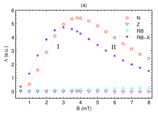

Studying the performance of the radical-pair mechanism under quantum control would allow us to test the role of entanglement and further details of the RPM in spin chemistry experiments. As a simple example, consider a periodical pulse sequence with -pulses applied at times along the direction; the effective Hamiltonian to the first order is given by . Such kind of control can actually enhance the performance of quantum-coherence based magnetometers, see e.g. [12, 13]. However, in case of the RPM, the magnetic-field sensitivity becomes greatly suppressed, as can be seen in Fig. 1(a). We can show that, whenever one applies more general decoupling protocols to promote quantum coherence in a radical pair reaction, its magnetic-field sensitivity will generally be reduced [20]. This demonstrates that it is in fact the decay of coherence, i.e. de-coherence, rather than coherence itself, that plays an essential role for the magnetic-field detection in RPM, different from the situation in magnetometers using e.g. NV-centers in diamond [13, 12].
To demonstrate a potentially positive effect of quantum control on a chemical compass, we consider a situation where the magnetic field alternates its direction periodically at times which will disturb the proper functioning of compass. (This situation is reminiscent of an experiment with birds in an oscillating field [5], even though the cause of the compass disfunction is here different.) If we now apply -X pulses at the same times , the chemical compass will recover its function as the transitions between and induced by the residual hyperfine interactions are still affected by the magnetic field [see Fig. 1(a)].
Entanglement and Magnetic Field Sensitivity.— We have hitherto assumed, as is usually done, that the radical pair starts in a perfect singlet state, i.e. that quantum coherence is fully maintained during the pair creation. In reality, the initial state of radical pairs will never be a perfect singlet (i.e. pure state), but a mixed state with a certain singlet fidelity . It is known that the value of has to be sufficiently close to unity, otherwise the state may also be described by classical correlations. We therefore ask: Is entanglement, as a genuine quantum signature, needed at all to account for the efficiency of the magnetic compass? Or could the latter be explained by mere classical correlations? To answer this question, we have randomly chosen different initial states from the set of separable states and calculated the maximal achievable magnetic field sensitivity for every value of , see Fig. 1(b) (). We find that, in the operating region of the compass (around mT), the maximal achievable sensitivity for separable states stays significantly below the sensitivity for the singlet state, and this maximum sensitivity is in fact attained by the classical mixture . In turn, if nature is allowed to optimize the initial state from the full set of states, including the entangled states (e.g. and , see Fig. 1(b)), the optimum magnetic-field sensitivity will typically be much higher than for any separable state. On these grounds one can say that entanglement is indeed helpful, and it is specifically entanglement rather than mere quantum coherence.
To test experimentally whether the initial state of the radical pair is indeed (close to) a singlet state, i.e. whether de-coherence can be neglected during the radical pair creation, one could apply a -X pulse as the reaction starts. For an initial singlet state, which remains invariant under such pulse, the magnetic field sensitivity will remain unchanged, whereas for an initial classical mixture it will collapse, see Fig. 1(b).
As entanglement seemingly plays a role in the RPM with Py-DMA, we have studied its dynamics and its quantitative connection to the magnetic-field sensitivity. Similar to the activation yield, we define to quantify the effective amount of entanglement that is present in the active radical pairs during the reaction, where is chosen to be the entanglement measure of concurrence [21] at time . The first derivative with respect to the magnetic field, , quantifies how sensitive this effective entanglement is with respect to variations of the magnetic field.


In Fig. 2(a), we see that and are correlated in the regions of I and II, displaying monotonic relations with different linear ratios. This result is remarkable insofar as that the time during which entanglement exists is significantly shorter than the reaction time for the value of to saturate [20]. However, it can also be seen from Fig. 2(a) that changes dramatically at the crossover between regions I and II. This step-like behavior relates to the discontinuity of the entanglement lifetime as the magnetic field increases, see Fig. 2(b). In the region of I, is much shorter than the reaction time , while it jumps to a larger value comparable with during the crossover from the region of I to II. When we further increase the magnetic field, exhibits more kinks but with less increment. This effect originates from the finite size of the nuclear spin bath [22] of the electron spins, and is a clear signature of the system-environment dynamics underlying the RPM [20].
Applications to Animal Magnetoreception.— In order to account for a direction sensitivity of the singlet yield, which is necessary for compass function, the hyperfine couplings must be anisotropic [3]. Here we consider an example of such a radical pair, FADH∙-O, which was proposed as a likely molecular candidate underlying the magnetoreception of European robins [15, 16], but it may also play this role in other species.


The direction of the magnetic field in (1) with respect to the reference frame of the immobilized radical pair is described by two angles , i.e. . Without loss of the essential physics, we here assume that , and investigate the dependence of the singlet yield on the angle when we apply quantum control. First, it can be seen from Fig. 3 (a) that the angular dependence of the singlet yield is much suppressed if one applies -pulses along the same direction as the magnetic field, which can distinguish the RPM from other potential mechanisms for magnetoreception [12, 13]. Next, we study the scenario that the magnetic field changes it direction periodically at times as in the previous section. As expected, the angular dependence is again greatly suppressed, as can be seen from the lower curve in Fig. 3(b). However, if one applies -pulses perpendicular to the direction of the magnetic field this will re-induce an angular dependence, see Fig. 3(b). Furthermore, we find that even without a static magnetic field, quantum control can induce an angular dependence of the singlet yield as shown in Fig. 4. In other words, if one would be able to design a behavior experiment with animals that use a chemical compass to sense the magnetic field, in such an environment they would lose or regain their orientability, depending on the applied control fields. This would provide further evidence for the RPM as the underlying mechanism, and it could help to narrow down the possible candidates of radical pairs in animal magnetoreception. It is however not clear how such experiments could be carried out safely.

Different from the example of Py-DMA we find that here the entanglement only exists in a time range ( ns) that is much shorter than the expected radical pair lifetime (s). We would thus not expect entanglement to play a significant role in this context. To check this further, we have computed the achievable sensitivity of the compass for different initial states and found that a substantial part of all separable states can account for an angular dependence that is as high as (or even higher) than for the singlet state [20]. This means that – in contrast to Py-DMA – the radical-pair entanglement does not seem to be a necessary ingredient for a chemical compass based on FADH∙-O.
Summary and Outlook.— We have demonstrated how quantum control can influence radical pair reactions and the function of a chemical compass. The presented protocols can in principle be applied to existing spin chemistry experiments, even though the implementation of coherent spin control [23, 24] in this context needs to be further developed. They might also provide a route for future experiments with biological systems (including animals or plants) that are expected to exploit the RPM; in this case a much more careful study would be required, in particular regards the potential side effects of short control pulses on biological tissue.
We found interesting connections between entanglement and the magnetic field sensitivity when the radical pair lifetime is not too long compared to the coherence time. Otherwise, the role of coherence and entanglement seem to be insignificant. Whether or not birds or other animals use entanglement for their ability to orient themselves in the earth magnetic field remains an open question, whose answer will depend on the specific molecular realization of their chemical compass.
As a bio-mimetic application of practical relevance, it would be interesting to explore the possibility of simulating a radical-pair mechanism in more controllable quantum systems, such as NV centers in diamond [12, 13, 25], to design an ultra-high fidelity sensor for the detection of weak fields or forces.
Acknowledgements.— We are grateful for the support from the FWF (Lise Meitner Program, SFB FoQuS).
References
- [1] R. Wiltschko and W. Wiltschko, Bioessays 28, 157 (2006); S. Johnsen and K. J. Lohmann, Nature Rev. Neurosci 6, 703 (2005); C. T. Rodgers and P. J. Hore, Proc. Natl. Acad. Sci 106, 353 (2009).
- [2] K. Schulten, C. E. Swenberg and A. Weller, Z. Phys. Chem NF111, 1 (1978).
- [3] T. Ritz, S. Adem and K. Schulten, Biophys. J 78, 707 (2000).
- [4] W. Wiltschko and R. Wiltschko, J. Exp. Biol 204, 3295 (2001).
- [5] T. Ritz et. al, Nature 429, 177 (2004).
- [6] K. Maeda et. al, Nature 453, 387 (2008).
- [7] Recent work even claims that the quantum Zeno effect is vital for avian magnetoreception: I. K. Kominis, Phys. Rev. E 80, 056115 (2009); see also J. A. Jones, P. J. Hore, Chem. Phys. Lett. 488, 90 (2010).
- [8] D. Abbott, P. C. W. Davies and A. K. Pati (eds.) Quantum Aspects of Life (World Scientific, Singapore, 2008);H. J. Briegel, S. Popescu, arXiv:0806.4552; S. Lloyd, Nature Physics 5, 164 (2009); W. H. Zurek, ibid. 5, 181 (2009); J. Gilmore and R. H. McKenzie, J. Phys. Chem. A 112, 2162 (2008).
- [9] G. S. Engel et. al, Nature 446, 782 (2007); H. Lee, Y.-C. Cheng and G. R. Fleming, Science 316, 1462(2007); M. Mohseni, P. Rebentrost, S. Lloyd and A. Aspuru-Guzik, J. Chem. Phys 129, 174106 (2008); M. B. Plenio and S. F. Huelga, New J. Phys 10, 113019 (2008).
- [10] L. Viola, E. Knill and S. Lloyd, Phys. Rev. Lett 82, 2417 (1999); R. de Sousa, N. Shenvi and K. B. Whaley, Phys. Rev. B 72, 045330 (2005); G. S. Uhrig, Phys. Rev. Lett 102, 120502 (2009).
- [11] H. G. Krojanski and D. Suter, Phys. Rev. Lett. 93, 090501 (2004); L. M. K. Vandersypen, I. L. Chuang, Rev. Mod. Phys. 76, 1037 (2005).
- [12] J. M. Taylor et. al., Nature Physics 4, 810 (2008).
- [13] J. R. Maze et al., Nature 455, 644 (2008).
- [14] C. T. Rodgers et al., J. Am. Chem. Soc 129, 6746 (2007).
- [15] T. Ritz et al., Biophys. J 96, 3451 (2009).
- [16] I. A. Solov’yov, K. Schulten, Biophys. J 96, 4804 (2009).
- [17] U. E. Steiner, T. Ulrich, Chem. Rev 89, 51 (1989).
- [18] H.-J. Werner, Z. Schulten, K. Schulten, J. of Chem. Phys, 67, 646 (1977).
- [19] V. V. Dobrovitski, H. A. De Raedt, Phys. Rev. E 67, 056702 (2003).
- [20] See Supplementary Material for further information.
- [21] W. K. Wootters, Phys. Rev. Lett 80, 2245 (1998).
- [22] N. V. Prokofev, P. C. E. Stamp, Rep. Prog. Phys 63, 669 (2000).
- [23] J. Berezovsky et al., Science 320, 349 (2008).
- [24] G. D. Fuchs et al., Science 326, 1520 (2009).
- [25] G. Balasubramanian, et al., Nature 455, 648 (2008).
Supplementary Material
This is supporting material for our paper. We derive the completely
positive map for the dynamics of a central spin coupled to its
surrounding nuclear spins with isotropic hyperfine interactions, and
use it to investigate the evolution of entanglement in the radical
pair reaction. To identify the role of entanglement in the radical
pair mechanism, we randomly choose the initial state from the set of
separable states, to compute the optimum magnetic field sensitivity
for these states and compare it with the sensitivity for an inital
singlet state. Further details are provided to clarify the
connections between quantum entanglement and magnetic field
sensitivity. To illustrate the essential role of the (de-phasing)
nuclear spin environment in a chemical compass, we investigate a
hypothetical reference model of bosonic thermal bath and compare it
with the present results.
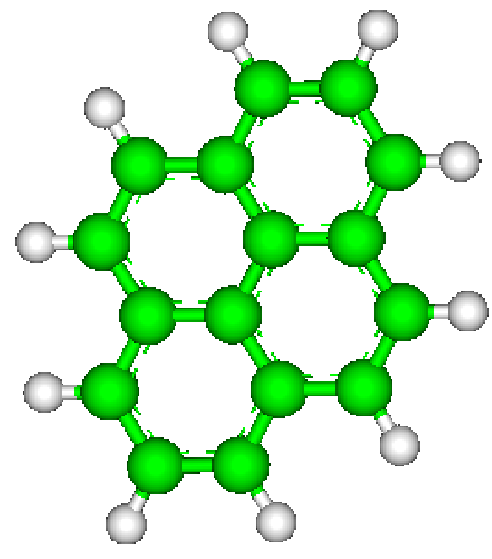
Molecular structures of radical pairs.— The molecular structures for the radical pair Py-DMA are displayed in Fig. 1, Py- has ten spin- hydrogen nuclei, while the DMA- has eleven spin- hydrogen nuclei and one spin- nitrogen nucleus; the nuclear spin of carbon is . In our numerical simulations, without loss of essential features, we have considered three groups of equivalent nuclei in each radical that have the largest hyperfine couplings as in [1], i.e. the radical Py- interacts with ten spin- surrounding nuclei with the hyperfine coupling constants mT (4 H), mT (4H), mT (2H) [1], and the radical DMA- is dominantly coupled with seven spin- nuclei with mT (6H), mT (1H), and one spin- nucleus with mT (1 N), see Table 2 of [1].

The flavin radical FADH∙ is displayed in Fig. 2. We consider the dominant hyperfine couplings from two
spin- nitrogen nuclei and three spin- hydrogen
nuclei as in [2].
The superoxide radical O is devoid of the
hyperfine couplings, which is likely to lead to higher sensitivity
against weak magnetic fields [3, 4].

Completely positive map for electron spin dynamics.— We here derive the completely positive map for the case of isotropic hyperfine interaction. The Hamiltonian for a central unpaired electron spin coupled with a nuclear spin bath is written as
| (4) |
where . The presently available theories for the central spin problem usually resort to the perturbation approach, based on certain approximations, e.g. the quasi-static approximation or the limit of large magnetic fields and/or large spin bath polarizations. For our present purpose, these approximations are only of limited use since, in the radical pair mechanism, one is particularly interested in the region of low fields, and the number of most relevant surrounding nuclei is 10, in contrast with in quantum dots.
It is straightforward to show that the total angular momentum of the electron and nuclear spins, , where , is conserved for the Hamiltonian in Eq. (4), i.e. . By introducing as the basis of eigenstates of , i.e. , where labels the eigenvalues and is a degeneracy index, we can express the initial state of the spin bath as , where is the total dimension of all the (relevant) nuclear spins. Thus, under the coherent evolution , the joint state of the central spin and the nuclear spins evolves as
| (5) | |||||
| (6) |
wherein and denote the eigenstates of , and belongs to the eigenspace of associated to the eigenvalue . The fact that the total angular momentum is conserved results in orthogonality relations for the nuclear spin states:
| (7) |
The inner products of these vectors are zero, as they belong to orthogonal subspaces (or are null vectors). By recalling the notation , , , , we obtain
| (8) |
in which we have used the relation in Eq. (7). In a similar way, one can show that . Moreover, it is easy to verify that
Thus, the dynamics of the central spin, which is calculated by tracing out its spin bath degrees of freedom as , can be explicitly expressed as
from which we can obtain the completely positive map for the central
spin dynamics. If we rewrite the evolution operator
in the form of , we get the above
dynamic parameters , and
.
Dynamics of quantum entanglement in Py-DMA.— In Fig. 3, we plot the evolution of entanglement between two unpaired electron spins in the radical pair reaction [Py- DMA-]. We have used the concurrence [5] as the measure of two-spin entanglement, which vanishes on separable states and assumes its maximum value, 1, on maximally entangled states such as the singlet state. We also compare the exact value of entanglement with the estimated best lower bound of entanglement . The agreement between them is good (even though not perfect). This fact supports our statement about how one could possibly estimate the amount of entanglement from experimentally accessible information.

We also plot the dynamics of entanglement under X and Z
control in Fig. 3. It can be seen that entanglement
survives indeed for a longer time if quantum control is
applied.
Protecting coherence is not helpful.— In the quantum coherence based magnetometer, e.g. with NV centers in diamond [6, 7], the sensitivity is indeed dependent on the coherence time, i.e. the longer the coherent time is the better the sensitivity. In this section, we use the simple example of the radical pair with only isotropic hyperfine couplings to show that this is not the case in the present model.
As we have described in the main text, for the Z control, we dynamically decouple the xx and yy hyperfine interactions while keeping the magnetic-field dependent Zeeman interactions. Nevertheless, the magnetic field sensitivity is still much suppressed. This phenomenon can be understood as follows. The residual hyperfine couplings along the longitudinal direction (i.e. zz hyperfine couplings) only induce the transitions between the singlet state and one specific triplet state , while these two eigenstates are degenerate and their energies are independent of the magnetic field. In this case, the singlet-triplet interconversion is actually not influenced by the magnetic field, the effects of which are thus not detectable through the singlet yield. We will prove, in the following, that a chemical compass will loose its function, if one uses general dynamical decoupling protocols to promote the electron spin coherence.
Assume that, at time , the electron spins and the surrounding nuclear spins are in some state . The activation yield during a short time interval is
| (9) |
with the singlet fidelity . We then write its first derivative with respect to the magnetic field as
which obviously determines the ultimate magnetic field sensitivity as by summing up for all time intervals , . The singlet fidelity at time is with , and is the Hamiltonian of the electron spins together with the nuclear spins as in Eq. (L1) [8]. By using a perturbation expansions for small , we have
| (10) |
which enables us to express the singlet fidelity as follows,
| (11) |
where . Using the properties of the singlet state that , where , the first derivative of can be written as
| (12) |
If , one can
easily
verify that . Thus, if a dynamical decoupling protocol is to protect
the electron spin coherence during the reaction, i.e. keep the spin
state close to the singlet state, we can conclude that , and will be of the fourth order in , which is an
order smaller than the one from other general states. We remark that
we do not trivially assume that the system dynamics is frozen by
protecting coherence, but the electron spin state does evolve even
if it is kept closer to the singlet state under decoupling
controls.


Magnetic field sensitivity from random separable or incoherent states.— Here we compare the magnetic field sensitivity obtained from an initial singlet state (entangled) with the sensitivity obtainable from classically correlated states (separable). A mixed quantum state is called separable if it can be written as a sum of product states
| (13) |
In general, a separable state can exhibit “coherence”, by which one means that some of its off-diagonal density matrix elements (with respect to the standard basis , ) are non-zero. By definition, however, a separable state is not entangled. So there is an essential difference between entanglement and coherence.
We introduce the optimal magnetic field sensitivity for the radical pair reaction [Py- DMA-] on the set of separable states as
| (14) |
where denotes the magnetic-field sensitivity for a given initial state . It can be proved that the optimal sensitivity is obtained by the product states . In our numerical calculations, we randomly choose product states and calculate . We also randomly choose the initial state from the set of incoherent states, the off-diagonal matrix elements of which are all zero, meaning that no coherence is present (and naturally no entanglement either). This is what we have done to compute the curve ‘Sep’ in Fig. L1(b). We find, somehow surprising, that the optimal sensitivity from the incoherent states is the same as . In this sense, quantum coherence is not vital for the magnetic-field sensitivity.
In the example of FADH∙-O, we characterize the angle dependence by using the quantity of visibility defined as follows
| (15) |
where is the singlet yield. We have randomly chosen a few
hundreds of product states and incoherent states as the initial
radical pair state, and calculated the corresponding visibility
(compared with the visibility for the singlet state). It can
be seen from Fig. 4 that a substantial part of separable
(incoherent) states can account for an angular dependence that is as
high as (or even higher) than for the singlet state. In this sense,
the radical pair initial state of an avian compass need not be the
singlet state.
Quantum entanglement and magnetic field sensitivity.— To quantify the amount of entanglement that exists in the active radical pairs during the reaction, similar to the singlet yield, we define the effective entanglement as the integral
| (16) |
Its first derivative with respect to the magnetic field is the entanglement sensitivity
| (17) |
In Fig. 5, we plot as a function of . It can be seen that changes conspicuously (kink) during the crossover between the regions of I and II. At the same time, the entanglement yield always increases with the magnetic field. This can be understood from the fact that strong magnetic fields will energetically suppress the relaxation (spin flips) in the longitudinal direction. By this process, the state of the electron pairs changes towards a binary mixture of two entangled states (namely and ), which is entangled for almost all values of the mixing parameter, resulting in a much longer lifetime of entanglement.


To further illustrate the connection between quantum entanglement and the magnetic field sensitivity, we plot in Fig. 5 the time evolution of the entanglement and of the value of the accumulated magnetic-field sensitivity , for different values of the magnetic field: mT, mT, mT, and mT. The lifetime of entanglement in the region of I is approximately ns, while needs about ns to reach its saturate value, see Fig. 6(a-b). We can also explicitly see the sudden increase of when crosses between the regions I (low magnetic field) and II (high magnetic field), from ns to about ns, see Fig. 6(c-d), which gives rise to the steps in Fig. L2 (b) [8].
At this point, it is worth to emphasize that the concept of
entanglement is different from the singlet fraction (fidelity),
which was studied earlier. Generally speaking, a state can exhibit
significant classical spin correlations without having any
entanglement. In our specific example, at any time during the
radical-pair reaction there will be a finite singlet fraction while
entanglement, in contrast, will only exist for a much shorter time
(as shown in Fig. 6). In this sense, entanglement is a
different, and generally more sensitive, signature than the singlet
fraction. See also Fig. L2(b) in the main text.
Reference model of a bosonic heat bath.— Let us assume that each of the unpaired electron spins is coupled with an independent bosonic heat bath at the same temperature. The dynamics of one central spin would thus be described by the following Lindblad type master equation [9, 10]
| (18) |
where , with , and . The solution of the above master equation can be represented by a map which is explicitly expressed as follows
where , and . This map describes spin-exchange interactions with the environment with an effective rate and an equilibrium parameter that is related to the environment temperature . The dependence of and on and the magnetic field is given in the following way: and , where depends on the system-bath coupling strength on resonance, and the bosonic distribution function is with the system energy scale and the thermal energy scale . Thus we have
| (19) | |||||
| (20) |
We are interested in the effects of low magnetic fields, for example mT, which corresponds to the thermal energy scale at temperature mK that is quite low for biochemical systems. Thus we can naturally assume that , from which it is easy to verify that , e.g. if K then is already four orders smaller than .
The radical pair starts in the singlet state , and its state evolves as . At time , the density matrix is of the following form
| (21) |
where , , , and . Thus we can calculate the singlet fidelity as
The activation yield for the exponential re-encounter probability model is , i.e.
One can verify that under the general conditions we are interested in, the magnitude of the magnetic field sensitivity would increase with the coupling strength scale , i.e. the fast thermalization is good in the present context. To achieve the optimal bound of and illustrate the essential physics, we can assume that is much larger than (this is different from the real situation where is smaller than ), which leads to
| (22) |
The magnitude of from the bosonic heat bath decreases as the temperature increases. Even at temperature as low as K, it is already significantly smaller than the one from the nuclear spin environment, see Fig. 7. Therefore, we can conclude that the effects of low magnetic fields will indeed be washed out completely by the thermal fluctuations.

By calculating , we find that will always grow as the magnetic field becomes stronger, as long as , which is obviously satisfied in the regions we are interested in. The change of the sign of happens at . At room temperature K, this would correspond to the magnetic field T.

The evolution of entanglement as obtained from Eq. (21) is . In a similar way, one can obtain the lifetime of entanglement, see Fig. 8, which is monotonically increasing with the magnetic field. This is another feature in marked contrast with the nuclear spin environment: there are no oscillatory kinks in the entanglement lifetime as the magnetic field increases.
References
- [1] Rodgers, C. T., Norman, S. A., Henbest, K. B., Timmel, C. R. and Hore, P. J. Determination of radical re-encounter probability distributions from magnetic field effects on reaction yields. J. Am. Chem. Soc 129, 6746 (2007).
- [2] Cintolesi, F., Ritz, T. , Kay, C. W. M. , Timmel, C. R., Hore, P. J. Anisotropic recombination of an immobilized photoinduced radical pair in a 50-T magnetic field: a model avian photomagnetoreceptor. Chem. Phys. 294, 385 (2003).
- [3] Timmel, C. R., Till, U., Brocklehurst, B., McLauchlan, K. A. and Hore, P. J. Effects of weak magnetic fields on free radical recombination reactions. Molecular Physics 95, 71-89 (1998).
- [4] Ritz, T., Wiltschko, R., Hore, P. J., Rodgers, C. T., Stapput, K., Thalau, P., Timmel, C. R. and Wiltschko, W. Magnetic Compass of Birds Is Based on a Molecule with Optimal Directional Sensitivity. Biophys. J 96, 3451 (2009).
- [5] Wootters, W. K. Entanglement of formation of an arbitrary state of two qubits. Phys. Rev. Lett 80, 2245 (1998).
- [6] Taylor, J. M., Cappellaro, P., Childress, L., Jiang, L., Budker, D., Hemmer, P. R., Yacoby, A., Walsworth, R. and Lukin, M. D. High-sensitivity diamond magnetometer with nanoscale resolution. Nature Physics 4, 810 - 816 (2008).
- [7] Maze J. R. et al. Nanoscale magnetic sensing with an individual electronic spin in diamond. Nature 455, 644-647 (2008).
- [8] References to equations and figures in the Letter start with an “L”, i.e. “Eq. (L3)” means “Eq. (3) in the Letter”.
- [9] H. P. Breuer, F. Petruccione,The Theory of Open Quantum Systems (Oxford Univerity Press, New York, 2002).
- [10] Briegel, H. J. and Englert, B. G. Quantum optical master equations: The use of damping bases. Phys. Rev. A 47, 3311-3329 (1993).