Non-Abelian Vortices at Weak and Strong Coupling in Mass Deformed ABJM Theory
Abstract:
We find half-BPS vortex solitons, at both weak and strong coupling, in the supersymmetric mass deformation of ABJM theory with gauge symmetry and Chern-Simons level . The strong coupling gravity dual is obtained by performing a quotient of the supersymmetric eleven dimensional supergravity background of Lin, Lunin and Maldacena corresponding to the mass deformed M2-brane theory. At weak coupling, the BPS vortices preserving six supersymmetries are found in the Higgs vacuum of the theory where the gauge symmetry is broken to . The classical vortex solitons break a colour-flavour locked global symmetry resulting in non-Abelian internal orientational moduli and a moduli space of solutions. At strong coupling and large , upon reduction to type IIA strings, the vortex moduli space and its action are computed by a probe D0-brane in the dual geometry. The mass of the D0-brane matches the classical vortex mass. However, the gravity picture exhibits a six dimensional moduli space of solutions, a section of which can be identified as the we find classically, along with a Dirac monopole connection of strength . It is likely that the extra four dimensions in the moduli space are an artifact of the strong coupling limit and of the supergravity approximation.
1 Introduction
The study of vortices with non-Abelian, internal orientational degrees of freedom, has revealed beautiful connections between their moduli space dynamics and features of the gauge theory they live in [1, 2, 3, 4]. Typically, such classical solutions occur when the non-Abelian gauge symmetry is spontaneously broken, and crucially, there exists a “colour-flavour locked” global symmetry in the vacuum. A vortex solution breaking this colour-flavour symmetry then gives rise to a continuous family of classical solutions which proves to be useful in extracting vortex dynamics in the moduli space approximation. In this paper we will investigate Chern-Simons vortex solitons in 2+1 dimensions, carrying non-Abelian internal orientational zero modes. The theory we consider is a mass deformation of the supersymmetric ABJM theory [5] preserving all supersymmetries [6].
Vortex solitons in Abelian and non-Abelian Chern-Simons theories have been widely studied in both relativistic and non-relativistic settings [7, 8, 9, 10, 11, 12]. Detailed reviews of these can be found in [13, 14]. More recently, the moduli space dynamics of (supersymmetric) non-Abelian Chern-Simons vortex solitons with internal collective coordinates, was analyzed in [15, 16, 17, 18]. It was already noted in [19] that the Chern-Simons action induces terms which are first order in time derivatives in the moduli space effective description of the vortex. Specifically, the authors of [16, 17] demonstrated that the effect of the Chern-Simons coupling on the moduli space quantum mechanics of SUSY non-Abelian vortices, is to induce a coupling to a magnetic field which could then be given a geometric interpretation in terms of the first Chern character of an index bundle over the moduli space.
One of our main motivations is to study the semiclassical, solitonic objects arising in the context of the recently discovered superconformal ABJM theory [5] in 2+1 dimensions. The theory has a gauge symmetry with matter in the bifundamental representation and a level Chern-Simons action for the gauge fields. It describes the world-volume dynamics of multiple M2-branes moving in a orbifold background in M-theory. The ABJM proposal followed the seminal works of Bagger-Lambert [20] and Gustavsson [21] (BLG), which first proposed the superconformal theory on multiple M2-branes probing flat space.
We will see that the ABJM theory, when deformed by a particular supersymmetric mass term, admits finite energy, non-Abelian Chern-Simons vortex solitons. What makes the situation particularly interesting is that the soliton dynamics can now be explored in two different regimes of the field theory: one in which semiclassical analysis is valid and another wherein the theory is strongly coupled and is described by a dual gravitational background. The study of vortices in these two regimes, including the construction of the classical solution and obtaining the dual gravity description at strong coupling, will be the subject of the paper. Using these two approaches we confirm the general picture of [16, 17], while also encountering certain unresolved puzzles.
Various nonperturbative objects have been found in BLG and ABJM theories. Monopole instantons in ABJM theory have been studied in [22]. Vortex solitons have been already studied in mass deformed BLG theory in [23, 24]. The solution found in [23] has a topological winding and a mass that is twice the one found in [24]. Vortices in mass deformed ABJM have been studied in [25]; those solutions can be interpreted as higher winding solutions with respect to the ones that we will study in this paper. Vortices in the non-relativistic limit of ABJM have been studied in [26].
Both the BLG theory in 2+1 dimensions and the ABJM theory admit mass deformations breaking conformal invariance, but preserving all of their supersymmetries [27, 28, 29, 30, 6]. In particular, the maximally supersymmetric mass deformation of the ABJM theory was obtained in [6, 30] and the analysis of its classical vacuum structure revealed a discrete set of vacua [6]11 1 A potential discrepancy was also noted, since the classical vacuum states of the mass deformed theory are more numerous than expected from the supergravity dual.. This deformation breaks the global symmetry of the ABJM theory to .
We focus our attention on one of these classical vacua which we expect to be perturbatively accessible for large (and ), and we refer to this vacuum as the “Higgs vacuum”. Here the gauge group is broken to . We find that this vacuum admits classical vortex solutions carrying both electric and magnetic charge. Importantly, the Higgs vacuum exhibits a global symmetry, where the second factor arises via a combination of (broken) flavour rotations and global gauge transformations. This colour-flavour locked transformation acts non-trivially on our vortex solution which breaks to , resulting in a moduli space of solutions. We are able to construct the classical solutions for all , and show that they have finite energy and that they are BPS. We explicitly check that the solutions are invariant under six supercharges and are -BPS states with a mass given by , where is the mass deformation parameter of the theory.
The topology of the vacuum manifold in the Higgs vacuum is non-trivial, , and the vortex solitons carry a charge. However, they are actually stabilized also by a global charge which is quantized to be a multiple of [5], and which is not carried by the perturbative states in the theory. Thus an -vortex state cannot annihilate into the vacuum. Although the vortex solution is straightforward to obtain, its low energy dynamics on the moduli space appears technically challenging to derive from first principles. On general grounds, at weak coupling, since the solutions preserve six supersymmetries and the moduli space of solutions we have found is an , we expect the moduli space dynamics to be governed by supersymmetric quantum mechanics on a sphere. However this leaves unclear, the effect of the Chern-Simons terms on this quantum mechanics.
To learn more about the soliton dynamics we turn to the other parametric regime where the mass deformed ABJM theory is tractable. This is the strongly coupled, large limit, namely , with large. In this limit the superconformal ABJM theory is dual to eleven dimensional supergravity on obtained by a particular quotient of the solution dual to the superconformal theory. We deduce the gravity dual of the mass deformed ABJM theory by performing a similar quotient on the background dual to the maximally supersymmetric mass deformation of the superconformal M2-brane theory. The latter background, preserving SUSY, and symmetry, was obtained in [27, 29]. In the fermion fluid language of Lin, Lunin and Maldacena [29], the vacua of the , theory are in one to one correspondence with partitions of and are represented by states of free fermions. The Higgs vacuum is the trivial partition and is a highly excited particle state in the fermion picture. This can be interpreted as the geometry generated by a dielectric M5-brane carrying units of M2-brane charge and wrapped on one of the two ’s in the invariant geometry.
The quotienting of the background above, by the action, yields the Higgs vacuum of the mass deformed ABJM theory, preserving an symmetry. For large (such that is fixed and large), we can reduce the geometry to type IIA string theory. The type IIA geometry asymptotes to and contains two spheres and , each associated to one of the two factors of the isometry group. The Higgs vacuum corresponds to a dielectric D4-brane wrapping [31]. The presence of the dielectric D4-brane can also be directly inferred from a fuzzy sphere interpretation of the classical VEVs in the Higgs vacuum [32]. The general picture bears a strong resemblance to the theory [33, 34, 35], although the geometries in the present situation are completely non-singular. Non-Abelian vortices in the theory where studied in [36, 37].
The vortex soliton in the Higgs vacuum is a D0-brane probe in the above geometry22 2 In the D-brane picture, the dielectric D4-brane will have a -field along its worldvolume directions. This allows a D0-brane to form a bound state with the D4, corresponding to a noncommutative U(1) instanton in 5 dimensions, and appear as a vortex in the non-compact 2+1 dimensions.. Surprisingly, we find that the probe mass is minimized along a six dimensional submanifold , preserving the reduced set of isometries. The value of the probe mass along the moduli space matches the value deduced classically. The probe moduli space can be viewed as fibred along a segment , where the is also non-trivially fibred over the two ’s. The topology of a section at a generic point of the segment is . At the two tips of , the three-sphere shrinks to zero 33 3 We thank D. Tong for drawing our attention to this. and the section is given by a two-sphere. We identify the tip where the obtained by fibering over shrinks as the moduli space of vortex solutions we saw at weak coupling. The probe dynamics in this section of is that of a particle on of radius coupled to a Dirac monopole connection of strength . The radius of the sphere also matches that of the fuzzy sphere from the classical analysis of the Higgs vacuum. The effect of the Chern-Simons interactions on the moduli space of the soliton, is to induce a Dirac monopole connection. This picture is in agreement with the general results of [16, 17]. However, the full six dimensional moduli space at strong coupling presents a puzzle, and does not appear to have a simple interpretation in terms of the soliton solutions we found at weak coupling.
The paper is organized as follows. In Section 2, we review the essential features of the ABJM theory and its mass deformation, their symmetries, vacuum structure and equations of motion. Importantly, we describe the origin of the colour-flavour locked symmetry in the Higgs vacuum. In Section 3, we present our ansatz for the vortex soliton solutions for general and discuss their stability and verify explictly that they are left invariant by six supersymmetries. In Section 4, we turn to the gravity dual of the mass deformed ABJM theory. We first review the basic features of the symmetric solution of [27, 29] and then explain the quotienting procedure that yields the mass deformed ABJM theory. The D0-brane probe dynamics and its moduli space are then deduced straightforwardly. We summarize our results and conclusions in Section 5. In Appendix A the vortex fermionic zero modes are discussed for .
Note Added: While this paper was being completed, a closely related preprint arXiv:0905.1759 [hep-th] [38] appeared, which overlaps with our classical field theory analysis of the vortex solitons.
2 Mass deformed ABJM theory
The bosonic part of the Lagrangian of the ABJM theory [5] is given by a Chern-Simons theory, coupled to bifundamental matter with a scalar potential. The Chern-Simons levels associated to the two gauge groups are and respectively. In superspace notation the ABJM superpotential for the bifundamental matter fields reads
| (1) |
where and transform in the representation of the gauge group. The global R-symmetry becomes explicit upon introducing the fields
| (2) |
and the bosonic part of the ABJM Lagrangian becomes
| (3) | |||||
which is manifestly invariant under the R-symmetry associated to supersymmetry. The covariant derivatives on the bifundamental fields are defined as
| (4) |
The fermionic part of the Lagrangian is,
| (5) | |||||
The conventions for -matrices are as in [39]:
| (6) |
To raise and lower spinor indices the symbol is used, with . The charge conjugation on spinors is given by . The metric choice is
In [6], a mass deformation of the ABJM theory was found which preserves all the supersymmetries and breaks the global symmetry down to . The action swaps the matter fields and , while the factors act individually on the doublets and respectively. The symmetry rotates with a phase and with a phase . This perturbation can be written as a superpotential in the superfield formalism discussed in [30]. The R-symmetry group is . This mass deformed theory is an example of three dimensional supersymmetric theory with the so called ”non-central” term in the supersymmetry algebra [40, 41] ; this means that the anticommutator of the supercharges closes not only in a combination of momentum generators and central charges, but also in generators of the R-symmetry. The expression in component fields is:
| (7) | |||||
where . The scalar potential of the mass deformed theory can be written in a compact way as
| (8) |
where
It is also possible to consider the theory with gauge group . In this case for we recover the Bagger-Lambert theory [20]. The global symmetry of the theory, is given by the baryon number (under which have charge ).
In the gauge theory the naive baryon number symmetry is gauged by a gauge field corresponding to the off-diagonal combination of the two Abelian factors in . The remaining Abelian symmetry acts trivially on all the matter fields and couples to the theory through the Abelian Chern-Simons interaction . Hence there is another global symmetry generated by the current which is related by the the equation of motion for to the current,
| (9) |
The flux quantization condition on implies that the charges are quantized as integer multiples of . In the ABJM theory, the chiral primary operators made from elementary fields, of the form , do not carry this charge. Gauge invariant operators carrying the quantized baryon number correspond to combinations of the form along with ’t Hooft operators. The presence of this global charge under which elementary states are uncharged will be important for the stability of the vortex solitons we find in the mass deformed theory below.
2.1 Vacua and symmetries
After mass deformation, the ABJM theory has several isolated classical vacua preserving different amounts of gauge symmetry. These were obtained in [6]. As in the case of the theory in dimensions [33, 34], classical vacua may be enumerated by finding block diagonal solutions to the F-term vacuum conditions. In this case, for the scalar potential to vanish we must have
| (10) |
These equations have simple solutions if we assume that either or . In the following we will concentrate on some configurations with . This choice breaks the discrete symmetry. The potential for such configurations is
| (11) |
We consider the following vacuum, which corresponds to an irreducible solution and we will call this the Higgs vacuum,
In this vacuum the gauge symmetry is almost completely broken by the VEV,
| (23) |
It is a trivial fact that the factor cannot be broken, because it couples to the other fields of the theory just through Chern-Simons interactions. If we label the two different gauge groups as and , the Higgs vacuum configuration breaks and the . The unbroken gauge symmetry is a particular combination of the with a diagonal generator of the gauge group which acts on from the left. All other generators of are broken. The unbroken generator is
| (24) |
The global symmetry acting on the doublet is also broken.
Similar to the case of the theory, the above solutions can be interpreted as fuzzy complex coordinates, which can be decomposed into real (Hermitian) coordinates as in [39],
| (25) |
The Higgs vacuum configuration implies that
| (26) |
which formally resembles a fuzzy equation. However, due to the fact that is Hermitian implying that , one suspects that the configuration actually describes a fuzzy two sphere. This latter picture has been confirmed in [32]. Qualitatively the situation is somewhat similar to the Higgs vacuum of the theory characterized by such a fuzzy sphere configuration which breaks both a global flavour symmetry and the gauge group. There, a combination of the broken gauge and flavour generators can be shown to generate a “colour-flavour” locked symmetry [36, 37] which leaves the VEVs invariant.
One expects therefore that the Higgs vacuum of the mass deformed ABJM theory should have an unbroken global symmetry which is a combination of the broken gauge transformations and the broken global symmetry that acts on the doublet . Indeed, we find such a colour-flavour locked global symmetry of the vacuum.
For every , there is a special combination of the broken global symmetry and of the broken gauge symmetry which is left unbroken by the VEV. Let us first denote the three generators of in an irreducible representation of dimension , as (with )
Now consider the following global transformation , acting on the :
| (27) |
It can be checked that such a global transformation of the VEVs can be undone by embedding the global rotation into (constant) gauge transformations:
| (28) |
where
Note that it is only the broken gauge transformations which are involved in the colour rotation. We denote this unbroken “colour-flavour” locked symmetry as . Thus the Higgs vaccum of the mass deformed ABJM theory has this symmetry and excitations around this vacuum should fall into multiplets of the symmetry. A nice explanation of how this embedding of global rotations in the gauge group is made possible, is given in [32] 44 4 As explained in [32], the set of matrices are generators of . If we further define , it is easily checked that these satisfy commutation relations. The transform as adjoints of the gauge symmetry and provide an -dimensional irreducible representation of the algebra. One may do the same with the matrices and define . These furnish an dimensional irreducible representation and are adjoints under the gauge symmetry. The action of these generators of the gauge symmetry on the bifundamentals precisely matches a global rotation. . We will be interested in vortex solitons in this vacuum and the existence of the colour-flavour locked symmetry has interesting implications for the solitons.
2.2 Equations of motion
The classical picture for the vacuum states of the theory above and the classical solutions we now look for, will only be valid in the weakly coupled regime which in turn implies . Since the ABJM theory has no Maxwell terms for the gauge fields, the equations of motion for the gauge field yield Gauss law type constraints. These are of the form
| (32) | |||
where the field strength is defined as:
| (33) |
Finally there are the second order equations of motion for the scalar fields , with the ansatz ,
| (34) | |||||
where
| (35) |
The equation of motion for is identical to this and and can be obtained from the above by exchanging all ’s with ’s.
We will look for static, axially symmetric solutions to the above equations of motion carrying charge under the symmetry generated by . To this end we set the time derivatives of and to zero where are polar coordinates on the plane. In addition we choose the gauge . We then get the following constraints between and which are particularly useful in solving for the scalar potentials, since they are only algebraic conditions on the latter,
| (36) | |||
These relate the non-Abelian charge densities to the magnetic flux carried by the configuration, in each gauge group factor. In our vortex ansatz we can use this constraint to fix the form of once that we have fixed an ansatz for and for . Note that this is a first order equation, but determines algebraically. The second set of Gauss constraints relate to , yielding a second order differential equation. In addition to this we also need to ensure that the conditions (and ) emerging as a consequence of azimuthal symmetry are consistently satisfied.
Once we obtain explicit solutions to the Lagrange equations of motion, we can compute the mass of the soliton using the following expression for the energy density
| (37) |
3 Vortex in the Higgs vacuum
Let us first of all discuss the topology of the vacuum manifold
| (38) |
There is a subtlety in the definition of that we now need to note. One combination of the centers of the and acts non-trivially on the matter fields and this action can be undone by a rotation in . The other combination results in a centersymmetry under which the matter fields are uncharged. Due to this reason, the fundamental group of is given by , where the factor corresponds to non-contractible loops around which fields wind by a rotation generated by the diagonal combination of the centers of the and factors. We can then write the homotopy exact sequence:
From a straightforward application of the properties of the homotopy exact sequence, it follows that
| (39) |
The vortex solitons are classified by a topological quantum number; if we take a configuration made of elementary vortices, they are not in principle any more topologically stable.
From the topological point of view, a configuration made by vortices actually corresponds to a trivial element of . However, there is another quantum number that can make the -vortex configuration stable. As we have explained above, in the gauge theory, the perturbative states of the theory are not charged under the global symmetry defined by the current in Eq. (9). The vortex solitons we find will be charged under this symmetry and for this reason protected from decaying to the perturbative states. The charge carried by these vortices is measured by the magnetic flux associated to , carried by the soliton. These vortex solitons can also be thought of as states created by the ’t Hooft monopole operators in the Higgs vacuum of the mass deformed theory. See [43] for a discussion of the corresponding operators in conformal field theories.
In this section we will write an explicit ansatz for the elementary vortex in the theory. The vortex solutions in the theory can be obtained by simply projecting out the abelian part from the gauge fields .
3.1 Vortex Solution for
We begin with the simplest example with . In this case the solution that we find is very similar to the one found in [24] in the mass-deformed Bagger-Lambert-Gustavsson theory, which, for corresponds to ABJM theory with gauge group [44]. The vortex ansatz should be axially symmetric in two dimensions and the scalar field VEVs should asymptote to the Higgs vacuum. We therefore take the ansatz,
| (40) |
where the second scalar winds around origin. The ansatz breaks completely, the gauge symmetry which acts from the right. A combination of the diagonal generator of with is however, preserved, while all fields are neutral under . The vacuum manifold
| (41) |
has the fundamental homotopy group, . However, as we have already noted, the solutions with generic winding numbers are stable due to the global charge associated to the symmetry generated by the current .
The spatial components of are
| (42) |
from which follows that the magnetic fluxes are
| (43) |
Computing the charge associated to the symmetry generated by the current , we find
| (44) |
as expected for a state created by a ’t Hooft operator. The scalar gauge potentials , are then determined by the constraints in Eq. (36), and are given by,
| (45) |
Inserting the above ansatz into the equations of motion, we get the following equations for the vortex profile functions and ,
| (46) | |||
These equations are consistent and any two can be used to derive the third. In fact they follow from first order BPS equations. The BPS equations can be obtained by considering the energy functional
| (47) |
Rearranging various terms we find the Bogomol’nyi completion,
| (48) | |||||
The first order equations obeyed by BPS solutions are equivalent to the three equations (46) which are then automatically satisfied.
We further note that, even though this is physically a Chern-Simons vortex, the equations for the profiles are formally the same as the ones for the BPS Abrikosov-Nielsen-Olesen vortex [42]. The magnetic field has a maximum at the origin, unlike the conventional Chern-Simons vortex. The BPS vortex mass is
| (49) |
Importantly, it is straightforward to check that the solutions above are left invariant by the action of a subgroup of the colour-flavour locked symmetry in the Higgs vacuum. The unbroken is generated by the combined action of the diagonal generator (proportional to ) of the gauge and that of the R-symmetry which acts on the doublet . Hence the soliton is endowed with an internal moduli space
| (50) |
Acting on the vortex with the broken generators of generates new solutions and changes the orientation of the non-Abelian flux within the gauge group factor. Note that this does not change the global charge under .
3.2 Vortex solution for
We now exhibit the explicit ansatz and solution for the case. This will provide some intuition for how to obtain the general solution. The ansatz for the bifundamental scalars approaching the Higgs vacuum at infinity is
| (51) |
where we have introduced one additional real profile function for the scalar that winds around the origin. We find that remains non-vanishing for all . The spatial vector fields have the form,
| (52) |
whilst the scalar gauge potentials are chosen to satisfy the Gauss law constraints:
| (53) |
The function approaches unity at and vanishes as . On the other hand, the profile function is zero both at and at , and thus does not influence the flux carried by the solution.
It is possible to obtain first order BPS equations for the ansatz by expressing the vortex energy energy functional as a sum of squares. The energy functional
| (54) | |||||
It is fairly easy to the infer the Bogomol’nyi completion which implies first order BPS equations,
| (55) | |||||
The system of fist order BPS equations can be solved numerically; the result is shown in Figure 1. The new function does not influence the mass of the soliton since it vanishes both at the origin and at infinity. Hence the vortex mass is again:
| (56) |
It is straightforward to check that the gauge theory equations of motion are satisfied.


3.3 Vortex solution for
It is now straightforward to write the soliton ansatz for generic . The field is taken to be constant and equal to its VEV in the Higgs vacuum Eq. (2.1). The non-zero entries of are parameterized as:
| (57) |
with . The new radial profile functions will generically be non-zero whn solved for. An additional set of functions is also necessary for the gauge fields,
| (58) |
Of these, only influences the net magnetic flux, since the vanish at the origin and at infinity. The time component of the gauge fields are given by:
| (59) | |||
We have then to write first order BPS equations for these profile functions. From our solutions for and 3, we conclude that the BPS solutions satisfy the equations,
| (60) |
These equations lead to first order differential equations for the profile functions. The following set of equations is also trivially satisfied by our ansatzë,
| (61) |
Below, for completeness we list the first order equations of motion for general ,
| (62) | |||
| (63) | |||
It is straightforward to check that in general
| (64) |
The global for the Higgs vacuum is broken by the vortex soliton to . This latter symmetry is generated by a combination of the diagonal R-symmetry generator, along with the generator proportional to of the gauge group and the generator of the gauge group factor. Therefore, the vortex soliton for general also has a moduli space for its internal orientational degrees of freedom.
3.4 BPS conditions and Supersymmetry Check
In supersymmetric theories, the vortex first order equations are usually related to some amount of preserved supersymmetry (see [12] for a discussion in the case of the Chern-Simons vortex). In the case at hand we will see that our solutions preserve one half of the supersymmetries of the full supersymmetric mass deformed theory. To check the supersymmetry variations around the soliton vortex solutions we will need the general SUSY variations of the mass deformed ABJM theory. The supersymmetry transformations of the mass deformed theory differ very slightly from those of the conformal theory. We follow the notation of [45] for the SUSY transformations of the ABJM theory and infer the effect of the mass deformation from the work of [30]. Let us check how many supersymmetries are preserved by the vortex solution.
In order to parameterize the supersymmetries, let us introduce 6 Majorana real spinors and use them to define , the spinor valued totally antisymmetric tensor of ,
| (65) |
Here are gamma matrices, represented as a set of anti-symmetric matrices [45]; the conventions for the fermionic part of the lagrangian are the same as in [39]. The explicit expression for is
| (66) |
With these conventions , and . These provide a parametrization of the SUSY variations of the R-symmetry invariant ABJM theory.
The SUSY transformations then read,
| (67) | |||
The matrix breaks the R-symmetry to and implements the mass deformation. On our solutions which have , the SUSY variations of the four fermionic fields become
| (68) | |||
| (69) | |||
| (70) | |||
| (71) |
It is straightforward to check that, provided the equations (60,61) are satisfied, the following 6 SUSY generators are unbroken:
| (72) |
where are three complex grassmann numbers. The vortex soliton is a BPS object preserving six supercharges.
It is important to stress that the ones in Eq. (72) are the unbroken supercharges for a vortex oriented in a specific direction in the space. What we are calling is an R-symmetry of the theory and is acting in a non-trivial way on the paremeters , rotating the indices as an doublet and acting trivially on . As a consequence, if we rotate the vortex in the space, we are changing the set of the supercharges that are left unbroken by the vortex.
3.5 Comments on the vortex effective theory
In this section we have found a classical vortex solution for arbitrary with minimal winding. This object breaks spontaneosly the symmetry to . Due to this reason, acting with the broken symmetry we can build an moduli space of classical vortex solutions. Our classical analysis above is valid when , for fixed , when the theory is weakly coupled55 5 The theory with is supposed to have enhanced supersymmetry and global symmetry; of course in this regime we cannot trust the semiclassical approximation. Also the case with gauge symmetry, which corresponds to the Bagger-Lambert theory, is different because there are extra global symmetries and supersymmetries. . In the large limit, the semiclassical solutions can be trusted provided the ’t Hooft coupling .
In the next section we will see that the gravity dual, which should be a good description of the physics at large , suggests that this is not all of the story. With this other approach a larger internal bosonic moduli space with dimension six is found for the elementary vortex. A possible interpretation of this result is that our ansatz in field theory is not general enough to accomodate the most general vortex solution. In our calculation we keep always the scalars ; it is possible that a more general solution with non-zero exists. Another possible interpretation is that the extra four dimensions of the moduli space found in the string theory dual are an artifact of the strong coupling limit and of the supergravity approximation. We believe that the former of the two options is unlikely, as, after a fair amount of study, we were unable to arrive at a reasonable possible ansatz for a more general solution. In order to solve the issue a detailed analysis of the bosonic zero modes of the solution along the lines of [46] should be performed. This analysis is not so straighforward, because we have first to guess the form of the generalized BPS equations, which are not completely obvious in this case. We leave this issue as a topic for further investigation.
Let us denote with the vortex internal moduli space ( will include at least the moduli space that we have discussed in this section). The vortex dynamics is then described by an effective quantum mechanics with target space . The effective one dimensional sigma model involves not only second order term in the vortex velocities (the moduli space metric), but also first order term (which can be regarded as effective magnetic fields on the moduli space). These first order terms are a common feature of soliton dynamics in Chern-Simons theories [16, 19]. If , we expect that the vortex dynamics is described by the quantum mechanichs of a charged particle on a 2-sphere in the background of the field of a magnetic monopole [47]. This basic picture appears to be confirmed by our study of the dual gravity picture in the next section.
Since our solitons are BPS objects and preserve some of the supersymmetries of the theory, we expect that the bosonic internal orientation moduli will be accompanied by fermionic super-orientational zero modes. Monopole quantum mechanics with different amounts of supersymmetries have been studied in [48] and [49]. The vortex solutions that we have discussed in this section are BPS objects and so preserves supercharges. There is a subtle issue about the vortex worlsheet theory. If the action of the symmetry on the supercharges would have been trivial, we would expect that the vortex dynamics was described by an quantum mechanics with 6 supercharges. Here the situation is different: only two of the six unbroken supercharges, the ones with
(and all the other entries vanishing), are left unchanged by a generic transformation. So we expect that the effective quantum mechanics that describes the vortex has only two supercharges.
A related question is the number of fermionic zero modes on the vortex background. This is discussed in Appendix A for . We find a total of eight real fermionic zero modes is found, of which, only six are generated by the action of the broken supercharges. The issue of the vortex effective theory is rather tricky. The mass deformed theory that we are considering has non-central extensions in the supersymmetry algebra [40, 41] (which means that the anti-commutator of some of the supersymmetry generators closes not only into a combination of translations and central charges, but also or R-symmetry generators).
A description of the relevant supersymmetry algebra is given in [50]. Let us first introduce the mass deformed SUSY algebra. It consists of the Lorentz transformations , the momentum generators , the -symmetry generators and , and eight supercharges . The anticommutator of the supercharges is:
| (73) |
The algebra, which is the relevant one for our problem, has four additional supersymmetries , an extra R-symmetry and a central charge . The non-trivial commutation relations are:
| (74) |
The central charge is given by the symmetry.
The vortex is a BPS objects and so we expect that it comes in a short multiplet [51, 50], which consists of four bosons and four fermions. This multiplet of eight states should be generated (via a Jackiw-Rebbi mechanism) by the three complex fermionic zero modes that correspond to broken supercharges. The other extra complex fermionic zero mode is then interpreted as the superpartner of the internal bosonic coordinate. This shows that for there is no evidence of extra bosonic internal coordinates, which (if they existed) should have had fermionic super-partners. It might be that the situation changes for larger , but we find this unlikely.
4 Gravity dual of the mass deformed theory
At any finite , the ABJM theory has the interpretation of M2-branes probing a orbifold singularity [5]. In the large , strong coupling limit, this allows to identify the gravity dual as eleven dimensional supergravity on , with units of four-form flux. Viewing the as a Hopf fibration of over , at large , a reduction to type IIA string theory becomes possible. Then the gravity dual of the ABJM theory in the ’t Hooft large limit, as , with fixed and large, is the type IIA string theory on [5]. The background has units of Ramond-Ramond four-form flux on and units of two-form flux on a .
We will adopt a similar approach to obtain the gravity dual of the mass deformed ABJM theory. This is a two step process. First we recall the results of Lin, Lunin and Maldacena (LLM) [29] and those of Bena and Warner [27], for the mass deformation of the theory on M2-branes probing flat space. The large gravity dual of that theory (with a large set of vacuum states) is given by the symmetric LLM solutions of [29]. We will take this gravity solution and perform a quotient on it to yield the mass deformed ABJM theory for generic . Subsequently we will reduce this to a type IIA solution in the limit of large and investigate the dynamics of vortices in this strongly coupled description.
4.1 The background for
For , which is the mass deformed theory on a large number of M2-branes, the dual eleven dimensional metric in the notation of [29], takes the form
| (75) |
The functions and on the plane are specified by a choice of the positions of M5-branes wrapping one or the other of the two ’s in the geometry. The distribution of wrapped M5-branes picks out a particular vacuum of the mass-deformed M2-brane theory. The wrapped M5’s arise as usual due to the deformation which blows up multiple M2-branes into fivebranes.
Let us make a few technical remarks in order to make contact with the notation used in [27] by Bena and Warner. In [27], the coordinates are replaced by . The relation between the two choices of variables is the following:
| (76) |
where is a constant that corresponds to the scale of the mass deformation. Further, the solution in [27] is given in term of a function ; the relation between and the function used above [29] is,
| (77) |
Finally, the constant in [27] has to be set equal to in order to obtain the non-singular solutions discussed in [29].
For the sake of completeness let us also write down the three form potential in this background,
| (78) |
The functions and are then more straightforward to write in the Bena-Warner notation [27],
| (79) |
where .
The vacuum of the mass-deformed M2-brane theory is specified by the choice of the functions and . In particular, since the Higgs vacuum in the field theory corresponds to an irreducible representation for the matrices giving VEVs to the bifundamental matter fields, we expect that there is a single dielectric M5-brane made from blowing up the M2-branes. In the large limit, where the semiclassical analysis of the ABJM theory holds, we saw a fuzzy two sphere structure [32] which can be interpreted as D2-branes polarized into a single wrapped D4-brane in type IIA theory. When lifted to M theory this becomes a single M5-brane. In the free fermion picture of [29], this is represented as in Fig. 2 as a black strip, corresponding to a highly energetic particle state. The position of the strip on the -axis and its width are dictated by the number of M2-branes and the number of wrapped M5’s.

The strip in Figure 2 represents a section of the geometry at . The vertical axis is the coordinate . In the black region the first sphere shrinks to zero size. Similarly, in the white region the second sphere shrinks to zero. At the boundary of the white and the black regions, both the three-spheres shrink. Let us denote with the position of the lower and upper bounds of the black strip in Figure 2. In term of the function this means that,
| (80) | |||||
We can consider arcs in the plane that enclose a black or a white strip (see for example the arcs 1 and 2 in Figure 2) and construct a four-sphere by taking one of these arcs and tensoring with the that shrinks to zero at the tips of the arc. The flux of over each of these four-spheres is equal to the thickness of the strip enclosed by these arcs. For this reason the thickness of each strip must be an integer.
The fluxes on the four-spheres that are enclosed by the arcs 1 and 2 are proportional to and , respectively. If , we may think of the first (constructed using arc 1) as being transverse to the M5-branes. Then corresponds to the number of M5-branes which are blowing up on a three-sphere. The second arises in the following way. Let us consider the three-sphere that the M5-branes are wrapping. At the center of the space this three-sphere is contractible. As we move away from the center towards the M5’s, the backreaction of the branes on the geometry makes the contract again. This produces the which is enclosed by the arc 2 in Figure 2. The product of the two fluxes is the total M2-brane charge.
The Higgs vacuum configuration is given by the following solutions for and ,
| (81) | |||
where is the M2-brane charge. In the notation of [27] where the solutions are written in terms of the function , (see Eq.(77)),
| (82) |
We can also consider more general solutions, with an arbitrary number of black strips,
| (83) | |||
where are the positions of the lower and upper bounds of each of the strips. On the field theory side, these correspond to other vacua of the theory. The full set of strip configurations with a fixed M2-brane charge , can be classified by Young Tableau with boxes. Their total number is given by the number partitions of . As pointed out in [6], there is a mismatch between this and the number of vacua in the classical field theory. The solution to this puzzle is still unknown. It is possible that this is due to the fact that not all vacua of the theory can be realized within the supergravity approximation. Another option is that quantum effects may possibly break supersymmetry in some of the classically visible vacua of the mass-deformed ABJM theory.
4.2 quotient and reduction to type IIA
In this section we perform a quotient of the solution. In order to keep the number of M2-branes fixed and equal to , we have to set .
Let us parameterize the eight directions transverse to the M2-branes, in terms of the four complex coordinates , (),
| (84) | |||
In this parametrization, the metrics for the two three-spheres in the eleven dimensional background (75) are,
| (85) | |||
So each is viewed as a Hopf fibration of an over , and the background has an isometry, acting naturally on the three-spheres. The mass deformed ABJM theory should only retain an isometry. This can be achieved by an appropriate quotient action on a linear combination of the two ’s, namely the coordinate. The quotient we perform, acts on the coordinates as
| (86) |
Hence in the limit , the period of the angular coordinate shrinks and we may pass to the weakly coupled type IIA description. To implement this, it is useful to first perform a rescaling , and then write the eleven dimensional metric as
Here has period and is the one-form,
| (88) |
This metric has the manifest isometry of the two spheres, and the two isometries corresponding to shifts of and . We see below that when we focus on a specific vacuum of the mass deformed theory, the resulting metric asymptotes to as it should.
With this choice of the vacuum we can now determine some features of the geometry including the large asymptotics. As , we find
| (89) |
so that the metric asymptotes to
| (90) |
Subsequent reduction to type IIA in the large limit will give the background of [5].
Let us quickly sketch how to pass from the eleven dimensional description to the 10-dimensional type IIA one. Writing the metric as
| (91) |
then the scalar is proportional to the string theory dilaton . Comparing with our eleven dimensional background, we conclude that
| (92) |
It is easy to check that the dilaton is bounded and therefore small everywhere, for large enough . In addition, the dilaton vanishes at and .
Finally, we can write the string frame metric as,
| (93) | |||||
and the Ramond-Ramond one-form potential
| (94) |
where is the one-form defined in Eq.(88). The type IIA background will also have a Neveu-Schwarz potential switched on and a three-form Ramond-Ramond potential originating from the eleven dimensional three form . We will not need these for our analysis of the dynamics of the probe D0-brane which is identified as the vortex soliton of the mass deformed ABJM theory.
4.3 Probe D0-brane dynamics
The vortex soliton in the mass deformed ABJM theory carries a charge which is an integer multiple of , under the symmetry generated by . On the string theory side, this symmetry is generated by,
| (95) |
where and are the D0-brane and the D4-brane charges. Hence it is natural to identify the vortices (which indeed carry units of charge, as we saw in the field theory) with the D0-branes. In the type IIA brane picture, we expect that the mass-deformed ABJM theory (for ) is realized on dielectric D4-branes arising from a blown-up configuration of D2-branes. A D0-brane can form a bound state with the dielectric D4-brane and appear as a vortex soliton in the three dimensional gauge theory66 6 This picture is rather similar to that of flux tubes and vortex strings in theory [34, 37], which arise from F1/NS5 and D1/D5 bound states..
The action for a probe D0-brane is given by the sum of the Born-Infeld and of the Chern-Simons term,
| (96) |
Let us first consider, a time independent probe D0-brane. Then the only contribution to the action comes from the Born-Infeld term. We identify this with the mass of the vortex
| (97) |
This quantity is minimized when
| (98) |
and the value of the soliton mass is
| (99) |
This matches with the value computed for the mass of the vortex soliton in Section 3 (in our string theory calculation we are working in the dimensionless units with ).
4.3.1 Probe moduli space
It is fairly clear from (98), that the probe action attains its minimum value along a one dimensional curve in the plane. The moduli space for the probe D0-brane is therefore a six dimensional manifold obtained by fibred along the one dimensional curve given by Eq.(98), where the is also non-trivially fibred over the two ’s. The shape of projected onto the plane is shown in Figure 3.

For each value of , with
| (100) |
there exists only one solution to Eq.(98). Denoting this solution as , we may consider sections of at constant . for generic the section is five dimensional and can be parameterized with the five coordinates .
The topology of a cross section at a generic point of the segment with is equivalent to . When the obtained by fibering over shrinks to zero size. This section of the moduli space is parameterized by the coordinates . At , the obtained by fibering over shrinks to zero and the section is parametrized by the coordinates .
The solitonic vortex solution that we have found in the weakly coupled limit in Section 3 maps to the probe D0-brane at at strong coupling. At this special point the is finite sized. The dielectric D4-brane wraps this and the probe D0-brane spontaneously breaks the associated isometry. The position of the D0-brane on this corresponds to the internal orientation of the vortex in the colour-flavour space. At this point, the shrunk and imply that the vortex solution explicitly preserves an global symmetry. The unbroken can be identified as the symmetry that acts on the doublet in the field theory.
4.3.2 Moduli space effective action
From the probe D0-brane action it is straighforward to find the vortex effective theory. The bosonic part of the vortex quantum mechanics is a 1-dimensional sigma model with target space , which can be parameterized by the five coordinates (the value of can be found by inverting Eq. (98)). Allowing a slow time dependence for the vortex position in , the the D0-brane action can be expanded out up to second order in time derivatives
| (101) |
where the first contribution is the D0-brane/vortex mass, and are the first and second order derivative terms respectively. The moduli space metric can be read from the Born-Infeld part of the action, while the first order terms follow from the coupling of the D0 to the Ramond-Ramond one-form, . The second order kinetic terms are
| (102) | |||||
The coefficients of the second derivative terms evaluated on the moduli space, are
| (103) | |||
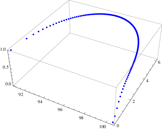
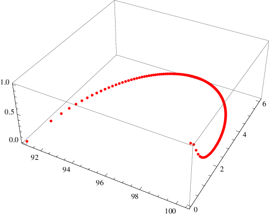
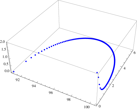
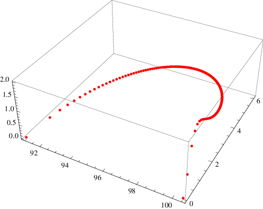
A numerical plot of the functions is given in Figure 4 and 5. The six dimensional moduli space is a deformation of , preserving an isometry.
The first order terms in the D0-brane action are
| (104) |
which describe the motion of the particle in the presence of units of magnetic flux through and .
We may add a total derivative term to the action and put it in a form where the physical interpretation becomes manifest,
| (105) |
Now, it is interesting to look at this action at the point in the plane that naturally corresponds to the moduli space of vortex solitons that we have found at weak coupling. This is the point or equivalently . At this point where vanishes, the action is precisely that of a particle moving on with radius , in the presence of a Dirac monopole connection of strength ,
| (106) |
Note that this is the Dirac monopole connection on the “north pole” patch, and is singular at the south pole. This is similar to the non-Abelian Chern-Simons vortex discussed in [16]. At the classical level, it appears consistent to identify this as the moduli space action for the vortex soliton we found at weak coupling since it preserves the same symmetries. It is interesting that the radius of this sphere is quantized and determined by the Chern-Simons level . This also appears to be manifest at weak coupling where the radius of the fuzzy two-sphere in the Higgs vacuum, in Eq.(26), after dividing out by a factor of to normalize the corrdinates, is proportional to .
5 Discussion and Conclusions
In this paper, we found -BPS vortex solitons in the mass deformation of ABJM theory. We verified that they preserve six supercharges. These vortices in the Higgs vacuum have internal, non-Abelian, orientational collective coordinates which are responsible for a moduli space of solutions. We also obtained the strong coupling gravity dual of the mass deformed theory and its Higgs vacuum, by performing a quotient on the solution found in [27, 29]. Probe D0-branes in this background correspond to the Chern-Simons vortices. We found that the probe D0-brane exhibits a much larger moduli space than expected for the classical vortex soliton. Within this larger moduli space we could however identify a section which coincides with the classical moduli space of solutions originating from the breaking of a colour-flavour locked symmetry. The dynamics on this section is that of a point particle moving on a sphere of radius coupled to a Dirac monopole field of strength .
The enlarged moduli space at strong coupling leaves us with a puzzle. We think that the extra four dimensions in the moduli space are an artifact of the strong coupling limit and of the supergravity approximation. Another possible explanation could be that we have not found the most general vortex solution because our ansatz was not sufficiently general. We believe that the latter explanation is unlikely - it appears difficult to arrive at a reasonable ansatz that could realize this possibility. Also, as discussed in Section (3.5), the number of fermionic zero modes (which has been computed for in Appendix A) does not suggest the existence of extra bosonic zero modes. Another particularly interesting feature of our solution, which introduces further subtleties, is that the colour-flavour locked symmetry actually involves a locking between an R-symmetry and the global gauge rotations. This is unusual in that although a static vortex solution preserves six supercharges, an adiabatic variation of the internal orientational modulus preserves only two supercharges. The full implications of this for the vortex effective theory also need to be understood.
Acknowledgements: We would like to thank Tim Hollowood and Dave Tong for discussions.
Appendix A: Fermionic zero modes for
In this appendix we compute the number of fermionic zero modes on the vortex background for . The equations for the two sectors and decouple from each other and can be analyzed separately. We find four real zero modes in each sector.
A.1 sector
On the vortex background, the fermionic part of the action for this sector can be written as:
| (107) |
The following Dirac equations are found:
Let us write explicitly the equations for . The following notation is used:
| (108) |
We get two systems of two coupled equations and four decoupled equations:
| (109) |
| (110) |
| (111) |
| (112) |
| (113) |
| (114) |
It is straightforward to check that Eqs. (111), (112) have no square-integrable solutions. Using the BPS equations, we get the system:
| (115) |
then acting with on the first equation we get , which has no square-integrable solutions. Eqs. (113), (114) also does not give any zero modes, they correspond to a 2-dimensional fermion with a Dirac mass term in the background of a vortex (this case is studied in [52]).
Let us go back to the two systems (109), (110). They are trivially related by a complex conjugation. Let us use the variables and :
| (116) |
After a change of the matrices basis, the equations become:
| (117) |
The problem is reduced to the one of finding the kernel of the operator:
| (118) |
acting on . Let us introduce the ausiliary operators
| (119) |
A computation with the index theorem [46, 53] tell us that
The operators and have a trivial kernel; index theorem then can be used to show that and have a kernel with real dimension two. This shows that
A related calculation can be found in [54]. We get 4 fermionic zero modes from the sector.
A.2 sector
The relevant fermionic action is:
| (120) |
The Dirac equations follow:
Let us again specialize to . The following notation is used:
| (121) |
The details of the calculations are rather similar to the ones for the sector. We get two systems of two coupled equations and four decoupled equations:
| (122) |
| (123) |
| (124) |
| (125) |
| (126) |
| (127) |
The four decoupled equations (124)-(127) have no square-integrable solutions.
The two systems (122) and (123) are equivalent. Let us use the variables and :
| (128) |
Changing the matrices basis:
| (129) |
The problem is reduced to the one of finding the kernel of the following operator:
| (130) |
The following ausiliary operators are introduced:
| (131) |
A computation with the index theorem also tell us that
The operators and have a trivial kernel; index theorem then can be used to show that and have a kernel with real dimension two. We get a total of four zero modes from the sector.
References
- [1] A. Hanany and D. Tong, JHEP 0307, 037 (2003) [arXiv:hep-th/0306150].
- [2] R. Auzzi, S. Bolognesi, J. Evslin, K. Konishi and A. Yung, Nucl. Phys. B 673, 187 (2003) [arXiv:hep-th/0307287].
- [3] M. Shifman and A. Yung, Phys. Rev. D 70 (2004) 045004 [arXiv:hep-th/0403149].
- [4] A. Hanany and D. Tong, JHEP 0404, 066 (2004) [arXiv:hep-th/0403158].
- [5] O. Aharony, O. Bergman, D. L. Jafferis and J. Maldacena, JHEP 0810 (2008) 091 [arXiv:0806.1218 [hep-th]].
- [6] J. Gomis, D. Rodriguez-Gomez, M. Van Raamsdonk and H. Verlinde, JHEP 0809 (2008) 113 [arXiv:0807.1074 [hep-th]].
- [7] H. J. de Vega and F. A. Schaposnik, Phys. Rev. Lett. 56, 2564 (1986); S. K. Paul and A. Khare, Phys. Lett. B 174, 420 (1986) [Erratum-ibid. 177B, 453 (1986)].
- [8] J. Hong, Y. Kim and P. Y. Pac, Phys. Rev. Lett. 64 (1990) 2230.
- [9] R. Jackiw and E. J. Weinberg, Phys. Rev. Lett. 64 (1990) 2234; R. Jackiw, K. M. Lee and E. J. Weinberg, Phys. Rev. D 42 (1990) 3488.
- [10] R. Jackiw and S. Y. Pi, Phys. Rev. D 42, 3500 (1990) [Erratum-ibid. D 48, 3929 (1993)].
- [11] K. M. Lee, Phys. Rev. Lett. 66 (1991) 553; K. M. Lee, Phys. Lett. B 255 (1991) 381.
- [12] C. k. Lee, K. M. Lee and E. J. Weinberg, Phys. Lett. B 243 (1990) 105.
- [13] G. V. Dunne, arXiv:hep-th/9902115.
- [14] P. A. Horvathy and P. Zhang, arXiv:0811.2094 [hep-th].
- [15] L. G. Aldrovandi and F. A. Schaposnik, Phys. Rev. D 76, 045010 (2007) [arXiv:hep-th/0702209]; G. S. Lozano, D. Marques, E. F. Moreno and F. A. Schaposnik, Phys. Lett. B 654, 27 (2007) [arXiv:0704.2224 [hep-th]]; M. Buck, E. F. Moreno and F. A. Schaposnik, J. Phys. A 42, 205401 (2009) [arXiv:0902.0738 [hep-th]].
- [16] B. Collie and D. Tong, Phys. Rev. D 78, 065013 (2008) [arXiv:0805.0602 [hep-th]].
- [17] B. Collie, J. Phys. A 42, 085404 (2009) [arXiv:0809.0394 [hep-th]].
- [18] S. B. Gudnason, arXiv:0906.0021 [hep-th].
- [19] Y. Kim and K. M. Lee, Phys. Rev. D 49, 2041 (1994) [arXiv:hep-th/9211035]; Y. b. Kim and K. M. Lee, Phys. Rev. D 66, 045016 (2002) [arXiv:hep-th/0204111].
- [20] J. Bagger and N. Lambert, Phys. Rev. D 75 (2007) 045020 [arXiv:hep-th/0611108]; J. Bagger and N. Lambert, Phys. Rev. D 77 (2008) 065008 [arXiv:0711.0955 [hep-th]]; J. Bagger and N. Lambert, JHEP 0802 (2008) 105 [arXiv:0712.3738 [hep-th]].
- [21] A. Gustavsson, Nucl. Phys. B 811 (2009) 66 [arXiv:0709.1260 [hep-th]].
- [22] K. Hosomichi, K. M. Lee, S. Lee, S. Lee, J. Park and P. Yi, JHEP 0811, 058 (2008) [arXiv:0809.1771 [hep-th]].
- [23] K. Hosomichi, K. M. Lee and S. Lee, Phys. Rev. D 78 (2008) 066015 [arXiv:0804.2519 [hep-th]].
- [24] J. Kim and B. H. Lee, JHEP 0901 (2009) 001 [arXiv:0810.3091 [hep-th]].
- [25] M. Arai, C. Montonen and S. Sasaki, JHEP 0903 (2009) 119 [arXiv:0812.4437 [hep-th]].
- [26] S. Kawai and S. Sasaki, arXiv:0903.3223 [hep-th].
- [27] I. Bena and N. P. Warner, JHEP 0412, 021 (2004) [arXiv:hep-th/0406145].
- [28] I. Bena, Phys. Rev. D 62, 126006 (2000) [arXiv:hep-th/0004142].
- [29] H. Lin, O. Lunin and J. M. Maldacena, JHEP 0410, 025 (2004) [arXiv:hep-th/0409174].
- [30] K. Hosomichi, K. M. Lee, S. Lee, S. Lee and J. Park, JHEP 0809, 002 (2008) [arXiv:0806.4977 [hep-th]].
- [31] R. C. Myers, JHEP 9912 (1999) 022 [arXiv:hep-th/9910053].
- [32] H. Nastase, C. Papageorgakis and S. Ramgoolam, arXiv:0903.3966 [hep-th].
- [33] R. Donagi and E. Witten, Nucl. Phys. B 460, 299 (1996) [arXiv:hep-th/9510101].
- [34] J. Polchinski and M. J. Strassler, arXiv:hep-th/0003136.
- [35] R. P. Andrews and N. Dorey, Nucl. Phys. B 751 (2006) 304 [arXiv:hep-th/0601098].
- [36] V. Markov, A. Marshakov and A. Yung, Nucl. Phys. B 709 (2005) 267 [arXiv:hep-th/0408235].
- [37] R. Auzzi and S. Prem Kumar, JHEP 0812, 077 (2008) [arXiv:0810.3201 [hep-th]].
- [38] C. Kim, Y. Kim, O. K. Kwon and H. Nakajima, arXiv:0905.1759 [hep-th].
- [39] M. Benna, I. Klebanov, T. Klose and M. Smedback, JHEP 0809, 072 (2008) [arXiv:0806.1519 [hep-th]].
- [40] W. Nahm, Nucl. Phys. B 135 (1978) 149.
- [41] H. Lin and J. M. Maldacena, Phys. Rev. D 74 (2006) 084014 [arXiv:hep-th/0509235].
- [42] A. Abrikosov, Sov. Phys. JETP 32, 1442 (1957); H. Nielsen and P. Olesen, Nucl. Phys. B61, 45 (1973).
- [43] V. Borokhov, A. Kapustin and X. k. Wu, JHEP 0211 (2002) 049 [arXiv:hep-th/0206054]; V. Borokhov, A. Kapustin and X. k. Wu, JHEP 0212 (2002) 044 [arXiv:hep-th/0207074].
- [44] M. Van Raamsdonk, JHEP 0805 (2008) 105 [arXiv:0803.3803 [hep-th]].
- [45] S. Terashima, JHEP 0808 (2008) 080 [arXiv:0807.0197 [hep-th]].
- [46] E. J. Weinberg, Phys. Rev. D 19 (1979) 3008.
- [47] T. T. Wu and C. N. Yang, Nucl. Phys. B 107 (1976) 365.
- [48] E. D’Hoker and L. Vinet, Phys. Lett. B 137 (1984) 72; F. De Jonghe, A. J. Macfarlane, K. Peeters and J. W. van Holten, Phys. Lett. B 359 (1995) 114 [arXiv:hep-th/9507046].
- [49] S. T. Hong, J. Lee, T. H. Lee and P. Oh, Phys. Lett. B 628 (2005) 165 [arXiv:hep-th/0507194]; S. T. Hong, J. Lee, T. H. Lee and P. Oh, JHEP 0602 (2006) 036 [arXiv:hep-th/0511275]; S. T. Hong, J. Lee, T. H. Lee and P. Oh, Mod. Phys. Lett. A 22 (2007) 1481 [arXiv:hep-th/0606202].
- [50] A. Agarwal, N. Beisert and T. McLoughlin, JHEP 0906 (2009) 045 [arXiv:0812.3367 [hep-th]].
- [51] E. A. Bergshoeff and O. Hohm, Phys. Rev. D 78 (2008) 125017 [arXiv:0810.0377 [hep-th]].
- [52] H. J. de Vega, Phys. Rev. D 18 (1978) 2932.
- [53] E. J. Weinberg, Phys. Rev. D 24 (1981) 2669.
- [54] B. H. Lee, C. k. Lee and H. Min, Phys. Rev. D 45 (1992) 4588.