Variational characterisation of Gibbs measures with Delaunay triangle interaction

David Dereudre¹¹ 1 LAMAV, Université de Valenciennes et du Hainaut-Cambrésis, Le Mont Houy 59313 Valenciennes Cedex 09, France. E-mail: david.dereudre@univ-valenciennes.fr Hans-Otto Georgii²² 2 Mathematisches Institut der Universität München, Theresienstraße 39, 80333 München, Germany. E-mail: georgii@math.lmu.de

August 9, 2026

Abstract

This paper deals with stationary Gibbsian point processes on the plane with an interaction that depends on the tiles of the Delaunay triangulation of points via a bounded triangle potential. It is shown that the class of these Gibbs processes includes all minimisers of the associated free energy density and is therefore nonempty. Conversely, each such Gibbs process minimises the free energy density, provided the potential satisfies a weak long-range assumption.

Keywords. Delaunay triangulation, Voronoi tessellation, Gibbs measure, variational principle, free energy, pressure, large deviations.
MSC. Primary 60K35; Secondary: 60D05, 60G55, 82B21.
Running head. Delaunay-Gibbs measures

1 Introduction

It is well-known that stationary renewal processes with a reasonable spacing distribution can be characterised as Gibbs processes for an interaction between nearest-neighbour pairs of points [16, Section 6]. Here we consider an analogue in two dimensions, viz. Gibbsian point processes on $\mathbb{R}^{2}$ with an interaction depending on nearest-neighbour triples of points, where the nearest-neighbour triples are defined in terms of the Delaunay triangulation. Recall that the Delaunay triangulation is dual to the Voronoi tessellation, in the sense that two points are connected by a Delaunay edge if and only if their Voronoi cells have a common edge. Since the Voronoi cell of a point consists of the part of space that is closer to this point than to any other point, this means that the Delaunay graph defines a natural nearest-neighbour structure between the points. (Of course, the analogy with renewal processes does not reach too far because the independence of spacings under the Palm distribution, which is characteristic of one-dimensional renewal processes, is lost in two dimensions due to the geometric constraints.)

There is a principal difference between the Delaunay interactions considered here and the pair interactions that are common in Statistical Physics. Namely, suppose a point configuration $\omega$ is augmented by a new particle at $x$ . In the case of pair interactions, $x$ is subject to some additional interaction with the particles in $\omega$ , but the interaction between the particles of $\omega$ is not affected by $x$ . In the Delaunay case, however, the particle at $x$ not only gives rise to some new tiles of the Delaunay triangulation, but also destroys some other tiles that were present in the triangulation of $\omega$ . This so-called non-hereditary nature of the Delaunay triangulation blurs the usual distinction between attractive and repulsive interactions and makes it difficult to use a local characterisation of Gibbs measures in terms of their Campbell measures and Papangelou intensities. Such a local approach to the existence of Gibbs measures for Delaunay interactions was used in the previous work [2, 3, 5, 7] and made it necessary to impose geometric constraints on the interaction by removing triangles with small angles or large circumcircles.

In this paper we address the existence problem from a global point of view, which is based on stationarity and thermodynamic quantities such as pressure and free energy density. Specifically, we show that all minimisers of the free energy density are Gibbsian, which implies the existence of Delaunay-Gibbs measures because the entropy density has compact level sets. The converse part of this variational principle is harder and requires the comparison of different boundary conditions in the thermodynamic limit. It is here that the non-hereditary nature of the interaction shows up again, but it can be controlled with the help of stationarity and an additional condition which is much weaker than the geometric constraints mentioned above. In contrast to [7], however, we need to assume throughout that the interaction potential is bounded, and therefore do not cover hard-core interactions that forbid particular shapes of the tiles. We note, however, that some ideas of the present paper can be used to establish the existence of Delaunay-Gibbs measures in a more general setting that includes also the hard-core case, see [8]. The extension of the variational principle to such interactions is left to future work. As a final comment, let us emphasise that we make repeated use of Euler’s polyhedral formula and the resulting linear complexity of the Delaunay triangulations, and are therefore limited to two dimensions, as was already the case in the previous papers mentioned above.

2 Preliminaries

2.1 Configurations and Delaunay triangulations

A subset $\omega$ of $\mathbb{R}^{2}$ is called locally finite if $\text{\rm card\hskip 1.0pt}(\omega\cap\Delta)<\infty$ for all bounded $\Delta\subset\mathbb{R}^{2}$ ; each such $\omega$ is called a configuration. We write $\Omega$ for the set of all configurations $\omega$ . The configuration space $\Omega$ is equipped with the $\sigma$ -algebra $\mathcal{F}$ that is generated by the counting variables $N_{\Delta}:\omega\to\text{\rm card\hskip 1.0pt}(\omega\cap\Delta)$ , with $\Delta$ an arbitrary bounded Borel subset of $\mathbb{R}^{2}$ .

For each Borel set $\Lambda\subset\mathbb{R}^{2}$ we write $\Omega_{\Lambda}=\{\omega\in\Omega:\omega\subset\Lambda\}$ for the set of configurations in $\Lambda$ , $\text{\rm pr}_{\Lambda}:\omega\to\omega_{\Lambda}:=\omega\cap\Lambda$ for the projection from $\Omega$ to $\Omega_{\Lambda}$ , $\mathcal{F}_{\Lambda}^{\prime}=\mathcal{F}|\Omega_{\Lambda}$ for the trace $\sigma$ -algebra of $\mathcal{F}$ on $\Omega_{\Lambda}$ , and $\mathcal{F}_{\Lambda}=\text{\rm pr}_{\Lambda}^{-1}\mathcal{F}_{\Lambda}^{\prime}$ for the $\sigma$ -algebra of events in $\Omega$ that happen in $\Lambda$ only.

For each configuration $\omega\in\Omega$ we consider the Delaunay triangulation $\mathsf{D}(\omega)$ associated to $\omega$ . By definition,

(2.1)

\mathsf{D}(\omega)=\big\{\tau\subset\omega:\ \text{\rm card\hskip 1.0pt}\tau=3,\,\omega\cap B(\tau)=\emptyset\big\}\,,

where $B(\tau)$ is the unique open disc with $\tau\subset\partial B(\tau)$ . $\mathsf{D}(\omega)$ is uniquely defined and determines a triangulation of the convex hull of $\omega$ whenever $\omega$ is in general circular position, in that no four points of $\omega$ lie on a circle that contains no further points of $\omega$ inside [17]. If this is not the case, one can apply some determistic rule to make the Delaunay triangulation unique. Indeed, let

\mathcal{T}:=\big\{\tau\subset\mathbb{R}^{2}:\;\text{\rm card\hskip 1.0pt}\tau=3\big\}=\big\{(x,y,z)\in(\mathbb{R}^{2})^{3}:x\prec y\prec z\big\}

be the set of all triangles (or tiles) in $\mathbb{R}^{2}$ where ‘ $\prec$ ’ stands for the lexicographic order in $\mathbb{R}^{2}$ . The triangles in $\mathcal{T}$ can be compared by the lexicographic order of $(\mathbb{R}^{2})^{3}$ , and this in turn induces a lexicographic order on finite collections of triangles. Now, if $n\geq 4$ points of $\omega$ lie on a circle with no points inside then the associated Delaunay cell is a convex polygon having these $n$ points as vertices. To define a unique triangulation of this polygon one can then simply take the smallest among all possible triangulations. Conflicts with other possible polygons cannot arise because the tessellations inside and outside a fixed convex polygon do not depend on each other.

Let us note that the prescription $\omega\to\mathsf{D}(\omega)$ is a mapping from $\Omega$ to the set $\Omega(\mathcal{T})$ of all locally finite subsets of $\mathcal{T}$ . If $\Omega(\mathcal{T})$ is equipped with the $\sigma$ -algebra $\mathcal{F}(\mathcal{T})$ that is defined in analogy to $\mathcal{F}$ , one can easily check that this mapping is measurable.

Next we assign to each tile $\tau\in\mathcal{T}$ a centre and a radius. Specifically, for every $\tau\in\mathcal{T}$ we write $c(\tau)$ for the centre and $\varrho(\tau)$ for the radius of the circumscribed disc $B(\tau)$ . The centres allow us to consider $\mathsf{D}(\omega)$ as a germ-grain system, i.e., as a marked point configuration of germs in $\mathbb{R}^{2}$ and marks in the space

\mathcal{T}_{0}=\{\tau\in\mathcal{T}:\;c(\tau)=0\}

of centred tiles, by considering the mapping

(2.2)

D:\omega\to\big\{(c(\tau),\tau-c(\tau)):\tau\in\mathsf{D}(\omega)\big\}

from $\Omega$ to the point configurations on $\mathbb{R}^{2}\times\mathcal{T}_{0}$ . Here we write $\tau-c(\tau):=\{y-c(\tau):y\in\tau\}$ for the shifted tile.

A crucial fact we need in the following is the linear complexity of Delaunay triangulations, which is expressed in the following lemma. This result follows directly from Euler’s polyhedral formula, and is the main reason why we need to confine ourselves to two spatial dimensions; see [1], Chapter 11, and [17], Remark 2.1.4.

Lemma 2.1

For a simple planar graph on $n$ vertices, the number of edges is at most $3n-6$ , and the number of inner faces is at most $2n-5$ . In particular, every triangulation with $n$ nodes consists of $2n-2-\partial$ triangles, where $\partial$ is the number of nodes (or: number of edges) along the outer boundary.

2.2 Stationary point processes and their tile distribution

Let $\mathscr{P}_{\Theta}$ be the set of all probability measures $P$ on $(\Omega,\mathcal{F})$ that satisfy the following two properties:

(S)

$P$ is stationary, that is, $P$ is invariant under the shift group $\Theta=(\vartheta_{x})_{x\in\mathbb{R}^{2}}$ on $\Omega$ , which is defined by $\vartheta_{x}:\omega\to\omega-x:=\{y-x:y\in\omega\}$ .
(I)

$P$ has a finite intensity $z(P)=|\Delta|^{-1}\int N_{\Delta}\,dP<\infty$ . Here, $\Delta$ is any bounded Borel set in $\mathbb{R}^{2}$ (which can be arbitrarily chosen due to stationarity), and $|\Delta|$ its Lebesgue measure.

Each $P\in\mathscr{P}_{\Theta}$ is called a stationary point process on $\mathbb{R}^{2}$ with finite intensity. For $\Lambda\subset\mathbb{R}^{2}$ , we write $P_{\Lambda}:=P\circ\text{\rm pr}_{\Lambda}^{-1}$ for the projection image of $P$ on $(\Omega_{\Lambda},\mathcal{F}_{\Lambda}^{\prime})$ , which can of course be identified with the restriction $P|\mathcal{F}_{\Lambda}$ of $P$ to the events in $\Lambda$ .

Every $P\in\mathscr{P}_{\Theta}$ defines a germ-grain model $\bar{P}$ , namely the distribution of $P$ under the mapping $D$ defined in (2.2). That is, $\bar{P}$ is a stationary marked point process on $\mathbb{R}^{2}$ with mark space $\mathcal{T}_{0}$ . Let $\bar{P}^{0}$ be the associated Palm measure on $\mathcal{T}_{0}\times\Omega$ and $\mu_{P}=\bar{P}^{0}(\,\cdot\,\times\Omega)$ the associated mark distribution, or centred tile distribution, on $\mathcal{T}_{0}$ . By definition,

(2.3)

\int dx\int\mu_{P}(d\tau)\,f(x,\tau)=\int P(d\omega)\sum_{\tau\in\mathsf{D}(\omega)}f(c(\tau),\tau-c(\tau))

for all nonnegative measurable functions $f$ on $\mathbb{R}^{2}\times\mathcal{T}_{0}$ . For each $P\in\mathscr{P}_{\Theta}$ , $\mu_{P}$ has total mass $\|\mu_{P}\|=2z(P)$ , as follows from Euler’s polyhedral formula; see, for example, [17, Eq. (3.2.11)] or [20, Theorem 10.6.1(b)].

Let us say a measure $P\in\mathscr{P}_{\Theta}$ is tempered if

(2.4)

\int|B(\tau)|\,\mu_{P}(d\tau)<\infty

We write $\mathscr{P}_{\Theta}^{\text{\rm tp}}$ for the set of all tempered $P\in\mathscr{P}_{\Theta}$ . Of course, (2.4) is equivalent to the condition $\int\varrho(\tau)^{2}\,\mu_{P}(d\tau)<\infty$ . Moreover, (2.3) implies that

(2.5)				$\displaystyle\int\|B(\tau)\|\,\mu_{P}(d\tau)=\int dx\int\mu_{P}(d\tau)\,\mathds{1}_{\{x\in B(\tau)\}}$
(2.5)			$\displaystyle=$	$\displaystyle\int\sum_{\tau\in\mathsf{D}(\omega)}\mathds{1}_{\{c(\tau)\in B(\tau-c(\tau))\}}\,P(d\omega)=\int\text{\rm card\hskip 1.0pt}\big\{\tau\in\mathsf{D}(\omega):0\in B(\tau)\big\}\,P(d\omega)\,.$

So, $P$ is tempered if and only if the last expression is finite. A sufficient condition for temperedness will be given in Proposition 4.9.

The most prominent members of $\mathscr{P}_{\Theta}^{\text{\rm tp}}$ are the Poisson point processes, which will take the role of reference processes for the models we consider. Recall that the Poisson point process $\Pi^{z}$ with intensity $z>0$ is characterised by the following two properties:

(P1)

For every bounded Borel set $\Delta$ , the counting variable $N_{\Delta}$ is Poisson distributed with parameter $z|\Delta|$ .
(P2)

Conditional on $N_{\Delta}=n$ , the $n$ points in $\Delta$ are independent with uniform distribution on $\Delta$ , for every bounded Borel set $\Delta$ and each integer $n$ .

The temperedness of $\Pi^{z}$ follows from Proposition 4.3.1 of [17], or Proposition 4.9 below.

Another type of measures in $\mathscr{P}_{\Theta}^{\text{\rm tp}}$ are the stationary empirical fields that are defined as follows. Let $\Lambda\subset\mathbb{R}^{2}$ be an open square of side length $L$ , and for $\omega\in\Omega_{\Lambda}$ let $\omega_{\Lambda,\text{\rm per}}=\{x+Li:\,x\in\omega,\,i\in\mathbb{Z}^{2}\}$ be its periodic continuation. The associated stationary empirical field is then given by

(2.6)

R_{\Lambda,\omega}=\frac{1}{|\Lambda|}\int_{\Lambda}\delta_{\vartheta_{x}\omega_{\Lambda,\text{\rm per}}}\;dx\,.

It is clear that $R_{\Lambda,\omega}$ is stationary. In addition, it is tempered because $2\varrho(\tau)\leq\text{diam\,}\Lambda$ for each triangle $\tau\in\mathsf{D}(\omega_{\Lambda,\text{\rm per}})$ .

2.3 The topology of local convergence

In contrast to the traditional weak topology on the set $\mathscr{P}_{\Theta}$ of stationary point processes, we exploit here a finer topology, which is such that the intensity is a continuous function, but nonetheless the entropy density has compact level sets.

Let $\mathcal{L}$ denote the class of all measurable functions $f:\Omega\to\mathbb{R}$ which are local and tame, in that there exists some bounded Borel set $\Delta\subset\mathbb{R}^{2}$ such that $f=f\circ\text{\rm pr}_{\Delta}$ and $|f|\leq b(1+N_{\Delta})$ for some constant $b=b(f)<\infty$ . The topology $\mathscr{T}_{\mathcal{L}}$ of local convergence on $\mathscr{P}_{\Theta}$ is then defined as the weak* topology induced by $\mathcal{L}$ , i.e., as the smallest topology for which the mappings $P\to\int f\,dP$ with $f\in\mathcal{L}$ are continuous. By the definition of the intensity, it is then clear that the mapping $P\to z(P)$ is continuous.

A further basic continuity property is the fact that the centred tile distribution $\mu_{P}$ depends continuously on $P$ . Let $\mathcal{L}_{0}$ be the class of all bounded measurable functions on the space $\mathcal{T}_{0}$ of centred tiles, and $\mathscr{T}_{0}$ the associated weak* topology on the set $\mathcal{M}(\mathcal{T}_{0})$ of all finite measures on $\mathcal{T}_{0}$ . (This is sometimes called the $\tau$ -topology.)

Proposition 2.2

Relative to the topologies $\mathscr{T}_{\mathcal{L}}$ and $\mathscr{T}_{0}$ introduced above, the mapping $P\to\mu_{P}$ from $\mathscr{P}_{\Theta}$ to $\mathcal{M}(\mathcal{T}_{0})$ is continuous.

This result will be proved in Section 4.1. It takes advantage of the linear complexity of finite Delaunay triangulations, and therefore relies on the planarity of our model.

2.4 The entropy density

Given a point process $P\in\mathscr{P}_{\Theta}$ and a bounded Borel set $\Lambda$ in $\mathbb{R}^{2}$ , we let $I_{\Lambda}(P,\Pi^{z})$ denote the relative entropy (or Kullback-Leibler information) of $P_{\Lambda}$ relative to $\Pi^{z}_{\Lambda}$ . By the independence properties of $\Pi^{z}$ , these quantities are subadditive in $\Lambda$ , which implies that the limit

(2.7)

I_{z}(P)=\lim_{|\Lambda|\to\infty}I_{\Lambda}(P;\Pi^{z})/|\Lambda|\in[0,\infty]

exists and is equal to the supremum of this sequence. For our purposes, it is sufficient to take this limit along a fixed sequence of squares; for example, one can take squares with vertex coordinates in $\mathbb{Z}+1/2$ . The claim then follows from the well-known analogous result for lattice models [10, Chapter 15] by dividing $\mathbb{R}^{2}$ into unit squares. $I_{z}$ is called the (negative) entropy density with reference measure $\Pi^{z}$ .

We set $I=I_{1}$ . Each $I_{z}$ differs from $I$ only by a constant and a multiple of the particle density. In fact, an easy computation shows that

(2.8)

I(P)=I_{z}(P)+1-z+z(P)\log z\hskip 20.00003pt\text{for all $z>0$ and $P\in\mathscr{P}_{\Theta}$\,.}

A crucial fact we need later is the following result obtained in Lemma 5.2 of [14].

Lemma 2.3

In the topology $\mathscr{T}_{\mathcal{L}}$ , each $I_{z}$ is lower semicontinuous with compact level sets $\{I_{z}\leq c\}$ , $c>0$ .

2.5 Triangle interactions

This paper is concerned with point processes with a particle interaction which is induced by the associated Delaunay triangulation. We stick here to the simplest kind of interaction, which depends only on the triangles that occur in each configuration. Specifically, let $\varphi:\mathcal{T}_{0}\to\mathbb{R}$ be an arbitrary measurable function. It can be extended to a unique shift-invariant measurable function $\varphi$ on $\mathcal{T}$ via $\varphi(\tau):=\varphi(\tau-c(\tau))$ , $\tau\in\mathcal{T}$ . Such a $\varphi$ will be called a triangle potential. We will assume throughout that $\varphi$ is bounded, in that

(2.9)

|\varphi|\leq c_{\varphi}

for some constant $c_{\varphi}<\infty$ . In Theorem 3.4 we will need the following additional condition to prove the temperedness of Gibbs measures. Let us say that a triangle potential $\varphi$ is eventually increasing if there exist a constant $r_{\varphi}<\infty$ and a measurable nondecreasing function $\psi:[r_{\varphi},\infty\/\mathclose{[}\to\mathbb{R}$ such that $\varphi(\tau)=\psi(\varrho(\tau))$ when $\varrho(\tau)\geq r_{\varphi}$ . This condition is clearly satisfied when $\varphi$ is constant for all triangles $\tau$ with sufficiently large radius $\varrho(\tau)$ .

Example 2.4

Here are some examples of triangle potentials. For each triangle $\tau\in\mathcal{T}$ let $b(\tau)=\frac{1}{3}\sum_{x\in\tau}x$ be the barycentre and $A(\tau)$ the area of $\tau$ . Examples of bounded (and scale invariant) interactions that favour equilateral Delaunay triangles are

\varphi_{1}(\tau)=\beta\,|c(\tau)-b(\tau)|/\varrho(\tau)\hskip 10.00002pt\text{ or }\hskip 10.00002pt\varphi_{2}(\tau)=-\beta\,A(\tau)/\varrho(\tau)^{2}

with $\beta>0$ . Of course, many variants are possible; e.g., one can replace the barycentre by the centre of the inscribed circle. By way of contrast, to penalise regular configurations one can replace the $\varphi_{i}$ ’s by their negative.

The triangle potentials $\varphi_{i}$ above are not eventually increasing. But each triangle potential $\varphi$ can be modified to exhibit this property by setting

\tilde{\varphi}(\tau)=\left\{\begin{array}[]{cl}\varphi(\tau)&\text{ if }\varrho(\tau)<r\,,\\ K&\text{ otherwise}\end{array}\right.

with $r>0$ and $K$ a suitable constant. When $K$ is large, one has the additional effect of favouring small circumcircles.

Remark 2.5

The type of interaction introduced above is the simplest possible that is adapted to the Delaunay structure. In particular, we avoid here any explicit interaction $\psi$ along the Delaunay edges. This has two reasons: First, we might add a term of the form $\frac{1}{2}\sum_{e\subset\tau:\,\text{\rm card\hskip 1.0pt}e=2}\varphi_{\text{edge}}(e)$ to the triangle interaction $\varphi$ . Such a term would take account for an edge interaction $\varphi_{\text{edge}}$ whenever $\mathsf{D}(\omega)$ is a triangulation of the full plane. Secondly, we often need to control the interaction over large distances; the condition of $\varphi$ being eventually increasing is tailored for this purpose. It is then essential to define the range in terms of triangles rather than edges. Namely, if a configuration $\omega$ is augmented by a particle at a large distance from $\omega$ , the circumcircles of all destroyed triangles must be large, but their edges can be arbitrarily short. So, a large-circumcircle assumption on the triangle potential allows to control this effect, but a long-edge asumption on an edge potential would be useless.

3 Results

Let $\varphi$ be a fixed triangle potential. We assume throughout that $\varphi$ is bounded, see (2.9), but do not require in general that $\varphi$ is eventually increasing. For each bounded Borel set $\Lambda\subset\mathbb{R}^{2}$ and each configuration $\omega\in\Omega$ , the associated Hamiltonian in $\Lambda$ with boundary condition $\omega$ is then defined for arbitrary $\zeta\in\Omega$ by

(3.1)

H_{\Lambda,\omega}(\zeta)=\sum_{\tau\in\mathsf{D}(\zeta_{\Lambda}\cup\omega_{\Lambda^{c}}):\,B(\tau)\cap\Lambda\neq\emptyset}\varphi(\tau)\,.

It is always well-defined since the sum is finite. Note that $H_{\Lambda,\omega}(\emptyset)\neq 0$ in general. For defining the associated Gibbs distribution we need to impose a condition on the boundary condition $\omega$ .

Definition. Let us say a configuration $\omega\in\Omega$ is admissible if for every bounded Borel set $\Lambda$ there exists a bounded Borel set $\bar{\Lambda}(\omega)\supset\Lambda$ such that $B(\tau)\subset\bar{\Lambda}(\omega)$ whenever $\zeta\in\Omega$ and $\tau\in\mathsf{D}(\zeta_{\Lambda}\cup\omega_{\Lambda^{c}})$ is such that $B(\tau)\cap\Lambda\neq\emptyset$ . We write $\Omega^{*}$ for the set of all admissible configurations.

In Corollary 4.2 we will show that $P(\Omega^{*})=1$ for all $P\in\mathscr{P}_{\Theta}$ with $P(\{\emptyset\})=0$ . Suppose now that $\omega\in\Omega^{*}$ and $\Lambda$ is any bounded Borel set. Lemma 2.1 then shows that

H_{\Lambda,\omega}\geq-2c_{\varphi}N_{\Lambda}-2c_{\varphi}N_{\bar{\Lambda}(\omega)\setminus\Lambda}(\omega)\,,

where $\bar{\Lambda}(\omega)$ is as above. This in turn implies that for each $z>0$ the associated partition function

(3.2)

Z_{\Lambda,z,\omega}=\int e^{-H_{\Lambda,\omega}}\,d\Pi^{z}_{\Lambda}

is finite. We can therefore define the Gibbs distribution with activity $z>0$ by

(3.3)

G_{\Lambda,z,\omega}(A)=Z_{\Lambda,z,\omega}^{-1}\int\mathds{1}_{A}(\zeta\cup\omega_{\Lambda^{c}})\,e^{-H_{\Lambda,\omega}(\zeta)}\,\Pi^{z}_{\Lambda}(d\zeta)\;,\hskip 10.00002ptA\in\mathcal{F}.

The measure $G_{\Lambda,z,\omega}$ depends measurably on $\omega$ and thus defines a probability kernel from $(\Omega^{*},\mathcal{F}_{\Lambda^{c}})$ to $(\Omega,\mathcal{F})$ .

Definition. A probability measure $P$ on $(\Omega,\mathcal{F})$ is called a Gibbs point process for the Delaunay triangle potential $\varphi$ and the activity $z>0$ , or a Delaunay-Gibbs measure for short, if $P(\Omega^{*})=1$ and $P=\int P(d\omega)\,G_{\Lambda,z,\omega}$ for all bounded Borel sets $\Lambda\subset\mathbb{R}^{2}$ . We write $\mathscr{G}_{\Theta}(z,\varphi)$ for the set of all stationary Gibbs measures for $\varphi$ and $z$ , and $\mathscr{G}_{\Theta}^{\text{\rm tp}}(z,\varphi)$ for the set of all tempered stationary Gibbs measures; recall Eq. (2.4).

The above definition corresponds to the classical concept of a Gibbs measure, which is based on the location of points. We note that an alternative concept of Gibbs measure that considers the location of Delaunay triangles has been proposed and used by Zessin [21] and Dereudre [7].

Intuitively, the interaction of a configuration in $\Lambda$ with its boundary condition $\omega$ reaches not farther than the set $\bar{\Lambda}(\omega)$ above, which guarantees some kind of quasilocality. So one can expect that a limit of suitable Gibbs distributions $G_{\Lambda,z,\omega}$ as $\Lambda\uparrow\mathbb{R}^{2}$ should be Gibbsian, and the existence problem reduces to the question of whether such limits exist. Our approach here is to take the necessary compactness property from Lemma 2.3, the compactness of level sets of the entropy density. In fact, we even go one step further and show that the stationary Gibbs measures are the minimisers of the free energy density. Since such minimisers exist by the compactness of level sets, this solves in particular the existence problem. The free energy density is defined as follows; recall the definition of the centred tile distribution $\mu_{P}$ before (2.3).

Definition. The energy density of a stationary point process $P\in\mathscr{P}_{\Theta}$ is defined by

\Phi(P)=\int\varphi\,d\mu_{P}=|\Delta|^{-1}\int P(d\omega)\sum_{\tau\in\mathsf{D}(\omega):\,c(\tau)\in\Delta}\varphi(\tau)\,,

where $\Delta$ is an arbitrary bounded Borel set. The free energy density of $P$ relative to $\Pi^{z}$ is given by $I_{z}(P)+\Phi(P)$ .

The definition of $\Phi$ is justified by Proposition 3.6 below. Here are some crucial facts on the free energy density, which will be proved in Subsection 4.1.

Proposition 3.1

Relative to the topology $\mathscr{T}_{\mathcal{L}}$ on $\mathscr{P}_{\Theta}$ , $\Phi$ is continuous, and each $I_{z}+\Phi$ is lower semicontinuous with compact level sets. In particular, the set $\mathscr{M}_{\Theta}(z,\varphi)$ of all minimisers of $I_{z}+\Phi$ is a non-empty convex compact set, and in fact a face of the simplex $\mathscr{P}_{\Theta}$ .

Next we observe that the elements of $\mathscr{M}_{\Theta}(z,\varphi)$ are nontrivial, in that the empty configuration $\emptyset\in\Omega$ has zero probability; this result will also be proved in Subsection 4.1.

Proposition 3.2

For all $z>0$ we have $\delta_{\emptyset}\notin\mathscr{M}_{\Theta}(z,\varphi)$ , and thus $P(\{\emptyset\})=0$ for all $P\in\mathscr{M}_{\Theta}(z,\varphi)$ .

Our main result is the following variational characterisation of Gibbs measures.

Theorem 3.3

Let $\varphi$ be a bounded triangle potential and let $z>0$ . Then every minimiser of the free energy density is a stationary Gibbs measure. That is, the identity $\mathscr{M}_{\Theta}(z,\varphi)\subset\mathscr{G}_{\Theta}(z,\varphi)$ holds. In particular, Gibbs measures exist. Conversely, every tempered stationary Gibbs measure is a minimiser of the free energy density, which means that $\mathscr{G}^{\text{\rm tp}}_{\Theta}(z,\varphi)\subset\mathscr{M}_{\Theta}(z,\varphi)$ .

The proof will be given in Subsections 4.2 and 4.5. Theorem 3.3 raises the problem of whether all stationary Gibbs measures are tempered. It is natural to expect that $\mathscr{G}_{\Theta}(z,\varphi)=\mathscr{G}^{\text{\rm tp}}_{\Theta}(z,\varphi)$ , but we did not succeed to prove this in general. In fact, we even do not know whether $\mathscr{G}^{\text{\rm tp}}_{\Theta}(z,\varphi)$ is always non-empty. But we can offer the following sufficient condition, which will be proved in Subsection 4.6.

Theorem 3.4

Suppose $\varphi$ is eventually increasing and let $z>0$ . Then every stationary Gibbs measure is tempered, so that $\mathscr{G}^{\text{\rm tp}}_{\Theta}(z,\varphi)=\mathscr{G}_{\Theta}(z,\varphi)$ .

Combining Theorems 3.3 and 3.4 we arrive at the following result.

Corollary 3.5

Suppose $\varphi$ is bounded and eventually increasing, and let $z>0$ . Then the minimisers of the free energy density are precisely the stationary tempered Gibbs measures. That is, $\mathscr{M}_{\Theta}(z,\varphi)=\mathscr{G}_{\Theta}(z,\varphi)=\mathscr{G}_{\Theta}^{\text{\rm tp}}(z,\varphi)$ for all $z>0$ .

The proof of Theorem 3.3 is based on an analysis of the mean energy and the pressure in the infinite volume limit when $\Lambda\uparrow\mathbb{R}^{2}$ . For simplicity, we take this limit through a fixed reference sequence, namely the sequence

(3.4)

\textstyle\Lambda_{n}=\/\big]-n-\frac{1}{2},n+\frac{1}{2}\/\big[^{\;2}

of open centred squares. We shall often write $n$ when we refer to $\Lambda_{n}$ . That is, we set $\omega_{n}=\omega_{\Lambda_{n}}$ , $P_{n}=P_{\Lambda_{n}}$ , $R_{n,\omega}=R_{\Lambda_{n},\omega}$ , $H_{n,\omega}=H_{\Lambda_{n},\omega}$ , and so on. We also write $v_{n}=|\Lambda_{n}|=(2n+1)^{2}$ for the Lebesgue measure of $\Lambda_{n}$ . Our first result justifies the above definition of $\Phi(P)$ . Besides the Hamiltonian (3.1) with configurational boundary condition $\omega$ , we will also consider the Hamiltonian with periodic boundary condition, namely

(3.5)

H_{n,\text{\rm per}}(\omega):=v_{n}\Phi(R_{n,\omega})=\sum_{\tau\in\mathsf{D}(\omega_{n,\text{\rm per}}):\,c(\tau)\in\Lambda_{n}}\varphi(\tau)\;.

By definition, we have $H_{n,\text{\rm per}}(\emptyset)=0$ . Applying Lemma 2.1 and using (2.9), we see that $|H_{n,\text{\rm per}}|\leq v_{n}c_{\varphi}\,2\,z(R_{n})=2c_{\varphi}\,N_{n}$ . The following result will be proved in Subsection 4.1.

Proposition 3.6

For every $P\in\mathscr{P}_{\Theta}$ we have

\lim_{n\to\infty}v_{n}^{-1}\int H_{n,\text{\rm per}}\,dP=\Phi(P)\,.

Moreover, if $P$ is tempered then

\lim_{n\to\infty}v_{n}^{-1}\int H_{n,\omega}(\omega)\,P(d\omega)=\Phi(P)\,.

Finally we turn to the pressure. Let

Z_{n,z,\text{\rm per}}=\int e^{-H_{n,\text{\rm per}}}\,d\Pi^{z}_{n}

be the partition function in $\Lambda_{n}$ with periodic boundary condition.

Proposition 3.7

For each $z>0$ , the pressure

p(z,\varphi):=\lim_{n\to\infty}v_{n}^{-1}\log Z_{n,z,\text{\rm per}}

exists and satisfies

(3.6)

p(z,\varphi)=-\min_{P\in\mathscr{P}_{\Theta}}\big[I_{z}(P)+\Phi(P)\big]\,.

Proof: This is a direct consequence of Theorem 3.1 of [14] because $\Phi$ is continuous by Proposition 3.1. $\Diamond$

A counterpart for the partition functions with configurational boundary conditions follows later in Proposition 4.11. Let us conclude with some remarks on extensions and further results.

Remark 3.8

Large deviations. The following large deviation principle is valid. For every measurable $A\subset\mathscr{P}_{\Theta}$ ,

\limsup_{n\to\infty}v_{n}^{-1}\log G_{n,z,\text{\rm per}}(R_{n}\in A)\leq-\inf I_{z,\varphi}(\text{\rm cl\,}A)

and

\liminf_{n\to\infty}v_{n}^{-1}\log G_{n,z,\text{\rm per}}(R_{n}\in A)\geq-\inf I_{z,\varphi}(\text{\rm int\,}A)\,,

where $G_{n,z,\text{\rm per}}=Z_{n,z,\text{\rm per}}^{-1}e^{-H_{n,\text{\rm per}}}\Pi^{z}_{n}$ is the Gibbs distribution in $\Lambda_{n}$ with periodic boundary condition, $I_{z,\varphi}=I_{z}+\Phi+p(z,\varphi)$ is the excess free energy density, and the closure cl and the interior int are taken in the topology $\mathscr{T}_{\mathcal{L}}$ . Since $\varphi$ is bounded so that $\Phi$ is continuous, this is a direct consequence of Theorem 3.1 of [14].

Remark 3.9

Marked particles. Our results can be extended to the case of point particles with marks, that is, with internal degrees of freedom. Let $E$ be any separable metric space, which is equipped with its Borel $\sigma$ -algebra and a reference measure $\nu$ , and $\overline{\Omega}$ the set of all pairs $\bar{\omega}=(\omega,\sigma_{\omega})$ with $\omega\in\Omega$ and $\sigma_{\omega}\in E^{\omega}$ . In place of the reference Poisson point process $\Pi^{z}$ , one takes the Poisson point process $\overline{\Pi}^{z}$ on $\overline{\Omega}$ with intensity measure $z\lambda\otimes\nu$ , where $\lambda$ is Lebesgue measure on $\mathbb{R}^{2}$ . For $\bar{\omega}\in\overline{\Omega}$ let

\mathsf{D}(\bar{\omega})=\big\{\bar{\tau}=(\tau,\sigma_{\tau}):\tau\in\mathsf{D}(\omega),\ \sigma_{\tau}=\sigma_{\omega}\,|_{\/\tau}\big\}\,.

Of course, the centre, radius and circumscribed disc of a marked triangle $\bar{\tau}$ are still defined in terms of the underlying $\tau$ . In the germ-grain representation, $\mathcal{T}_{0}$ is replaced by the set $\overline{\mathcal{T}_{0}}$ of all centred $\bar{\tau}$ . The tile distribution $\mu_{\bar{P}}$ of a stationary point process $\bar{P}$ on $\overline{\Omega}$ is a finite measure on $\overline{\mathcal{T}_{0}}$ and is defined by placing bars in (2.3). A triangle potential is a bounded function $\varphi$ on $\overline{\mathcal{T}_{0}}$ . Such a $\varphi$ is eventually increasing if $\varphi(\bar{\tau})=\psi(\varrho(\tau))$ for some nondecreasing $\psi$ when $\varrho(\tau)$ is large enough. It is then easily seen that all our arguments carry over to this setting without change.

Remark 3.10

Particles with hard core. There is some interest in the case when the particles are required to have at least some distance $r_{0}>0$ . This is expressed by adding to the Hamiltonian (3.1) a hard-core pair interaction term $H_{\Lambda,\omega}^{\text{\rm hc}}(\zeta)$ which is equal to $\infty$ if $|x-y|\leq r_{0}$ for a pair $\{x,y\}\subset\zeta_{\Lambda}\cup\omega_{\Lambda^{c}}$ with $\{x,y\}\cap\Lambda\neq\emptyset$ , and zero otherwise. Equivalently, one can replace the configuration space $\Omega$ by the space

\Omega^{\text{\rm hc}}=\big\{\omega\in\Omega:|x-y|>r_{0}\text{ for any two distinct }x,y\in\omega\big\}

of all hard-core configurations. The free energy functional on $\mathscr{P}_{\Theta}$ then takes the form $F_{z}^{\text{\rm hc}}:=I_{z}+\Phi+\Phi^{\text{\rm hc}}$ , where

\Phi^{\text{\rm hc}}(P)=\infty\ P^{0}\big(\omega:0<|x|\leq r_{0}\text{ for some }x\in\omega\big)=\infty\ P(\Omega\setminus\Omega^{\text{\rm hc}})

for $P\in\mathscr{P}_{\Theta}$ with Palm measure $P^{0}$ ; here we use the convention $\infty\,0=0$ . We claim that our results can also be adapted to this setting. In particular, the minimisers of $F_{z}^{\text{\rm hc}}$ are Gibbsian for $z$ and the combined triangle and hard-core pair interaction, and the tempered Gibbs measures for this interaction minimise $F_{z}^{\text{\rm hc}}$ . We will comment on the necessary modifications in Remarks 4.4 and 4.12.

Combining the extensions in the last two remarks we can include the following example of phase transition.

Example 3.11

The Delaunay-Potts hard-core model for particles with $q\geq 2$ colours. In the setup of Remark 3.9 we have $E=\{1,\ldots,q\}$ , and the triangle potential is

\varphi(\bar{\tau})=\left\{\begin{array}[]{cl}\beta&\text{if $\varrho(\tau)\leq r_{1}$ and $\sigma_{\tau}$ is not constant,}\\ 0&\text{otherwise,}\end{array}\right.

where $\beta>0$ is the inverse temperature and $r_{1}>0$ is an arbitrary interaction radius. If one adds a hard-core pair interaction with range $r_{0}<r_{1}/\sqrt{2}$ as in Remark 3.10, this model is similar to the model considered in [4]. (Instead of a triangle potential, these authors consider an edge potential along the Delaunay edges that do not belong to a tile $\tau$ of radius $\varrho(\tau)>r_{1}$ .) Using a random cluster representation of the triangle interaction as in [15] and replacing edge percolation by tile percolation one finds that the methods of [4] can be adapted to the present model. Consequently, if $z$ and $\beta$ are sufficiently large, then the simplex $\mathscr{M}_{\Theta}(z,\varphi)=\mathscr{G}_{\Theta}(z,\varphi)$ has at least $q$ distinct extreme points.

4 Proofs

4.1 Energy and free energy

We begin with the proof of Proposition 2.2, which states that the centred tile distribution $\mu_{P}$ depends continuously on $P$ . The continuity of the energy density $\Phi$ and the lower semicontinuity of the free energy density $I_{z}+\Phi$ then follow immediately.

Proof of Proposition 2.2: Let $(P_{\alpha})$ be a net in $\mathscr{P}_{\Theta}$ that converges to some $P\in\mathscr{P}_{\Theta}$ . We need to show that $\int g\,d\mu_{P_{\alpha}}\to\int g\,d\mu_{P}$ for all $g\in\mathcal{L}_{0}$ . We can assume without loss of generality that $0\leq g\leq 1$ .

We first consider the case that $g$ has bounded support, in that $g\leq\mathds{1}\{\varrho\leq r\}$ for some $r>0$ . Let $\Delta\subset\mathbb{R}^{2}$ be any bounded set of Lebesgue measure $|\Delta|=1$ . Also, let

f(\omega)=\sum_{\tau\in\mathsf{D}(\omega)}g(\tau-c(\tau))\,\mathds{1}_{\Delta}(c(\tau))\,.

In view of (2.3), we then have $\int g\,d\mu_{Q}=\int f\,dQ$ for all $Q\in\mathscr{P}_{\Theta}$ , and in particular for $Q=P_{\alpha}$ and $Q=P$ . By the bounded support property of $g$ , $f$ depends only on the configuration in the $r$ -neigbourhood $\Delta^{r}:=\{y\in\mathbb{R}^{2}:|y-x|\leq r\text{ for some }x\in\Delta\}$ of $\Delta$ . That is, $f$ is measurable with respect to $\mathcal{F}_{\Delta^{r}}$ . Moreover, $f\leq 2N_{\Delta^{r}}$ by Lemma 2.1, so that $f\in\mathcal{L}$ . In the present case, the result thus follows from the definition of the topology $\mathscr{T}_{\mathcal{L}}$ .

If $g$ fails to be of bounded support, we can proceed as follows. Let $\varepsilon>0$ be given and $r>0$ be so large that $\mu_{P}(\varrho>r)<\varepsilon$ . Since $\|\mu_{P_{\alpha}}\|=2z(P_{\alpha})\to 2z(P)=\|\mu_{P}\|$ and $\mu_{P_{\alpha}}(\varrho\leq r)\to\mu_{P}(\varrho\leq r)$ by the argument above, we have $\mu_{P_{\alpha}}(\varrho>r)\to\penalty\mu_{P}(\varrho>r)$ . We can therefore assume without loss of generality that $\mu_{P_{\alpha}}(\varrho>r)<\varepsilon$ for all $\alpha$ . Using again the first part of this proof, we can thus write

\begin{split}&\int g\,d\mu_{P}-\varepsilon\leq\int g\,\mathds{1}_{\{\varrho\leq r\}}\,d\mu_{P}=\lim_{\alpha}\int g\,\mathds{1}_{\{\varrho\leq r\}}\,d\mu_{P_{\alpha}}\\ &\leq\liminf_{\alpha}\int g\,d\mu_{P_{\alpha}}\leq\limsup_{\alpha}\int g\,d\mu_{P_{\alpha}}\\ &\leq\lim_{\alpha}\int g\,\mathds{1}_{\{\varrho\leq r\}}\,d\mu_{P_{\alpha}}+\varepsilon=\int g\,\mathds{1}_{\{\varrho\leq r\}}\,d\mu_{P}+\varepsilon\leq\int g\,d\mu_{P}+\varepsilon\,.\end{split}

Since $\varepsilon$ was chosen arbitrarily, the result follows. $\Diamond$

We now turn to the properties of the free energy density.

Proof of Proposition 3.1: As $\varphi$ belongs to $\mathcal{L}_{0}$ , the continuity of $\Phi$ follows immediately from Proposition 2.2. By Lemma 2.3, we can also conclude that $I_{z}+\Phi$ is lower semicontiuous. Moreover, hypothesis (2.9) implies that the level set $\{I_{z}+\Phi\leq c\}$ is contained in $\{I_{z}\leq c+2c_{\varphi}z(\cdot)\}$ , which by (2.8) coincides with the compact set $\{I_{z^{\prime}}\leq c+z^{\prime}-1\}$ for $z^{\prime}=z\exp(2c_{\varphi})$ .

Let $P=\delta_{\emptyset}\in\mathscr{P}_{\Theta}$ be the Dirac measure at the empty configuration. Then $\mu_{P}\equiv 0$ and thus $\Phi(P)=0$ . On the other hand, $I_{z}(P)=z$ . This means that $I_{z}+\Phi$ is not identically equal to $+\infty$ on $\mathscr{P}_{\Theta}$ and thus, by the compactness of its level sets, attains its infimum. To see that the minimisers form a face of $\mathscr{P}_{\Theta}$ , it is sufficient to note that $I_{z}+\Phi$ is measure affine; cf. Theorem (15.20) of [10]. $\Diamond$

Next we show that the minimisers of the free energy are nondegenerate.

Proof of Proposition 3.2: The second statement follows from the first because $\mathcal{M}_{\Theta}(z,\varphi)$ is a face of $\mathscr{P}_{\Theta}$ . For, suppose there exists some $P\in\mathcal{M}_{\Theta}(z,\varphi)$ with $P(\{\emptyset\})>0$ . Then $\delta_{\emptyset}$ appears in the ergodic decomposition of $P$ , which would only be possible if $\delta_{\emptyset}\in\mathcal{M}_{\Theta}(z,\varphi)$ .

To prove the first statement we note that $\Phi(\Pi^{u})\leq c_{\varphi}\|\mu_{\Pi^{u}}\|=2c_{\varphi}u$ for all $u>0$ . Therefore, if $z>0$ is given and $u$ is small enough then

(4.1)

I_{z}(\Pi^{u})+\Phi(\Pi^{u})\leq z-u+u\log(u/z)+2c_{\varphi}u<z=I_{z}(\delta_{\emptyset})+\Phi(\delta_{\emptyset})\,,

so that $\delta_{\emptyset}$ is no minimiser of the free energy. $\Diamond$

Finally we show that the energy density $\Phi$ is the infinite volume limit of the mean energy per volume.

Proof of Proposition 3.6: We begin with the case of periodic boundary conditions. For every $P\in\mathscr{P}_{\Theta}$ , we have $v_{n}^{-1}\int H_{n,\text{\rm per}}\,dP=\int\Phi(R_{n})\,dP=\Phi(PR_{n})$ . It is easy to see that $PR_{n}\to P$ , cf. Remark 2.4 of [14]. Since $\Phi$ is continuous, it follows that $\Phi(PR_{n})\to\Phi(P)$ .

Next we consider the case of configurational boundary conditions and suppose that $P$ is tempered. Applying (2.3) we obtain for each $n$

(4.2)	$\displaystyle\int P(d\omega)\,H_{n,\omega}(\omega)$	$\displaystyle=$	$\displaystyle\int P(d\omega)\sum_{\tau\in\mathsf{D}(\omega)}\varphi(\tau-c(\tau))\,\mathds{1}_{\{B(\tau-c(\tau))\cap(\Lambda_{n}-c(\tau))\neq\emptyset\}}$
		$\displaystyle=$	$\displaystyle\int\mu_{P}(d\tau)\ \varphi(\tau)\int dx\ \mathds{1}_{\{B(\tau)\cap(\Lambda_{n}-x)\neq\emptyset\}}$
		$\displaystyle=$	$\displaystyle\int\mu_{P}(d\tau)\ \varphi(\tau)\,\big\|\Lambda_{n}^{\varrho(\tau)}\big\|,$

where $\Lambda_{n}^{\varrho(\tau)}$ is the $\varrho(\tau)$ -neigbourhood of $\Lambda_{n}$ . Now, for each $\tau$ we have

\big|\Lambda_{n}^{\varrho(\tau)}\big|/v_{n}=1+4\varrho(\tau)/\sqrt{v_{n}}+\pi\varrho(\tau)^{2}/v_{n}\to 1\text{ as }n\to\infty.

In view of (2.4) and (2.9), we can apply the dominated convergence theorem to conclude that

\Phi(P)=\lim_{n\to\infty}v_{n}^{-1}\int H_{n,\omega}(\omega)\,P(d\omega),

as desired. $\Diamond$

4.2 The variational principle: first part

In this section we shall prove that each minimiser of the free energy is a Delaunay-Gibbs measure. We start with an auxiliary result on the ‘range of influence’ of the boundary condition on the events within a bounded set. Let $\Delta\subset\mathbb{R}^{2}$ be a bounded Borel set and $\omega\in\Omega$ . Writing $B(x,r)$ for the open disc in $\mathbb{R}^{2}$ with center $x$ and radius $r$ , we define

\mathcal{R}_{\Delta}(\omega)=\big\{r>0:\ \text{\rm card\hskip 1.0pt}\,\omega_{B(x,r)\setminus\Delta}\geq 1\text{ for all }x\in\mathbb{R}^{2}\text{ s.t. }B(x,r)\cap\Delta\neq\emptyset\big\}

and $\mathbf{r}_{\Delta}(\omega)=\inf\mathcal{R}_{\Delta}(\omega)$ , where $\inf\emptyset:=\infty$ . Let $\Delta^{2r}=\bigcup_{x\in\Delta}B(x,2r)$ be the open $2r$ -neigbourhood of $\Delta$ . We then observe the following.

Lemma 4.1

(a) For all $r>0$ , $\{\mathbf{r}_{\Delta}<r\}\in\mathcal{F}_{\Delta^{2r}\setminus\Delta}$ . In particular, $\mathbf{r}_{\Delta}$ is $\mathcal{F}_{\Delta^{c}}$ -measurable.

(b) For all $P\in\mathscr{P}_{\Theta}$ we have $P(\mathbf{r}_{\Delta}=\infty)=P(\{\emptyset\})$ .

Proof: (a) Let $\tilde{\mathcal{R}}_{\Delta}(\omega)$ be defined as $\mathcal{R}_{\Delta}(\omega)$ , except that the discs are required to have rational centres $x\in\mathbb{Q}^{2}$ . Then $\mathcal{R}_{\Delta}(\omega)\subset\tilde{\mathcal{R}}_{\Delta}(\omega)$ . Moreover, if $r<r^{\prime}$ then every open $r^{\prime}$ -disc intersecting $\Delta$ contains an $r$ -disc with rational center and intersecting $\Delta$ , so that $r^{\prime}\in\mathcal{R}_{\Delta}(\omega)$ when $r\in\tilde{\mathcal{R}}_{\Delta}(\omega)$ . This shows that

\{\mathbf{r}_{\Delta}<r\}=\bigcup_{s\in\mathbb{Q}:\;0<s<r}\ \bigcap_{x\in\mathbb{Q}^{2}:\;B(x,s)\cap\Delta\neq\emptyset}\{N_{B(x,s)\setminus\Delta}\geq 1\}\,,

and the last set certainly belongs to $\mathcal{F}_{\Delta^{2r}\setminus\Delta}$ .

(b) Since $\{\emptyset\}=\bigcap_{r\in\mathbb{N}}\{N_{B(0,r)}=0\}\subset\{\mathbf{r}_{\Delta}=\infty\}$ , it is sufficient to prove that $\{\mathbf{r}_{\Delta}=\infty,N_{B(0,r)}\geq 1\}$ has measure zero for all $r>0$ and $P\in\mathscr{P}_{\Theta}$ . However, if $\{\mathbf{r}_{\Delta}=\infty\}$ occurs then there exists a cone $C$ with apex at some point in the closure of $\Delta$ and an axis in one of finitely many prescribed directions such that $N_{C}=0$ , while the Poincaré recurrence theorem implies that $N_{C}=\infty$ for each such $C$ almost surely on $\{N_{B(0,r)}\geq 1\}$ . This contradiction gives the desired result. $\Diamond$

As an immediate consequence we obtain that each nondegenerate stationary point process is concentrated on the set $\Omega^{*}$ of admissible configurations.

Corollary 4.2

The set $\Omega^{*}$ of admissible configurations is measurable (in fact, shift invariant and tail measurable), and $P(\Omega^{*})=1$ for all $P\in\mathscr{P}_{\Theta}$ with $P(\{\emptyset\})=0$ .

Proof: This is immediate from Lemma 4.1 because $\Omega^{*}=\bigcap_{n\geq 1}\{\mathbf{r}_{\Lambda_{n}}<\infty\}$ . $\Diamond$

Next we state a consequence of Proposition 3.7.

Corollary 4.3

For every $P\in\mathscr{M}_{\Theta}(z,\varphi)$ , we have

\lim_{n\to\infty}v_{n}^{-1}I_{n}(P;G_{n,z,\text{\rm per}})=0\;.

Proof: By the definition of relative entropy,

I_{n}(P;G_{n,z,\text{\rm per}})=I_{n}(P;\Pi^{z})+\int H_{n,\text{\rm per}}\,dP+\log Z_{n,z,\text{\rm per}}\,.

Together with Propositions 3.6 and 3.7, this gives the result. $\Diamond$

We are now ready to show that the minimisers of $I_{z}+\Phi$ are Gibbsian.

Proof of Theorem 3.3, first part: We follow the well-known scheme of Preston [19] (in the variant used in [13], Section 7). Let $P\in\mathscr{M}_{\Theta}(z,\varphi)$ , $f$ be a bounded local function, $\Delta$ a bounded Borel set, and

f_{\Delta}(\omega)=\int f(\zeta)\,G_{\Delta,z,\omega}(d\zeta)\,,\hskip 10.00002pt\omega\in\Omega.

We need to show that $\int f\,dP=\int f_{\Delta}\,dP$ . Let $\mathbf{r}_{\Delta}$ be the range function defined above, and for each $r>0$ let $\mathds{1}_{\Delta,r}=\mathds{1}\{\mathbf{r}_{\Delta}<r\}$ and $\Delta^{2r}$ be the $2r$ -neigbourhood of $\Delta$ . By Lemma 4.1 (a), $\mathds{1}_{\Delta,r}$ is measurable with respect to $\mathcal{F}_{\Delta^{2r}\setminus\Delta}$ . Moreover, if $\mathbf{r}_{\Delta}(\omega)<r$ then $H_{\Delta,\omega}(\zeta)=H_{\Delta,\omega_{\Delta^{2r}\setminus\Delta}}(\zeta)$ for all $\zeta\in\Omega_{\Delta}$ . So, if $r$ is so large that $f$ is $\mathcal{F}_{\Delta^{2r}}$ -measurable, we can conclude that $\mathds{1}_{\Delta,r}\,f_{\Delta}$ is $\mathcal{F}_{\Delta^{2r}\setminus\Delta}$ -measurable.

Now we apply Corollary 4.3, which states that $\lim_{n\to\infty}v_{n}^{-1}I_{\Lambda_{n}}(P;G_{n,z,\text{\rm per}})=0$ . By shift invariance, this implies that $P_{\Lambda}\ll G_{\Lambda,z,\text{\rm per}}$ with a density $g_{\Lambda}$ for each sufficiently large square $\Lambda$ . In particular, for any $\Delta^{\prime}\subset\Lambda$ we have $P_{\Delta^{\prime}}\ll(G_{\Lambda,z,\text{\rm per}})_{\Delta^{\prime}}$ wih density $g_{\Lambda,\Delta^{\prime}}(\omega)=\int G_{\Lambda\setminus\Delta^{\prime},z,\omega\cap\Delta^{\prime}}(d\zeta)\,g_{\Lambda}(\zeta)$ . Corollary 4.3 implies further that for each $\delta>0$ there exists a square $\Lambda$ and a Borel set $\Delta^{\prime}$ with $\Delta^{2r}\subset\Delta^{\prime}\subset\Lambda$ such that $\int|g_{\Lambda,\Delta^{\prime}}-g_{\Lambda,\Delta^{\prime}\setminus\Delta}|\,dG_{\Lambda,z,\text{\rm per}}<\delta$ ; cf. Lemma 7.5 of [13]. Now we consider the difference

\int\mathds{1}_{\Delta,r}\,(f-f_{\Delta})\,dP=\int\mathds{1}_{\Delta,r}\big(g_{\Lambda,\Delta^{\prime}}\,f-g_{\Lambda,\Delta^{\prime}\setminus\Delta}\,f_{\Delta}\big)\,dG_{\Lambda,z,\text{\rm per}}\,.

Since $G_{\Lambda,z,\text{\rm per}}=\int G_{\Lambda,z,\text{\rm per}}(d\omega)\,G_{\Delta,z,\omega}$ and $\mathds{1}_{\Delta,r}\,g_{\Lambda,\Delta^{\prime}\setminus\Delta}$ is $\mathcal{F}_{\Lambda\setminus\Delta}$ -measurable, we can conclude that

\int\mathds{1}_{\Delta,r}\,g_{\Lambda,\Delta^{\prime}\setminus\Delta}\,f_{\Delta}\,dG_{\Lambda,z,\text{\rm per}}=\int\mathds{1}_{\Delta,r}\,g_{\Lambda,\Delta^{\prime}\setminus\Delta}\,f\,dG_{\Lambda,z,\text{\rm per}}\,.

By the choice of $\Lambda$ and $\Delta^{\prime}$ , we can replace the density $g_{\Lambda,\Delta^{\prime}\setminus\Delta}$ in the last expression by $g_{\Lambda,\Delta^{\prime}}$ making an error of at most $\delta$ . We thus find that $\int\mathds{1}_{\Delta,r}\,(f-f_{\Delta})\,dP<\delta$ . Letting $\delta\to 0$ and $r\to\infty$ , we finally obtain by the dominated convergence theorem that

\int_{\{\mathbf{r}_{\Delta}<\infty\}}\,(f-f_{\Delta})\,dP=0\,.

This completes the proof because $P(\mathbf{r}_{\Delta}=\infty)=P(\{\emptyset\})=0$ by Lemma 4.1(b) and Proposition 3.2. $\Diamond$

Remark 4.4

Here are some comments on the necessary modifications in the hard-core setup of Remark 3.10. In analogy to Proposition 3.7, one needs that

\lim_{n\to\infty}v_{n}^{-1}\log\int e^{-H_{n,\text{\rm per}}-H_{n,\text{\rm per}}^{\text{\rm hc}}}\,d\Pi^{z}_{n}=-\min_{P\in\mathscr{P}_{\Theta}}\big[I_{z}(P)+\Phi(P)+\Phi^{\text{\rm hc}}(P)\big]\,.

This follows directly from Propositions 4.1 and 5.4 of [12] because $\Phi$ is continuous. Corollary 4.3 therefore still holds for the periodic Gibbs distributions with additional hard-core pair interaction. One also needs to modify the proof of Proposition 3.2, in that the Poisson processes $\Pi^{u}$ should be replaced by the Gibbs measure $P^{u}$ with activity $u$ and pure hard-core interaction. $P^{u}$ is defined as the limit of the Gibbs distributions $G_{n,u,\text{\rm per}}^{\text{\rm hc}}$ for the periodic hard-core Hamiltonians $H_{n,\text{\rm per}}^{\text{\rm hc}}$ . By Proposition 7.4 of [12], $P^{u}$ exists and satisfies

I_{u}(P^{u})=-\lim_{n\to\infty}v_{n}^{-1}\log\int e^{-H_{n,\text{\rm per}}^{\text{\rm hc}}}\,d\Pi^{u}_{n}\leq-\lim_{n\to\infty}v_{n}^{-1}\log\Pi^{u}_{n}(\{\emptyset\})=u\,.

Together with (2.8) we find that

I_{z}(P^{u})+\Phi(P^{u})\leq z+z(P^{u})\,\big[\log(u/z)+2c_{\varphi}\big]\,,

which is strictly less than $z$ when $u$ is small enough. Since $\Phi^{\text{\rm hc}}(P^{u})=\Phi^{\text{\rm hc}}(\delta_{\emptyset})=0$ , it follows that the minimisers of $I_{z}+\Phi+\Phi^{\text{\rm hc}}$ are non-degenerate. No further changes are required for the proof of the first part of the variational principle.

4.3 Boundary estimates

We now work towards a proof of the reverse part of the variational principle. In this section, we control the boundary effects that determine the difference of $H_{n,\text{\rm per}}$ and $H_{n,\omega}$ . The resulting estimates will be crucial for the proof of Proposition 4.11. For every $\omega\in\Omega$ and every Borel set $\Delta$ let

\mathsf{S}_{\Delta}(\omega)=\big\{\tau\in\mathsf{D}(\omega):B(\tau)\cap\Delta\neq\emptyset\text{ and }B(\tau)\setminus\Delta\neq\emptyset\big\}

be the set of all triangles $\tau\in\mathsf{D}(\omega)$ for which $B(\tau)$ crosses the boundary of $\Delta$ . We start with a lemma that controls the influence on $\mathsf{S}_{\Delta}$ when two configurations are pasted together.

Lemma 4.5

Let $\Delta$ be a (not necessarily bounded) Borel set in $\mathbb{R}^{2}$ , $\zeta\in\Omega^{*}\cup\{\emptyset\}$ a configuraton with $\zeta_{\partial\Delta}=\emptyset$ , and $\omega\in\Omega$ . Then for each $\tau\in\mathsf{S}_{\Delta}(\zeta_{\Delta}\cup\omega_{\Delta^{c}})$ and each $x\in\tau_{\Delta}$ there exists some $\tau^{\prime}\in\mathsf{S}_{\Delta}(\zeta)$ with $x\in\tau^{\prime}$ .

Proof: Let $\Delta$ , $\zeta$ and $\omega$ be given. If $\zeta$ is empty, there exists no $x\in\tau_{\Delta}\subset\zeta_{\Delta}$ , so that the statement is trivially true. So let $\zeta\in\Omega^{*}$ and suppose there exists some $\tau\in\mathsf{S}_{\Delta}(\zeta_{\Delta}\cup\omega_{\Delta^{c}})$ with $\tau_{\Delta}\neq\emptyset$ . Let $x\in\tau_{\Delta}$ . Since $\zeta_{\partial\Delta}=\emptyset$ , $x$ does in fact belong to the interior of $\Delta$ . This implies that $B(\tau^{\prime})\cap\Delta\neq\emptyset$ for each $\tau^{\prime}\in\mathsf{D}(\zeta)$ containing $x$ . Therefore we only need to show that $B(\tau^{\prime})\setminus\Delta\neq\emptyset$ for at least one such $\tau^{\prime}$ . Suppose the contrary. Then $B(\tau^{\prime})\subset\Delta$ whenever $x\in\tau^{\prime}\in\mathsf{D}(\zeta)$ . This means that the Delaunay triangles containing $x$ are completely determined by $\zeta_{\Delta}$ . This gives the contradiction

\emptyset\neq\{\tau\in\mathsf{S}_{\Delta}(\zeta_{\Delta}\cup\omega_{\Delta^{c}}):\tau\ni x\}=\{\tau^{\prime}\in\mathsf{S}_{\Delta}(\zeta):\tau^{\prime}\ni x\}=\emptyset\,,

and the proof is complete. $\Diamond$

The following proposition is the fundamental boundary estimate. It bounds the difference of Hamiltonians with periodic and configurational boundary conditions in terms of $S_{n}:=\text{\rm card\hskip 1.0pt}\mathsf{S}_{\Lambda_{n}}$ .

Proposition 4.6

There exists a universal constant $\gamma<\infty$ such that

|H_{n,\text{\rm per}}(\zeta)-H_{n,\omega}(\zeta)|\leq\gamma c_{\varphi}\,\big(S_{n}(\omega)+S_{n}(\zeta)\big)

for all $n\geq 1$ and all $\zeta,\omega\in\Omega^{*}\cup\{\emptyset\}$ with $\zeta_{\partial\Lambda_{n}}=\omega_{\partial\Lambda_{n}}=\emptyset$ .

Proof: Let $n,\zeta,\omega$ be fixed and

\mathsf{A}=\big\{\tau\in\mathsf{D}(\zeta_{\Lambda_{n}}\cup\omega_{\Lambda_{n}^{c}}):\,B(\tau)\cap\Lambda_{n}\neq\emptyset\big\}\,,\hskip 10.00002pt\mathsf{B}=\big\{\tau\in\mathsf{D}(\zeta_{n,\text{\rm per}}):\,c(\tau)\in\Lambda_{n}\big\}\,.

In view of (3.1) and (3.5) we have $H_{n,\omega}(\zeta)=\sum_{\tau\in\mathsf{A}}\varphi(\tau)$ and $H_{n,\text{\rm per}}(\zeta)=\sum_{\tau\in\mathsf{B}}\varphi(\tau)$ . Since $\varphi$ is bounded by $c_{\varphi}$ , we only need to estimate the cardinalities of $\mathsf{A}\setminus\mathsf{B}$ and $\mathsf{B}\setminus\mathsf{A}$ . We note that $\mathsf{A}\setminus\mathsf{B}\subset\mathsf{S}_{\Lambda_{n}}(\zeta_{\Lambda_{n}}\cup\omega_{\Lambda_{n}^{c}})$ and $\mathsf{B}\setminus\mathsf{A}\subset\mathsf{S}_{\Lambda_{n}}(\zeta_{n,\text{\rm per}})$ . So we can apply Lemma 4.5 to both $\Delta=\Lambda_{n}$ and $\Delta=\Lambda_{n}^{c}$ to obtain that the set of points belonging to a triangle in $\mathsf{A}\setminus\mathsf{B}$ is contained in the set of points belonging to a triangle of $\mathsf{S}_{\Lambda_{n}}(\zeta)\cup\mathsf{S}_{\Lambda_{n}}(\omega)$ . Hence, $\text{\rm card\hskip 1.0pt}\big(\bigcup_{\tau\in\mathsf{A}\setminus\mathsf{B}}\tau\big)\leq 3(S_{n}(\zeta)+S_{n}(\omega))$ . By Lemma 2.1, it follows that $\text{\rm card\hskip 1.0pt}(A\setminus B)\leq 6(S_{n}(\omega)+S_{n}(\zeta))$ .

To estimate the cardinality of $\mathsf{B}\setminus\mathsf{A}$ we may assume that $\zeta_{n}\neq\emptyset$ . The periodic continuation $\zeta_{n,\text{\rm per}}$ then contains a lattice, and this implies that every triangle of $\mathsf{D}(\zeta_{n,\text{\rm per}})$ has a circumscribed disc of diameter at most $\sqrt{2v_{n}}$ . Hence, each $\tau\in\mathsf{B}\setminus\mathsf{A}$ is contained in $\Lambda_{5n+2}$ , the union of $5^{2}$ translates of $\Lambda_{n}$ (up to their boundaries). Applying Lemma 4.5 to each of these translates we conclude that the number of points that belong to a triangle of $\mathsf{B}\setminus\mathsf{A}$ is bounded by $3\cdot 5^{2}\,S_{n}(\zeta)$ . Using Lemma 2.1 again we find that $\text{\rm card\hskip 1.0pt}(B\setminus A)\leq 150(S_{n}(\omega)+S_{n}(\zeta))$ , and the result follows with $\gamma=156$ . $\Diamond$

The following immediate corollary will be needed in the proof of Theorem 3.3.

Corollary 4.7

There exists a constant $C<\infty$ such that $|H_{n,\omega}(\emptyset)|\leq C\,S_{n}(\omega)$ for all $n\geq 1$ and $\omega\in\Omega^{*}$ with $\omega_{\partial\Lambda_{n}}=\emptyset$ .

The next proposition exhibits the fundamental role of the temperedness condition (2.4) combined with stationarity for controlling the boundary effects.

Proposition 4.8

For every $P\in\mathscr{P}_{\Theta}^{\text{\rm tp}}$ , $v_{n}^{-1}S_{n}\to 0$ in $L^{1}(P)$ and $P$ -almost surely.

Proof: For each $i\in\mathbb{R}^{2}$ we consider the shifted unit square $C(i)=\Lambda_{0}+i$ and define the random variable

Z_{i}=\text{\rm card\hskip 1.0pt}\big\{\tau\in\mathsf{D}(\cdot):\,B(\tau)\cap C(i)\neq\emptyset\big\}.

Then

(4.3)

S_{n}\leq\sum_{i\in I_{n}\setminus I_{n-1}}Z_{i}\,,

where $I_{n}=\Lambda_{n}\cap(\mathbb{Z}^{2}+(\frac{1}{2},\frac{1}{2}))$ . Note that $\text{\rm card\hskip 1.0pt}\,I_{n}=v_{n}$ . As in (4.2) we have

\int Z_{0}\,dP=\int\mu_{P}(d\tau)\ \big|\Lambda_{0}^{\varrho(\tau)}\big|=\int\mu_{P}(d\tau)\ \big(1+4\varrho(\tau)+\pi\varrho(\tau)^{2}\big)\,.

The last term is finite by the temperedness of $P$ . So, each $Z_{i}$ is $P$ -integrable. Since $Z_{i}=Z_{0}\circ\vartheta_{i}$ , the two-dimensional ergodic theorem implies that $v_{n}^{-1}\sum_{i\in I_{n}}Z_{i}$ converges to a finite limit $\bar{Z}$ , both $P$ -almost surely and in $L^{1}(P)$ . This implies that $v_{n}^{-1}\sum_{i\in I_{n}\setminus I_{n-1}}Z_{i}$ tends to zero $P$ -almost surely and in $L^{1}(P)$ . The result thus follows from (4.3). $\Diamond$

4.4 Temperedness and block average approximation

Our first result in this subsection is a sufficient condition for temperedness in terms of vacuum probabilities. For $P\in\mathscr{P}_{\Theta}$ let

(4.4)

V_{k}(P)=\text{ess\,sup}\;P(N_{\Lambda_{k}}=0|\mathcal{F}_{\Lambda_{k}^{c}})

be the essential supremum of the conditional probability that $\Lambda_{k}$ contains no particle given the configuration outside.

Proposition 4.9

Every $P\in\mathscr{P}_{\Theta}$ satisfying

(4.5)

\sum_{k\geq 0}v_{k}\,V_{k}(P)\,z(P)<\infty

is tempered.

Proof: We can assume that $P\neq\delta_{\emptyset}$ because otherwise the result is trivial. For each $k\geq 1$ we consider the shifted squares $\Lambda_{k}(i)=\Lambda_{k}+(2k+1)i$ , $i\in\mathbb{Z}^{2}$ , as well as the event

A_{k}=\big\{N_{\Lambda_{k}(i)}\neq 0\text{ for all $i\in\mathbb{Z}^{2}$ with }\|i\|_{\infty}\leq 1\big\}.

Since $P\neq\delta_{\emptyset}$ , it is clear that $P(A_{k})\to 1$ as $k\to\infty$ . Thus we can write

\begin{split}\int\text{\rm card\hskip 1.0pt}&\big(\tau\in\mathsf{D}(\omega):0\in B(\tau)\big)\,P(d\omega)\\ &\leq\ \sum_{k\geq 1}\int_{A_{k}\setminus A_{k-1}}\text{\rm card\hskip 1.0pt}\big(\tau\in\mathsf{D}(\omega):0\in B(\tau)\big)P(d\omega)\end{split}

with the convention $A_{0}=\emptyset$ . Now, if $\omega\in A_{k}$ then each circumscribed disc containing $0$ of a triangle $\tau\in\mathsf{D}(\omega)$ has a diameter not larger than $2\sqrt{2v_{k}}$ , so that each such $\tau$ in fact belongs to $\mathsf{D}(\omega_{\Lambda_{7k+3}})$ . Lemma 2.1 thus shows that the number of such $\tau$ is at most $2N_{7k+3}(\omega)$ . The last sum is therefore not larger than

\sum_{k\geq 1}\int_{A_{k-1}^{c}}2N_{7k+3}\,dP\leq 2\sum_{k\geq 1}\sum_{i\in\mathbb{Z}^{2}:\|i\|_{\infty}\leq 1}\int\mathds{1}_{\{N_{\Lambda_{k-1}(i)}=0\}}N_{7k+3}\,dP\,.

In view of the stationarity of $P$ , the last integral is bounded by $V_{k-1}(P)\,v_{7k+3}\,z(P)=7^{2}\,v_{k}\,V_{k-1}(P)\,z(P)$ . So we arrive at the estimate

\int\text{\rm card\hskip 1.0pt}\big(\tau\in\mathsf{D}(\omega):0\in B(\tau)\big)\,P(d\omega)\leq 2\cdot 7^{2}\,3^{2}\sum_{k\geq 1}v_{k}\,V_{k-1}(P)\,z(P)\,.

Together with (2.5) and assumption (4.5), this implies the temperedness of $P$ because $v_{k}\sim v_{k-1}$ as $k\to\infty$ . $\Diamond$

The second result concerns the approximation of stationary measures in terms of tempered ergodic measures. This approximation uses the block average construction first introduced by Parthasarathy for proving that the ergodic measures are dense in $\mathscr{P}_{\Theta}$ ; cf. [10, Theorem (14.12)], for example.

Proposition 4.10

Let $z>0$ and $Q\in\mathscr{P}_{\Theta}$ be such that $I_{z}(Q)+\Phi(Q)<\infty$ . Then for each $\varepsilon>0$ there exists some tempered $\Theta$ -ergodic $\hat{Q}\in\mathscr{P}_{\Theta}$ such that $I_{z}(\hat{Q})<I_{z}(Q)+\varepsilon$ and $\Phi(\hat{Q})<\Phi(Q)+\varepsilon$ .

Proof: Let $Q\in\mathscr{P}_{\Theta}$ be given. We can assume that $Q\neq\delta_{\emptyset}$ because otherwise we can choose $\hat{Q}=Q$ . For $n\geq 1$ let $Q^{\text{iid}}_{n}$ denote the probability measure on $\Omega$ relative to which the particle configurations in the blocks $\Lambda_{n}+(2n+1)i$ , $i\in\mathbb{Z}^{2}$ , are independent with identical distribution $Q_{n}=Q\circ\text{\rm pr}_{\Lambda_{n}}^{-1}$ . (In particular, this means that the boundaries of these blocks contain no particles.) Consider the spatial average

Q^{\text{iid-av}}_{n}=v_{n}^{-1}\int_{\Lambda_{n}}Q^{\text{iid}}_{n}\circ\vartheta_{x}^{-1}dx.

It is clear that $Q^{\text{iid-av}}_{n}\in\mathscr{P}_{\Theta}$ . It is also well-known that $Q^{\text{iid-av}}_{n}$ is $\Theta$ -ergodic; cf. [10, Theorem (14.12)], for example. By an analogue of [10, Proposition (16.34)] or [14, Lemma 5.5], its entropy density satisfies

(4.6)

I_{z}(Q_{n}^{\text{iid-av}})=v_{n}^{-1}I(Q;\Pi^{z}_{n}).

So, $I_{z}(Q_{n}^{\text{iid-av}})<I_{z}(Q)+\varepsilon$ when $n$ is large enough. Moreover, the same argument as in [14, Lemma 5.7] shows that $Q_{n}^{\text{iid-av}}\to Q$ in the topology $\mathscr{T}_{\mathcal{L}}$ . By Proposition 2.2, $\Phi$ is continuous. We thus conclude that $\Phi(Q_{n}^{\text{iid-av}})\to\Phi(Q)$ , whence $\Phi(Q_{n}^{\text{iid-av}})<\Phi(P)+\varepsilon$ for large $n$ . It remains to prove that each $Q_{n}^{\text{iid-av}}$ is tempered. Let $n$ be fixed and $k\geq\ell(2n{+}1)$ for some $\ell\geq 1$ . We claim that $V_{k}(Q_{n}^{\text{iid-av}})\leq q^{v_{\ell-1}}$ with $q=Q(N_{n}=0)$ . Indeed, for each $x\in\Lambda_{n}$ we have $\Lambda_{k}+x\supset\Lambda_{n+(\ell-1)(2n+1)}$ , and the latter set consists of $v_{\ell-1}=(2\ell-1)^{2}$ distinct blocks as above. Letting $g$ be any nonnegative $\mathcal{F}_{\Lambda_{k}^{c}}$ -measurable function and using the independence of block configurations, we thus conclude that

\begin{split}&\int\mathds{1}_{\{N_{k}=0\}}g\,dQ_{n}^{\text{iid-av}}=v_{n}^{-1}\int_{\Lambda_{n}}dx\int dQ_{n}^{\text{iid}}\,\mathds{1}_{\{N_{\Lambda_{k}+x}=0\}}\,g\circ\vartheta_{x}\\ &\leq v_{n}^{-1}\int_{\Lambda_{n}}dx\int dQ_{n}^{\text{iid}}\,\mathds{1}_{\{N_{n+(\ell-1)(2n+1)}=0\}}\,g\circ\vartheta_{x}=q^{v_{\ell-1}}\int g\,dQ_{n}^{\text{iid-av}}\,,\end{split}

which proves the claim. Now, we have $q<1$ because $Q\neq\delta_{\emptyset}$ . It follows that

\sum_{k>2n}v_{k}\,V_{k}(Q_{n}^{\text{iid-av}})\leq\sum_{\ell\geq 1}q^{v_{\ell-1}}\sum_{\ell(2n+1)\leq k<(\ell+1)(2n+1)}v_{k}\leq C_{n}\sum_{\ell\geq 0}v_{\ell}\,q^{v_{\ell}}<\infty

for some constant $C_{n}<\infty$ . Together with Proposition 4.9, this gives the temperedness of $Q_{n}^{\text{iid-av}}$ . $\Diamond$

4.5 The variational principle: second part

In this section we will complete the proof of the variational principle. The essential ingredient is the following counterpart of Proposition 3.7 involving configurational instead of periodic boundary conditions. We only state the lower bound we need.

Proposition 4.11

For every $P\in\mathscr{P}_{\Theta}^{\text{\rm tp}}$ and $P$ -almost every $\omega$ we have

\liminf_{n\to\infty}v_{n}^{-1}\log Z_{n,z,\omega}\geq p(z,\varphi)\,.

Proof: By (3.6) and Lemma 4.10, it is sufficient to show that

\liminf_{n\to\infty}v_{n}^{-1}\log Z_{n,z,\omega}\geq-I_{z}(Q)-\Phi(Q)

for every ergodic $Q\in\mathscr{P}_{\Theta}^{\text{\rm tp}}$ . We can assume without loss that the right-hand side is finite. Now, since $I_{z}(Q)$ is finite, $Q$ is locally absolutely continuous with repect to $\Pi^{z}$ . We fix some $\varepsilon>0$ , let $f_{n}=dQ_{n}/d\Pi^{z}_{n}$ , and consider for every $\omega\in\Omega^{*}$ the set

A_{n,\omega}=\big\{|H_{n,\omega}-H_{n,\text{\rm per}}|/v_{n}\leq\varepsilon,\,\Phi(R_{n})<\Phi(Q)+\varepsilon,\,v_{n}^{-1}\log f_{n}<I_{z}(Q)+\varepsilon\big\}\,.

Then for sufficiently large $n$ we have

$\displaystyle Z_{n,z,\omega}$	$\displaystyle\geq$	$\displaystyle\int_{A_{n,\omega}}e^{-H_{n,\omega}}\,f_{n}^{-1}\,dQ$
	$\displaystyle\geq$	$\displaystyle\int_{A_{n,\omega}}e^{-H_{n,\text{\rm per}}}e^{-v_{n}\varepsilon}\,f_{n}^{-1}\,dQ$
	$\displaystyle\geq$	$\displaystyle e^{-v_{n}\,[I_{z}(Q)+\Phi(Q)+3\varepsilon]}\,Q(A_{n,\omega})\,.$

It is therefore sufficient to show that for $P$ -almost $\omega$ , $Q(A_{n,\omega})\to 1$ as $n\to\infty$ . By the ergodic theorem, $\Phi(R_{n})$ converges to $\Phi(Q)$ in $Q$ -probability; cf. Remark 2.4 of [14]. By McMillan’s theorem [9, 18], $Q(v_{n}^{-1}\log f_{n}<I_{z}(Q)+\varepsilon)\to 1$ when $n$ tends to infinity. Moreover, Propositions 4.6 and 4.8 imply that, for $P$ -almost all $\omega$ , $|H_{n,\omega}-H_{n,\text{\rm per}}|/v_{n}$ converges to $0$ in $L^{1}(Q)$ . This gives the result. $\Diamond$

We can now show that every tempered stationary Gibbs measure minimises the free energy density.

Proof of Theorem 3.3, second part: We follow the argument of [13], Proposition 7.7. Let $P\in\mathscr{G}^{\text{\rm tp}}_{\Theta}(\varphi,z)$ . On each $\mathcal{F}_{\Lambda_{n}}$ , $P$ is absolutely continuous w.r. to $\Pi^{z}$ with density

g_{n}(\zeta)=\int P(d\omega)\,\frac{dG_{n,z,\omega}}{d\Pi^{z}_{n}}(\zeta)=\int P(d\omega)\,e^{-H_{n,\omega}(\zeta)}/Z_{n,z,\omega}\,.

Using Jensen’s inequality and the Gibbs property of $P$ we thus find that

\begin{split}I_{n}(P;\Pi^{z})&=\int g_{n}\log g_{n}\,d\Pi^{z}\\ &\leq\int\Pi^{z}(d\zeta)\int P(d\omega)\frac{dG_{n,z,\omega}}{d\Pi^{z}_{n}}(\zeta)\big[-H_{n,\omega}(\zeta)-\log Z_{n,z,\omega}\big]\\ &=-\int P(d\omega)\,H_{n,\omega}(\omega)-\int P(d\omega)\,\log Z_{n,z,\omega}\,.\end{split}

Next we divide by $v_{n}$ and let $n\to\infty$ . We know from Proposition 3.6 that $v_{n}^{-1}\int P(d\omega)\,H_{n,\omega}(\omega)\to\Phi(P)$ . On the other hand, Corollary 4.7 implies that $v_{n}^{-1}\,\log Z_{n,z,\omega}\geq-z-Cv_{n}^{-1}S_{n}(\omega)$ . Using Propositions 4.8 and 4.11 together with Fatou’s Lemma, we thus find that

\liminf_{n\to\infty}v_{n}^{-1}\int P(d\omega)\,\log Z_{n,z,\omega}\geq p(z,\varphi).

Therefore $I_{z}(P)\leq-\Phi(P)+\min[I_{z}+\Phi]$ , as required. $\Diamond$

Remark 4.12

In the hard-core setting of Remark 3.10, a slight refinement of Proposition 4.10 is needed. Namely, under the additional assumption that $\Phi^{\text{\rm hc}}(Q)=0$ one needs to achieve that also $\Phi^{\text{\rm hc}}(\hat{Q})=0$ . To this end we fix an integer $k>r_{0}/2$ and define $Q^{\text{iid}}_{n}$ in such a way that the particle configurations in the blocks $\Lambda_{n}+(2n+1)i$ , $i\in\mathbb{Z}^{2}$ , are independent with identical distribution $Q_{n-k}$ , rather than $Q_{n}$ . This means that the blocks are separated by corridors of width $2k>r_{0}$ that contain no particles. It follows that $\Phi^{\text{\rm hc}}(Q_{n}^{\text{iid-av}})=0$ , and it is still true that $\limsup_{n\to\infty}I_{z}(Q_{n}^{\text{iid-av}})\leq I_{z}(Q)$ ; cf. [12, Lemma 5.1]. We thus obtain the refined Proposition 4.10 as before.

A similar refinement is required in the proof of Proposition 4.11. One can assume that $\Phi^{\text{\rm hc}}(P)=0$ and $\Phi^{\text{\rm hc}}(Q)=0$ , and in the definition of $A_{n,\omega}$ one should introduce an empty corridor at the inner boundary of $\Lambda_{n}$ to ensure that $H^{\text{\rm hc}}_{n,\omega}=H^{\text{\rm hc}}_{n,\text{\rm per}}=0$ on $A_{n,\omega}$ , see [12, Proposition 5.4] for details. In the proof of the second part of Theorem 3.3, one then only needs to note that $\Phi^{\text{\rm hc}}(P)=0$ when $P$ is a Gibbs measure $P$ for the combined triangle and hard-core pair interaction. The proof of Theorem 3.4 carries over to the hard-core case without any changes.

4.6 Temperedness of Gibbs measures

Here we establish Theorem 3.4. By Proposition 4.9 it is sufficient to show the following.

Proposition 4.13

Let $\varphi$ be bounded and eventually increasing, $z>0$ , and $P$ be any stationary Gibbs measure for $\varphi$ and $z$ . Then there exists a constant $C>0$ such that

(4.7)

P(N_{k}=0|\mathcal{F}_{\Lambda_{k}^{c}})\leq{C}\,{v_{k}^{-2}}

for all $k\geq 1$ .

To prove this we need an auxiliary result which states that the radii of all circumcircles in the Delaunay tessellation must decrease when a point is added to the configuration. Specifically, let $\omega\in\Omega^{*}$ and $x\in\mathbb{R}^{2}\setminus\omega$ be such that $\omega\cup\{x\}$ is in general circular position and $x$ is not collinear with two points of $\omega$ . We consider the sets

\mathsf{C}_{x}(\omega):=\mathsf{D}(\omega)\setminus\mathsf{D}(\omega\cup\{x\})=\big\{\tau\in\mathsf{D}(\omega):B(\tau)\ni x\big\}

and

\mathsf{C}^{+}_{x}(\omega):=\mathsf{D}(\omega\cup\{x\})\setminus\mathsf{D}(\omega)=\big\{\tau\in\mathsf{D}(\omega\cup\{x\}):\tau\ni x\big\}.

If $\langle\tau\rangle$ denotes the convex hull of a triangle $\tau$ ,

(4.8)

\Delta_{x}(\omega):=\bigcup_{\tau\in\mathsf{C}_{x}(\omega)}\langle\tau\rangle=\bigcup_{\tau\in\mathsf{C}_{x}^{+}(\omega)}\langle\tau\rangle

is the region on which the triangulations $\mathsf{D}(\omega)$ and $\mathsf{D}(\omega\cup\{x\})$ differ; see Fig. 1. Up to the point $x$ , the interior $\Delta_{x}^{o}(\omega)$ of $\Delta_{x}(\omega)$ is covered by the discs $B(\tau)$ with $\tau\in\mathsf{C}_{x}^{+}(\omega)$ , which by definition are free of particles. Consequently, $\Delta_{x}^{o}(\omega)$ contains no particle of $\omega$ , so that the vertices of each $\tau\in\mathsf{C}_{x}(\omega)$ belong to the boundary $\partial\Delta_{x}(\omega)$ .

Refer to caption — Figure 1: $\mathsf{D}(\omega)$ (solid lines) and $\mathsf{D}(\omega\cup\{x\})\setminus\mathsf{D}(\omega)$ (dashed lines). The difference region $\Delta_{x}(\omega)$ is shaded in grey.

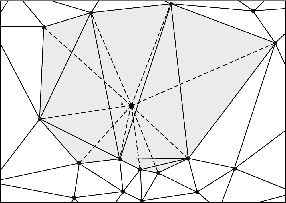
Next, Lemma 2.1 shows that

(4.9)

\text{\rm card\hskip 1.0pt}\mathsf{C}^{+}_{x}(\omega)=\text{\rm card\hskip 1.0pt}\mathsf{C}_{x}(\omega)+2\,,

and for every $\Lambda\ni x$ we have

(4.10)

H_{\Lambda,\omega}(\omega\cup\{x\})-H_{\Lambda,\omega}(\omega)=\sum_{\tau\in\mathsf{C}^{+}_{x}(\omega)}\varphi(\tau)-\sum_{\tau\in\mathsf{C}_{x}(\omega)}\varphi(\tau).

Here is the monotonicity result announced above.

Lemma 4.14

Under the conditions above, there exist a subset $\mathsf{C}_{x}^{\prime}(\omega)\subset\mathsf{C}_{x}(\omega)$ with $\text{\rm card\hskip 1.0pt}\big(\mathsf{C}_{x}(\omega)\setminus\mathsf{C}_{x}^{\prime}(\omega)\big)\leq 4$ and an injection $I$ from $\mathsf{C}_{x}^{\prime}(\omega)$ to $\mathsf{C}^{+}_{x}(\omega)$ such that

(4.11)

\varrho(I(\tau))\leq\varrho(\tau)\hskip 10.00002pt\text{ for all $\tau\in\mathsf{C}_{x}^{\prime}(\omega)$.}

We postpone the proof of this lemma until the end, coming first to its use.

Proof of Proposition 4.13: By assumption, $\varphi$ is eventually increasing. So there exists some $r_{\varphi}<\infty$ and a nondecreasing function $\psi$ such that $\varphi(\tau)=\psi(\varrho(\tau))$ when $\varrho(\tau)\geq r_{\varphi}$ . Combining Lemma 4.14 and Equations (4.9) and (4.10) we thus find that

(4.12)

H_{k,\omega}(\omega\cup\{x\})\leq H_{k,\omega}(\omega)+10\,c_{\varphi}

for all $\omega\in\Omega^{*}$ , $k\geq 1$ , and Lebesgue-almost all $x\in\Lambda_{k}\setminus\omega$ that have at least the distance $2r_{\varphi}$ from all points of $\omega$ . Next, let $P\in\mathscr{G}_{\Theta}(z,\varphi)$ . By definition,

P(N_{k}=0|\mathcal{F}_{\Lambda_{k}^{c}})(\omega)=Z_{k,z,\omega}^{-1}\,e^{-zv_{k}}\,e^{-H_{k,\omega}(\emptyset)}

for all $\omega\in\Omega^{*}$ . Let $\Lambda_{k}^{(2)}=\big\{(x,y)\in\Lambda_{k-2r_{\varphi}}^{2}:|x-y|\geq 2r_{\varphi}\big\}$ . Applying (4.12) twice (viz. to $\omega_{\Lambda_{k}^{c}}$ and $x$ as well as $\omega_{\Lambda_{k}^{c}}\cup\{x\}$ and $y$ ) and recalling (3.2) we find that

\begin{split}Z_{k,z,\omega}&\geq e^{-zv_{k}}\,\frac{z^{2}}{2}\int_{\Lambda_{k}^{(2)}}e^{-H_{k,\omega}(\{x\}\cup\{y\})}\,dx\,dy\\ &\geq{z^{2}\,|\Lambda_{k}^{(2)}|}\,e^{-zv_{k}}\,e^{-H_{k,\omega}(\emptyset)-20\,c_{\varphi}}/\,2\,.\end{split}

Since $|\Lambda_{k}^{(2)}|\sim v_{k}^{2}$ as $k\to\infty$ , the result follows. $\Diamond$

Finally we turn to the proof of Lemma 4.14.

Proof of Lemma 4.14: Let $\tau_{x}$ be the unique triangle of $\mathsf{C}_{x}(\omega)$ containing $x$ in its interior, and $\mathsf{C}_{x}^{+\wedge}(\omega)$ the set of all $\tau\in\mathsf{C}_{x}^{+}(\omega)$ that have an acute or right angle at $x$ . Note that $\text{\rm card\hskip 1.0pt}(\mathsf{C}_{x}^{+}(\omega)\setminus\mathsf{C}_{x}^{+\wedge}(\omega))\leq 3$ because the angles at $x$ of all $\tau\in\mathsf{C}_{x}^{+}(\omega)$ add up to 360 degrees. We will associate to each triangle $\tau\in\mathsf{C}_{x}(\omega)$ a triangle $I(\tau)\in\mathsf{C}^{+}_{x}(\omega)$ , except possibly when $\tau=\tau_{x}$ or the candidate for $I(\tau)$ does not belong to $\mathsf{C}_{x}^{+\wedge}(\omega)$ . Our definition of $I(\tau)$ depends on the number $k=k(\tau)$ of edges $e\subset\tau$ with $\langle e\rangle\subset\partial\Delta_{x}(\omega)$ . Let $\mathsf{C}^{(k)}_{x}(\omega)$ be the set of all $\tau\in\mathsf{C}_{x}(\omega)$ that have $k$ such edges. Since $\mathsf{C}^{(3)}_{x}(\omega)=\emptyset$ except when $\mathsf{C}_{x}(\omega)=\{\tau_{x}\}$ , we only need to consider the three cases $k=0,1,2$ .

The cases $k=1$ and $2$ are easy: For every $\tau\in\mathsf{C}^{(1)}_{x}(\omega)$ there exists a unique edge $e(\tau)$ such that $e(\tau)\cup\{x\}\in\mathsf{C}_{x}^{+}(\omega)$ . If in fact $e(\tau)\cup\{x\}\in\mathsf{C}_{x}^{+\wedge}(\omega)$ we set $I(\tau)=e(\tau)\cup\{x\}$ ; otherwise we leave $I(\tau)$ undefined. Likewise, every $\tau\in\mathsf{C}^{(2)}_{x}(\omega)$ has two edges $e_{1}(\tau)$ and $e_{2}(\tau)$ in $\partial\Delta_{x}(\omega)$ (in clockwise order, say) and can be mapped to $I(\tau)=e_{1}(\tau)\cup\{x\}$ , provided this triangle belongs to $\mathsf{C}^{+\wedge}_{x}(\omega)$ . The resulting mapping $I$ is clearly injective. Moreover, $\tau$ and $I(\tau)$ have the edge $e(\tau)$ (resp. $e_{1}(\tau)$ ) in common, and $x\in B(\tau)$ because $\tau\in\mathsf{C}_{x}(\omega)$ . Since $I(\tau)\in\mathsf{C}^{+\wedge}_{x}(\omega)$ whenever it is defined, we can conclude that $\varrho(I(\tau))\leq\varrho(\tau)$ .

The case $k=0$ is more complicated because the tiles $\tau\in\mathsf{C}^{(0)}_{x}(\omega)$ are not naturally associated to a tile of $\mathsf{C}^{+}_{x}(\omega)$ . To circumvent this difficulty we define an injection $\tilde{I}$ from $\mathsf{C}^{(0)}_{x}(\omega)\setminus\{\tau_{x}\}$ to $\mathsf{C}^{(2)}_{x}(\omega)$ such that $\varrho(\tilde{I}(\tau))\leq\varrho(\tau)$ . Each triangle $\tau\in\mathsf{C}^{(0)}_{x}(\omega)$ different from $\tau_{x}$ can then be mapped to the triangle $I(\tau)=e_{2}(\tilde{I}(\tau))\cup\{x\}$ , provided the latter belongs to $\mathsf{C}_{x}^{+\wedge}(\omega)$ ; otherwise $I(\tau)$ remains undefined. This completes the construction of $I$ . (Note that $\tau_{x}$ does not necessarily belong to $\mathsf{C}^{(0)}_{x}(\omega)$ . However, if it does we have no useful definition of $\tilde{I}(\tau_{x})$ .)

To construct $\tilde{I}$ we turn $\mathsf{C}_{x}(\omega)$ into the vertex set of a graph $G_{x}(\omega)$ by saying that two tiles are adjacent if they share an edge. The set $\mathsf{C}^{(2)}_{x}(\omega)$ then coincides with the set of all leaves of $G_{x}(\omega)$ , and $\mathsf{C}^{(0)}_{x}(\omega)$ is the set of all triple points of $G_{x}(\omega)$ .

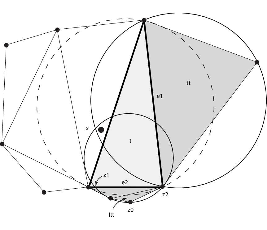
Consider a fixed $\tau_{*}\in\mathsf{C}^{(0)}_{x}(\omega)\setminus\{\tau_{x}\}$ . Since $\tau_{*}\subset\partial\Delta_{x}(\omega)$ , the set $\Delta_{x}(\omega)\setminus\langle\tau_{*}\rangle$ splits into three connected components. Let $W_{i}=W_{i}(\tau_{*},x,\omega)$ be the closure of the $i$ th component, $i=1,2,3$ . Any two of these sets intersect at a point of $\tau_{*}$ , and one of them contains $x$ because $\tau_{*}\neq\tau_{x}$ . Suppose $x\in W_{3}$ . For $i=1,2$ let $e_{i}=\tau_{*}\cap W_{i}$ be the edge of $\tau_{*}$ that separates $W_{i}$ from the rest of $\Delta_{x}(\omega)$ ; see Fig. 2. We claim that there exists some $i=i(\tau_{*})\in\{1,2\}$ such that

(4.13)

\varrho(\tau)\leq\varrho(\tau_{*})\hskip 10.00002pt\text{ for all $\tau\in\mathsf{C}_{x}(\omega)$ with $\tau\subset W_{i}$}\,.

The image $\tilde{I}(\tau_{*})$ of $\tau_{*}$ can then be defined as the leaf of $G_{x}(\omega)$ in $W_{i(\tau_{*})}$ with the largest circumcircle. (The largest circumcircle condition takes account of the fact that the path in $G_{x}(\omega)$ from $\tau_{*}$ to $\tilde{I}(\tau_{*})$ might contain further triple points.)

It remains to prove (4.13). Since $\tau_{*}\neq\tau_{x}$ , there exists at least one $i$ such that the triangle $\{x\}\cup e_{i}$ has an acute angle at $x$ . We fix such an $i$ and consider any $\tau\in\mathsf{C}_{x}(\omega)$ with $\tau\subset W_{i}$ . There exists at least one point $z_{0}\in\tau$ that is not contained in the closed disc $\overline{B}(\tau_{*})$ . Since $x\in B(\tau)$ and $\langle\tau\rangle$ is covered by the tiles $\langle\tau^{\prime}\rangle$ for $\tau^{\prime}\in\mathsf{C}^{+}_{x}(\omega)$ with $\langle\tau^{\prime}\rangle\cap\langle e_{i}\rangle\neq\emptyset$ , we conclude that the line segment $s$ from $z_{0}$ to $x$ is contained in $\overline{B}(\tau)$ and hits both the circle $\partial B(\tau_{*})$ and the edge $\langle e_{i}\rangle$ . In particular, $B(\tau)\cap\langle e_{i}\rangle\neq\emptyset$ . Since $B(\tau)$ contains no points of $\omega$ , we deduce further that the circle $\partial B(\tau)$ hits the edge $\langle e_{i}\rangle$ in precisely two points $z_{1}$ and $z_{2}$ . By the choice of $i$ , the angle of the triangle $\{z_{1},x,z_{2}\}$ at $x$ is acute. Since $x\in B(\tau)$ , it follows that the angle of the triangle $\{z_{1},z_{0},z_{2}\}$ at $z_{0}$ is obtuse. Consequently, if we consider running points $y_{k}$ such that $y_{0}$ runs from $z_{0}$ to the point $s\cap\partial B(\tau_{*})$ and the edge $\{y_{1},y_{2}\}$ from $\{z_{1},z_{2}\}$ to $e_{i}$ , the associated circumcircles $B(\{y_{1},y_{0},y_{2}\})$ run from $B(\tau)$ to $B(\tau_{*})$ , and their radii $\varrho(\{y_{1},y_{0},y_{2}\})$ must grow. This proves that $\varrho(\tau)\leq\varrho(\tau_{*})$ , and the proof of (4.13) and the lemma is complete. $\Diamond$

Acknowledgment. We are grateful to Remy Drouilhet who brought us together and drew the interest of H.-O. G. to the subject.

References

[1] M. Aigner and G. Ziegler, Proofs from the book, Springer, Berlin etc., 3rd ed., 2004.
[2] E. Bertin, J.-M. Billiot and R. Drouilhet, Existence of “nearest-neighbour” spatial Gibbs models, Adv. in Appl. Probab. 31:895–909 (1999)
[3] E. Bertin, J.-M. Billiot and R. Drouilhet, Existence of Delaunay pairwise Gibbs point process with superstable component, J. Statist. Phys. 95:719–744 (1999)
[4] E. Bertin, J.-M. Billiot and R. Drouilhet, Phase transition in the nearest-neighbor continuum Potts model, J. Statist. Phys. 114:79–100 (2004)
[5] E. Bertin, J.-M. Billiot and R. Drouilhet, $R$ -local Delaunay inhibition model, J. Stat. Phys. 132:649–667 (2008)
[6] A. Dembo and O. Zeitouni, Large Deviations: Techniques and Applications. Springer, New York, 1998.
[7] D. Dereudre, Gibbs Delaunay tessellations with geometric hard core conditions, J. Statist. Phys. 131:127–151 (2008).
[8] D. Dereudre, R. Drouilhet and H.-O. Georgii, Existence of Gibbsian graphs for stable interactions, in preparation.
[9] J. Fritz, Generalization of McMillan’s theorem to random set functions. Stud. Sci. Math. Hung. 5:369–394 (1970).
[10] H.O. Georgii, Gibbs Measures and Phase Transitions, de Gruyter, Berlin, 1988.
[11] H.O. Georgii, Large deviations and maximum entropy principle for interacting random fields on ${\rm Z}^{d}$ , Ann. Probab. 21:1845–1875 (1993).
[12] H.O. Georgii, Large deviations and the equivalence of ensembles for Gibbsian particle systems with superstable interaction, Probab. Theory Relat. Fields 99:171–195 (1994).
[13] H.O. Georgii, The equivalence of ensembles for classical systems of particles, J. Statist. Phys. 80:1341-1378 (1995).
[14] H.O. Georgii and H. Zessin, Large deviations and the maximum entropy principle for marked point random fields, Probab. Theory Relat. Fields 96:177–204 (1993).
[15] G. Grimmett, Potts models and random-cluster processes with many-body interactions, J. Statist. Phys. 75:67–121 (1994).
[16] R. Holley and D. W. Stroock, Nearest neighbor birth and death processes on the real line, Acta Math.Ê140:103–154 (1978).
[17] J. Møller, Lectures on Random Voronoi Tessellations, Lecture Notes in Statistics Vol. 87, Springer, Berlin etc., 1994.
[18] X.X. Nguyen and H. Zessin, Ergodic theorems for spatial processes, Z. Wahrscheilichkeitstheor. Verw. Geb. 48:133–158 (1979).
[19] C. Preston, Random fields, Lect. Notes Math. 534, Springer, Berlin, 1976.
[20] R. Schneider and W. Weil, Stochastic and integral geometry, Springer, Berlin, 2008.
[21] H. Zessin, Specific index and curvature for random simplicial complexes, Inst. Math. Natl. Acad. Sci. Armenia 37:64–81 (2002).