UMD-PP-09-039 Higgs Mediated FCNC’s in Warped Extra Dimensions
Abstract
In the context of a warped extra-dimension with Standard Model fields in the bulk, we obtain the general flavor structure of the Higgs couplings to fermions. These couplings will be generically misaligned with respect to the fermion mass matrix, producing large and potentially dangerous flavor changing neutral currents (FCNC’s). As recently pointed out in [arXiv:0906.1542], a similar effect is expected from the point of view of a composite Higgs sector, which corresponds to a 4D theory dual to the 5D setup by the AdS-CFT correspondence. We also point out that the effect is independent of the geographical nature of the Higgs (bulk or brane localized), and specifically that it does not go away as the Higgs is pushed towards the IR boundary. The FCNC’s mediated by a light enough Higgs (specially their contribution to ) could become of comparable size as the ones coming from the exchange of Kaluza-Klein (KK) gluons. Moreover, both sources of flavor violation are complementary since they have inverse dependence on the 5D Yukawa couplings, such that we cannot decouple the flavor violation effects by increasing or decreasing these couplings. We also find that for KK scales of a few TeV, the Higgs couplings to third generation fermions could experience suppressions of up to while the rest of diagonal couplings would suffer much milder corrections. Potential LHC signatures like the Higgs flavor violating decays or , or the exotic top decay channel , are finally addressed.
I Introduction
Introducing a warped extra-dimension in such a way as to create an exponential scale hierarchy between the two boundaries of the extra dimension [1] has generated a lot of attention in the recent years as a novel approach to solve the hierarchy problem. By placing the Standard Model (SM) fermions in the bulk of the extra dimension it was then realized that one can simultaneously address the flavor hierarchy puzzle of the SM [2, 3]. The electroweak precision tests put important bounds on the scale of new physics but by introducing custodial symmetries [4] one can have it around few TeV [4, 5, 6, 7].
In this paper we will study the class of models in which all the SM fields are in the bulk and the hierarchies in masses and mixings in the fermion sector are explained by small overlap integrals between fermion wave functions and the Higgs wave function along the extra dimension. This scenario can lead to the observed fermionic masses without any hierarchies in the initial 5D Lagrangian, so that our fundamental 5D Yukawa couplings have no structure and are all of the same order. Another interesting feature of these models is that the contributions to low energy observables coming from the exchange of heavy KK states will be suppressed by the so called “RS GIM” mechanism [8, 9]. In spite of it, it was still found that processes push the mass of the KK excitations to be above TeV [10, 11, 12, 13], making it very hard to produce and observe them at the LHC [14, 15]. These bounds coming from flavor violation in low energy observables can be avoided by introducing additional flavor symmetries [12, 13, 16, 17]. Another way to relax these low energy constraints is to promote the Higgs to be a 5D bulk field (instead of being brane localized). In this situation the bounds from could allow masses of the lowest KK gluon to be as low as TeV, although combining this result with the bounds from dipole moment operators pushes back the KK scale to be above TeV [18, 19]. A similar tension was found in the lepton sector in [20].
It has recently been pointed out that in the context of a composite Higgs sector of strong dynamics, one generically expects some amount of flavor changing neutral currents (FCNC’s) mediated by the Higgs [21] (from an effective field theory point of view see also the earlier works [22, 23, 24, 25]). In the 5D picture, the presence of KK fermion states will actually produce a misalignment between the Higgs Yukawa couplings and the SM fermion masses, giving rise to tree-level flavor violating couplings of the Higgs to fermions. The induced FCNC’s are strongly constrained by various low energy experiments; if these constraints are somehow evaded, interesting signals at the LHC could also be generated.
The possibility of a flavor misalignment between the Higgs Yukawa matrices and the fermion mass matrices in the context of 5D warped scenarios was first briefly mentioned in [26], although it was not until [27] where a detailed analysis of the flavor structure of the couplings of the Higgs (brane localized) was first performed. There, the effects on the flavor violating Higgs couplings were found to be small (except for third generation quarks), with the (hidden) assumption that the contribution from a specific type of operators is negligible. In a more general Higgs context (bulk or brane localized), all the sources of Higgs flavor violation were then pointed out in [11, 28], including the previously neglected operators, although no analysis on the overall size of the Higgs FCNC’s was performed. Moreover, in the limit of a brane localized Higgs, the effects of the larger sources of flavor are claimed to become negligible, and so it is again found that Higgs mediated FCNC’s are highly suppressed in the case of a brane Higgs.
In this work, we show that the induced misalignment in the Higgs couplings is generically large and phenomenologically important in both bulk and brane localized Higgs scenarios. The main cause for this result is the effect of the originally neglected operators which, due to a subtlety in the treatment of the brane localized Higgs, ends up surviving in the brane limit and giving rise to important misalignments between the Higgs Yukawa couplings and the fermion mass matrices.
The outline of the paper is as follows: in section II we review the model independent argument such that (TeV suppressed) higher order effective operators in the Higgs sector can lead to potentially large Higgs FCNC’s. This is then applied to the 5D RS model, first in the mass insertion approximation in order to quickly estimate the size of the corrections. In section III we proceed with a more precise calculation of the Higgs Yukawa couplings in the case of one fermion generation, and for a bulk Higgs scenario. The deviation in the Yukawa couplings is quite insensitive to how much the Higgs is localized near the IR brane; this result is confirmed in section IV by doing a 5D computation for the case of an exactly IR localized Higgs field, and it seems at odds with the mass insertion approximation which suggests that the corrections to the flavor violating Higgs couplings should vanish in the brane Higgs limit. This apparent contradiction is addressed and resolved in that same section. In section V we extend our results to the case of three generations and then in section VI, we give an estimate of the expected overall size of the Yukawa coupling matrices. We also argue that the couplings of the Higgs to third generation fermions might be significantly suppressed. These estimates are confirmed in section VII by the results of our numerical scan. Finally, section VIII is devoted to the study of phenomenological implications of Higgs mediated flavor violations, where we discuss low energy bounds arising from processes as well as interesting collider signatures.
II Flavor misalignment estimate
From an effective field theory approach it is easy to write the lowest order operators responsible for generating a misalignment in flavor space between the Higgs Yukawa couplings and the SM fermion masses. For simplicity we focus on the down quark sector and write the following dimension 6 operators of the 4D effective Lagrangian [22, 23, 24, 25, 21]:
| (1) |
where and are the fermionic doublets and singlets of the SM, with , and being complex coefficients and are flavor indices; is the cut-off or the threshold scale of the effective Lagrangian. Upon electroweak symmetry breaking (EWSB), these operators will give a correction to the fermion kinetic terms and to the fermion mass terms. Calling the original Yukawa couplings, the corrected fermion mass and kinetic terms become:
| (2) |
where GeV is the Higgs electroweak , i.e. , with being the physical Higgs scalar. On the other hand, the induced operators involving two fermions and one physical Higgs become:
| (3) |
From Eq.(2) it is clear that one has to redefine the fermion fields to canonically normalize the new kinetic terms and then perform a bi-unitary transformation to diagonalize the resulting mass matrix. These fermion redefinitions and rotations will not in general diagonalize the couplings from Eq. (3) and therefore, we will obtain tree-level flavor changing Higgs couplings, with a generic size controlled by .
In the warped extra dimensions scenarios that we are interested in, we can estimate easily the size of this type of misalignments between the Higgs Yukawa couplings and the SM fermion masses by using the insertion approximation in KK language. The 5D spacetime we consider takes the usual Randall-Sundrum form [1]:
| (4) |
with the UV (IR) branes localized at () and with being the curvature scale of the AdS space. We are interested here in the flavor structure of the Yukawa couplings between the Higgs and the fermions. However, it is instructive to first consider the case of only one generation and study the (potentially large) corrections induced to the single Yukawa coupling. One can then easily generalize to three generations and find the misalignment between the fermion mass matrix and the Yukawa couplings matrix.
We will focus on the down-quark sector of a simple setup in which we consider the 5D fermions , . They contain the 4D SM doublet and singlet fermions respectively with a 5D action
| (5) |
where and are the 5D fermion mass coefficients and is the bulk Higgs field localized towards IR brane. The wavefunctions of the fermion zero modes are determined by their corresponding 5D mass coefficients. To obtain a chiral spectrum, we choose the following boundary conditions for
| (6) |
Then, only and will have zero modes, with wavefunctions:
| (7) | |||||
| (8) |
where we have defined and the hierarchically small parameter , which is generally referred to as the “warp factor”. Thus, if we choose , then the zero modes wavefunctions are localized towards the UV brane; if , they are localized towards the IR brane. The wavefunctions of the KK modes are all localized near the IR brane. Note that the wavefunctions of the KK modes and vanish at the IR brane due to their boundary conditions. The Yukawa couplings of the Higgs with fermions (zero modes or heavy KK modes) are set by the overlap integrals of the corresponding wavefunctions. For a bulk Higgs localized near the IR brane, the zero-zero-Higgs, zero-KK-Higgs, KK-KK-Higgs Yukawa couplings are given approximately by
| (9) | |||||
| (10) | |||||
| (11) |
where is the dimensionless 5D Yukawa coupling, and we ignored factors in the equations above. The SM fermions are mostly zero mode fermions with some small amount of mixing with KK mode fermions. Therefore, we can use the mass insertion approximation to calculate the masses and Yukawa couplings of SM fermions. This is shown in Fig. 1, where , are zero modes of doublet and singlet fermions respectively and , , , are KK mode fermions. From the Feynman diagram in Fig. 1 we see that the SM fermion mass is given by

| (12) | |||||
where is the Higgs vev and we assume that all KK fermion masses are of the same order ().
The 4D effective Yukawa couplings of SM fermions can be calculated using the same diagram. However in the second diagram of Fig. 1, we have to set two external to their vev while the other one becomes the physical Higgs , and there are three different ways to do this. Thus we obtain the 4D Yukawa couplings
| (13) |
We see that the SM fermion masses and the 4D Yukawa couplings are not universally proportional; indeed there is a shift with respect to the SM prediction of .
We thus define the shift as
| (14) |
and it is easy to see that the contribution of the diagrams of Fig. 1 to is
| (15) |

There is yet another source of shift between masses and Yukawa couplings coming this time from the corrections to the kinetic terms. This is the contribution which was pointed out and carefully computed in [27], and as wee will see later, in agreement with our own results for that specific term. As shown in Fig. 2, the kinetic term for the fermion mode receives a correction induced by the mixing with KK fermion modes
| (16) |
After redefining fields so that their kinetic term is canonical, there will be a new contribution to the shift between masses and Yukawa couplings given by
| (17) |
Similarly, the correction to the kinetic term of gives the contribution
| (18) |
Adding all terms together, we find the total fermion mass-Yukawa shift
| (19) |
If we extend to the case of three generations, we can see that this shift between SM fermion masses and Yukawa couplings produces a misalignment in flavor space between these. This misalignment will lead to flavor violating Higgs couplings once the fermion mass matrix is diagonalized.
For the first two generation quarks, we need to reproduce their small masses. Therefore, for these first two generations, the shift coming from the correction to kinetic terms (Fig. 2) is negligible and the correction coming from the diagrams in Fig. 1 will dominate. However, for the third generation, all effects are comparable. It is interesting to point out that the expression (Eq. 19) (valid for one generation) is always positive, which leads to a reduction in the 4d effective Yukawa couplings compared to the SM ones.
II.1 Brane Higgs subtlety
Finally, we must mention that there is a subtlety in the case of an exactly brane localized Higgs. As pointed out in [11, 28], since the wavefunctions of and vanish at TeV brane (due to Dirichlet boundary conditions), their couplings to a brane localized Higgs should also vanish. This means that the second diagram in Fig. 1 should give no contribution to the fermion mass-Yukawa shift (or at best a highly suppressed one). We would then expect to be left with only the correction coming from the kinetic term (Fig. 2), which as stated above is negligible for light quarks. We observe, however, that upon EWSB, the wavefunctions and become discontinuous at the brane location [32], with the jump of the wavefunctions being proportional to the brane Higgs vev . This discontinuity requires some sort of regularization of the brane location, meaning that the couplings of and with the brane Higgs would be infinitesimally small, but non-zero. But we note that in the second diagram of Fig. 1, one has to sum over infinite KK modes and even though each KK mode will give an infinitesimally small contribution, the sum of infinite terms can lead to a finite (non-zero) result (and as it turns out, this is what happens, as shown explicitly in Appendix C for this mass insertion approximation).
This brane Higgs issue is avoided in [27] because the authors did not include in their brane action any operator of the type . By avoiding these, the contribution to the shift coming from the diagrams of Fig. 1 is simply not present (except for highly suppressed corrections of order which are safe to ignore).
III 5D calculation: Bulk Higgs Scenario
In this section we perform a 5D calculation in order to evaluate more precisely the shift between Yukawa couplings and masses of SM fermions. We start by working with a single fermion generation for clarity but will later extend our results to the three generations case.
To proceed, we will need to solve for the wavefunctions of SM fermions along the fifth dimension in the bulk Higgs [33, 34] scenario. This corresponds to including the contribution of all KK modes of the mass insertion approximation, and not just the lightest ones. As we will see, the most important shift does not go away as we push the Higgs profile towards the IR brane. In the bulk Higgs scenario, the Higgs comes from a 5D scalar with the following action [33]
| (20) |
where is the 5D mass for Higgs in unit of . The boundary potentials and give the boundary conditions for the Higgs wavefunction. We can choose these boundary conditions such that the profile of the Higgs vev takes the simple form
| (21) |
where and
| (22) |
where is the SM Higgs vev. This nontrivial vev is localized towards the IR brane solving the Planck-weak hierarchy problem. Nevertheless we will treat the brane Higgs case separately later to review possible subtleties inherent to its localization by a Dirac delta function.
After writing the 5D fermions in two component notation, and , we perform a “mixed” KK decomposition as
| (23) | |||||
| (24) | |||||
| (25) | |||||
| (26) |
where correspond to the light 4D SM fermions and the include the rest of heavy KK fermion fields. are the corresponding profiles of the 4D SM fermions and which verify the Dirac equation
| (27) | |||||
| (28) |
with being the 4D SM down-type quark mass (the analysis can be carried out for up-type quarks in similar fashion).
The four profiles and must verify the coupled equations coming from the equations of motion.
| (29) | |||
| (30) | |||
| (31) | |||
| (32) |
where the ′ denotes derivative with respect to the extra coordinate and is 5D Yukawa coupling. Even if one knows the analytical form of the nontrivial Higgs vev , solving analytically this system of equations might still be quite hard. Nevertheless it is simple to find the misalignment between Higgs Yukawa couplings and fermion masses based on the previous equations. To proceed, let us first multiply Eq. (29) by and the conjugate of Eq. (30) by , and then subtract them. One obtains
| (33) |
We can now multiply by and integrate the whole expression between and and obtain
| (34) |
The boundary conditions for the profile are chosen to be Dirichlet at both boundaries, i.e. , which means that the last term of Eq. (34) identically vanishes. Moreover, canonical normalization of the SM d-quark imposes the extra constraint
| (35) |
We can therefore rewrite Eq. (34) as
| (36) |
Note that this identity is exact, but also that each profile and depend on the mass . In the zero mode approximation, the profiles with Dirichlet boundary conditions, and vanish, and the identity can be expressed as
| (37) |
which agrees with the intuition that fermion mass is mostly generated by the 5D Yukawa couplings between the 5D Higgs and the zero mode fermion profiles. From the action in Eq. (5) we also extract the 4D Yukawa coupling of the Higgs field (the lightest KK mode of the 5D Higgs) and the SM down type quark.
| (38) |
where is the profile of the physical Higgs field. It is easy to show that the Higgs vev solution is related to the profile of the physical light Higgs (lightest KK mode) by
| (39) |
so for a light enough Higgs field both profiles and are proportional to each other. For a moderately heavy physical Higgs, there will be a misalignment between the profiles of the Higgs vev and the physical Higgs, leading to a misalignment between fermion masses and Yukawa couplings. However, this effect can actually be decoupled if the Higgs is pushed towards the IR brane (by increasing the parameter ). In this case, the Higgs vev profile will be more and more aligned with that of the physical Higgs, so that they become identical in the brane Higgs limit. This source of Higgs flavor violating couplings will be controlled by the parameter and for the sake of clarity we will ignore its effects in the rest of the paper because, as we discuss in Appendix B, they are numerically small and can be decoupled by pushing the Higgs towards the IR brane.
We can then compute the shift between the fermion mass and the Yukawa coupling as
| (40) |
This identity shows that the shift has to be relatively small since it vanishes in the zero mode approximation.
To proceed further, we will use a perturbative approach such that we assume that where is the SM Higgs vev. Thus, once we know the analytical form of the vev profile (see Eq. (21)) we can solve perturbatively the system of coupled equations (29-32)11 1 It would be interesting to use this perturbative technique in the context of fermion flavor in soft-wall scenarios [29, 30, 31] given that the setup is quite similar; we will leave this analysis for future studies..
We find
| (41) | |||||
| (42) |
and
| (43) | |||||
| (44) |
with the constants and fixed by canonical normalization of the kinetic terms giving
| (45) | |||||
| (46) |
Equipped with the solutions from Eqs. (41) to (44) one can evaluate perturbatively the shift defined in Eq. (40). For simplicity, we present here the results for UV localized fermions (). The general results for both UV and IR localized fermions are presented in Appendix A. We find that the main contribution to the shift coming from the last term in Eq. (40) can be written as
| (47) |
This result corresponds to the one we estimated earlier by using the insertion approximation (see Eq. (15)).
The first term in Eq. (40) gives a subleading contribution to the shift
| (48) |
which corresponds to the one coming from the kinetic correction using the insertion approximation (Eq. 17 and 18).
Even if the fermion mass is small, the large warp factor will overcome most of the suppression, rendering the shift to be of the order . The shift is generally on the percent level with respect to fermion masses, but a misalignment of this order in the Higgs Yukawa couplings should introduce strong constraints due to FCNC’s.
III.1 Pushing the Higgs from the bulk to the brane
Note that in the limit, the profile of the Higgs vev tends to become brane localized, as well as the light physical Higgs and the rest of Higgs KK modes. In this limit, the shift produced between the fermion mass and the Yukawa coupling, coming from the diagrams of Fig. 1, reduces to
| (49) |
and in particular we see that the effect does not decouple (i.e. it is non-zero). The fact that the expected misalignment is more or less independent on the localization of the Higgs is one of our main results since the bounds and predictions that we will extract can then be considered a general feature of RS models with fields in the bulk (and a Higgs scalar localized near or at IR brane)22 2 An interesting exception to these results in the Higgs sector, proposed in [21], would be to eliminate the Higgs as a fundamental scalar and consider the fifth component of a gauge field as playing the Higgs role in EWSB.. The shift coming from the corrections to the fermion kinetic terms (Fig. 2) becomes in the limit
| (50) |
in agreement with the results found in [27] (for a brane Higgs scenario).
Maybe it can be useful to discuss the validity of the limit starting from a bulk Higgs scenario. Let’s first look at the mass spectrum in this case. The Higgs profile is given by Eq. (129) and to find its mass eigenvalues one has to satisfy the appropriate boundary conditions at the IR brane [33]
| (51) |
This will lead to one light mode (i.e. SM Higgs) and a tower of heavy modes with masses proportional to , and so in the limit all the KK Higgs excitations are decoupled from the low energy spectrum. This means that in this limit we can treat Higgs field as an effective four dimensional field, and thus it corresponds to the brane Higgs scenario. As mentioned earlier (and in Appendix B), the misalignment caused by a difference in profiles between the Higgs physical field and its vev (and which we have neglected) will also disappear, as one can interpret that specific misalignment as a result of the mixing between SM Higgs and the heavy Higgs KK modes, which is controlled by .
Let us now look on the couplings of fermions to the Higgs in this limit. For the zero modes we will get:
| (52) |
where ; similarly one can look at the couplings of two KK fermions to the Higgs and in this case one finds its dependence to be . Naively both couplings do vanish in the limit. But if the 5D couplings scale as then these couplings will have a finite limit given by the usual brane Higgs results. One can argue whether we can scale the 5D Yukawas as because such large Yukawas should violate perturbativity of the theory, but as was shown above the couplings of the Higgs to the KK fermions are still . One can see that only the KK excitations of the Higgs will have couplings with KK fermions , but their masses are and they are completely decoupled from the spectrum. So we conclude this discussion by stressing that it is consistent to consider the limit with and it coincides with the usual brane Higgs scenario.
IV 5D calculation: Brane Higgs Scenario
We argued in Section II that one might expect that the major contribution to the misalignment vanishes in the brane Higgs case since the odd KK modes , have vanishing wavefunctions on the IR brane. We also briefly mentioned that in the mass insertion approximation, one actually might need to sum the infinite tower of fermion KK modes to obtain a non-vanishing contribution (see Appendix C for details). However, without invoking that explanation, we just saw that in the limit, approaches a nonzero value of same numerical order as the case. Since the limit of bulk Higgs corresponds to a brane localized Higgs, there seems to be a counter-intuitive subtlety. In this section we try to address and resolve this point in a more precise way, by performing the 5D calculation of the shift for the specific scenario of a brane Higgs.
For brane Higgs, we can write the Yukawa couplings in the Lagrangian as
| (53) |
Here we choose the convention with . Note that compared to the bulk Higgs case, the Yukawa couplings an are independent and both . However, they should be of the same order due to the philosophy of flavor anarchy and naturalness. We can do KK decomposition as before, then the equations satisfied by the wavefunctions are
| (54) | |||
| (55) | |||
| (56) | |||
| (57) |
Notice that the odd wavefunctions and vanish at the IR brane. But the delta functions in equations above give a jump for and at the IR brane, which makes their values at IR brane ambiguous [32]. To remove this ambiguity, we “regularize” the delta in the following way
| (58) |
This regularization is in a way similar to treating the Higgs as a bulk field and then taking the limit , although without apparent divergences coming from taking to be large. In any case one could also perform other regularization methods to remove the wavefunction ambiguities at the IR brane33 3 For example, we could have chosen instead to move the delta function location from to , and enforce the usual boundary conditions on the fields at . Then, at the very end, we would take the limit [32]. In that case we find (59) where we have used the step function for and for . Inserting this into Eq. (40) we obtain the same misalignment as in Eq. (65), namely .
Now we can easily impose Dirichlet boundary conditions for the profiles at IR brane
| (60) |
Integrating equations of motion (Eq. 54) from () will lead to
| (61) | |||||
| (62) |
For the rectangular potential profiles will drop to zero linearly in the region , so the profiles near the IR brane can be approximated by
| (63) | |||
| (64) |
From our previous discussion, the main contribution to the misalignment between SM fermion masses and Yukawa couplings come from the second term of Eq.( 40), so plugging in the odd wavefunctions from Eq.(63), we get
| (65) | |||||
On the other hand, to leading order in Higgs vev, the SM fermion mass is given by
| (66) |
Therefore, the misalignment can be expressed as
| (67) |
As advertised before, this result agrees with the one obtained in the previous section for the bulk Higgs scenario, once we take (Eq. 47). We again stress that this result shows that upon careful derivation, the misalignment obtained does not vanish in the particular case of a Brane localized Higgs. The main difference though, is the appearance of the independent couplings , which in the bulk Higgs case are forced to be equal to by 5D general covariance. These couplings are not necessary for generating fermion masses, and so it is technically possible to set their values as small as necessary to suppress the obtained misalignment. Nevertheless this seems to go against the main philosophy of our approach which is to assume the value of all dimensionless 5D parameters of order one.
Again, the fact that is non zero in the brane Higgs case is hard to understand in the mass insertion approximation since the contribution from each KK fermion (see Fig. 1) seems to be vanishing. In Appendix C we show that to resolve this point we need to sum up all the KK modes of the mass insertion approximation, as already mentioned before.
The subleading contribution to the misalignment between SM fermion masses and Yukawa coupling can be calculated in a similar way as in the previous section, and the result is (for UV localized fermions)
| (68) | |||||
| (69) |
We can see that for the first two generations, we have , and it agrees with Eq. (48) in the limit. The result for both UV and IR localized fermions is given by
| (70) |
with
| (71) |
One can see that and can be of the same order only for IR localized fermions.
V Generalizing to three Generations
We can generalize the calculations presented in the sections III and IV to 3 generations. For simplicity we perform the analysis in the brane Higgs scenario here. To leading order in Yukawa, the SM fermion mass matrix is
| (72) |
where means a matrix in flavor space and . Using the same technique as before, we can easily show that the misalignment between fermion mass and Yukawa coupling matrix is , with
| (73) | |||||
| (74) |
and
| (75) |
The subdominant contribution here (Eq. 75) agrees with the result found in [27]. The crucial observation is that and are generally not aligned in flavor space. Thus when we diagonalize the quark mass matrix with a bi-unitary transformation , the Yukawa couplings will not be diagonal. To be more specific, in models of flavor anarchy, we have
| (76) |
Then the off-diagonal Yukawa coupling will be (dominated by Eq. (73))
| (77) | |||||
where is the typical value of the dimensionless 5D Yukawa coupling.
VI Estimates of Higgs FCNC in Flavor Anarchy
In this section, we estimate the off-diagonal couplings of Higgs to SM fermions (assuming again for simplicity a brane Higgs scenario). And then we do a numerical scan over anarchical Yukawa couplings to support our estimates. We first parametrize the Higgs Yukawa couplings as
| (78) |
We can use Eq. (76) and (77) to estimate the sizes of . For example, we have
| (79) | |||||
where is the Wolfenstein parameter, and we used . We can find the other ’s in similar fashion. Here we present our results from estimates:
Note that the results we presented here are just estimates for the size of , not their signs or phases. However, for the third generation quarks, the corrections almost always suppress the Yukawa couplings if (which is natural in bulk Higgs scenario) and are typically larger than the previous estimates. We argue this point in the next subsection.
VI.1 Yukawa couplings of the third generation when
We can obtain a better estimate on the typical size of the diagonal entries of the Yukawa coupling matrices by going back to Eq. (74) and assume that . Its form simplifies further to
| (88) |
where we have written the misalignment in the up-sector. Now we perform the bi-unitary rotation needed to go to the physical fermion basis, and study the element (33) of the overall Yukawa coupling, i.e.
| (89) | |||||
First let’s look at the contribution to when the “” index is equal to 3 (i.e. in the middle mass matrix we have ). In this case, there will be 9 terms, each proportional to , and it is important to realize that every one of them will be real and negative, because . When there will be only 4 terms but every one of them will have generically a random complex phase (the 5 remaining terms are much smaller). For there is only one term contributing, with the other 8 terms being again suppressed. So at the end of the day the dominant contribution to will consist of 14 terms, 9 of which are negative and the rest 5 have random complex phases. Generically each of these terms are of the same size so from a statistical argument, should receive a negative contribution . This result is confirmed by the numerical scan presented below.
One can perform the same analysis for the element (22) of the Yukawa matrix and realize that in this case the number of terms aligned (contributing constructively) is 4, and for the (11) element there are none. This means that the largest corrections are expected in the third generation Yukawa couplings, with a suppressed correction in second generation couplings and much more suppressed correction for first generation couplings. This structure in the corrections seems to be a result of the hierarchical structure of the flavor anarchy setup.
Finally, we must remind the reader that it was crucial to take (which is required in the Bulk Higgs scenario) to obtain these predictions. In the case , there will be no alignment of terms, and we therefore generally expect smaller corrections to the third generation Yukawa couplings.
VI.2 Validity of expansion
We managed to solve the fermion equations by expanding them in the parameter , and so our results can be trusted as long as
| (90) |
but we have seen in the previous subsection that the corrections to and couplings do pick up an extra numerical factor of in the expansion parameter . This means that, at least for third generation fermions, our approximation is valid only for
| (91) |
Generically for the case with we will still have a large misalignment between the Higgs couplings and fermion masses but to be able to make valid predictions one would have to solve the equations of motion (Eq. 29 to 32) exactly or use a different perturbative parameter. In the numerical analysis presented below we performed a scan with , where our expansion is valid. We then also allowed for slightly larger values of the Yukawas such that . The average size of the couplings is still below , so for a KK scale of GeV or above, the results will still be precise enough, although approaching the edge of perturbative convergence.
VI.3 Numerical Scan
We did a numerical scan over the input parameters , , , , and we set TeV. In our scan, we pick the points that give the correct SM quark masses and CKM matrix. Then we calculate the 4D effective Yukawa couplings of Higgs with SM quarks. We present here only the results for . First, we scan the set of parameters with which is motivated by bulk Higgs. Here are the results for this case:
The first and second numbers are the and quantiles of the distribution of obtained from the scan (i.e. of all the values we obtained in the scan for each lie between these two quantiles). From the results we can see that the values of from the scan are consistent with the estimates presented above (Eq VI and VI), and the expected reduction of coupling is confirmed. We can also easily see this reduction of third generation Yukawa couplings in Fig. 3.
For the case when and are completely uncorrelated (Brane Higgs) we get the following results:
We can see that the off-diagonal terms of are of the same order as the previous case. However the diagonal entries do not have the suppression as in the case, see the discussion in Subsection VI.1.


VII Lepton sector
Generically one can see that the same effects will lead to Higgs flavor violation in the lepton sector, the only difference is that in the lepton sector there are various ways to explain the large mixing angles and light masses for the neutrinos [35, 36, 37]. Now we want to look at Higgs flavor violation in the charged lepton sector, then depending on a given neutrino model, the left-handed charged lepton profiles can be either hierarchical and UV localized (i), or similar and UV localized (ii). The profiles of the right-handed charged leptons are always hierarchical and localized near the UV brane. We treat these two cases separately.
- •
Case (i) - left-handed and right-handed profiles are hierarchical. Then the profiles should satisfy the following relations:
(108) where are profiles of the left-handed and right-handed fields respectively, then the generational mixing is also hierarchical
(109) We again parameterize our Lagrangian in the following form:
(110) Where are doublets and singlets respectively Then we can estimate
(111) One can see that our estimate depends on the profiles of the fermions, but the following relation will be valid
(112) This inequality is saturated when , i.e., when the hierarchy of charged lepton masses are explained equally by the profiles of left-handed and right-handed fields.
- •
Case (ii) - right-handed profiles are hierarchical and left-handed profiles are similar . Then the profiles satisfy the following relations:
(113) then we can estimate the parameter to be:
(114) These flavor violating Higgs Yukawa couplings to leptons can also lead to interesting collider signals, which will also be discussed in the next section.
VIII Phenomenology
The FCNC generated by flavor violating Higgs Yukawa couplings will affect many low energy observables and also give possible signature at colliders. In this section, we first discuss bounds on Higgs flavor violation coming from processes such as , , mixing. And then we discuss possible signature at the LHC including suppression of coupling, rare top decay and flavor violating Higgs decay .
VIII.1 Bounds from low energy physics

The process can be described by the general Hamiltonian [38, 39]
| (115) |
with
| (116) | |||||
where are color indices. The operators are obtained from by exchange . For , , , mixing, , , and respectively. Exchange of the Higgs can give rise to new contribution to , and . This can be seen in Fig. 4, where Fig. 4(A) gives and , Fig. 4(B) gives . These new contributions are
| (117) | |||||
| (118) | |||||
| (119) |
where is the mass of physical Higgs. The model independent bound on the new physics contribution to these Wilson coefficients are given in [38]. We use the RGE from [40] and give the bounds renormalized at the scale :
| (120) | |||
| (121) | |||
| (122) | |||
| (123) |
These bounds put constraints on both the Higgs flavor violating Yukawa couplings parametrized by , and on the Higgs mass . If we assume that the phases of are random, i.e., , we can then rewrite the previous bounds as
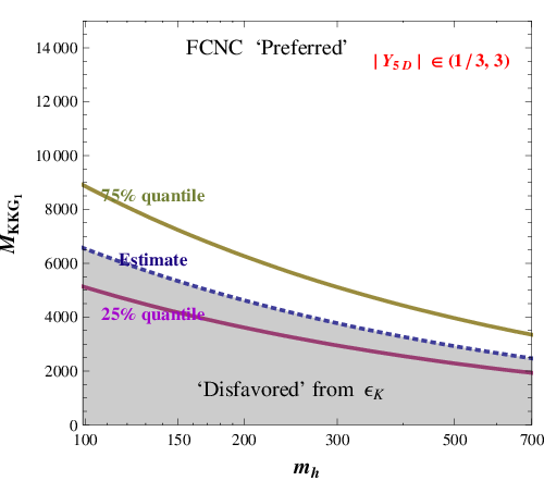
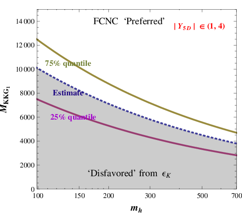
where we compare the elements with their estimated values, for a fixed average Yukawa coupling and KK scale given by GeV (see formulae for the estimates from Eqs. (VI) and (VI) ). We also choose to compare the Higgs mass with a nominal value of GeV. We can see that the bound on coming from gives the strongest constraint on the Higgs mass. Specifically, we have
| (124) |
for a fixed KK scale of TeV and average 5D Yukawa of .
In Fig.5, we show the results of our numerical scan by plotting the bounds coming from in the (-) plane, where is the mass of the first KK gluon. In the left panel we show results for the case , and in the right panel we show results for the case . It can be seen quite clearly that a larger 5D Yukawa coupling leads to a higher bound on the KK scale. Note that the bounds coming from KK gluon exchange are inversely proportional to the size of the 5D Yukawa couplings . This leads to an interesting observation
- •
The new contribution to coming from Higgs exchange has opposite dependence on the 5D Yukawa coupling as that of KK gluon exchange. Thus, increasing the overall size of will alleviate pressure from KK gluon exchange but, as we have seen, this will also enhance the effect of Higgs mediated FCNC’s.
With the chosen (), we can see that for the region of parameter space with TeV (accessible at the LHC), a Higgs mass GeV is disfavored. On the other hand, if a light ( GeV) Higgs is found in the LHC, we should expect sizable new physics contributions to processes, just below current bounds.
VIII.2 Collider phenomenology
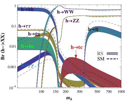
Besides low energy physics constraints, there could be very interesting signatures in colliders coming from the corrections to the Higgs Yukawa couplings. First of all, the reduction in the coupling, as argued in Section VI.1 and confirmed by our numerical scan, tells us that the Higgs production through gluon fusion will be generically suppressed (at least for the bulk Higgs scenario). This coupling can easily be suppressed by (for TeV and ), and therefore the cross section will experience a reduction of with respect to the expected SM value. This reduction in Higgs events from gluon fusion at the LHC can be observed quite clearly as well as the relative increase in importance of the production through gauge boson fusion [41]. We note again that the expected suppression is much larger in the case of a bulk Higgs, namely when we have . In the case where and are unrelated, but with same overall size, there will not be a definitive prediction on the sign of the correction to the top Yukawa and bottom Yukawa couplings (i.e. there could be also enhancements), although the size of the corrections is expected to be smaller than in the case.
In the case of a light Higgs boson (and assuming that somehow low energy FCNC bounds are overcome), the branchings of the Higgs can change substantially due to the generically reduced couplings. This would indirectly enhance the importance of signal, and maybe help overcome the overall reduction in the total production cross section due to reduced top Yukawa couplings. In Fig. 6, we plot the Higgs decay branching ratio for various final states versus the Higgs mass 44 4 We did not include mode on the plot because it is model dependent.. We can see clearly that for a light Higgs, the reduction in the coupling changes the branching ratio to other channels significantly. For a heavy Higgs, the branching for is reduced.
If kinematically accessible (), the flavor violating couplings will allow the decay to occur. The branching ratio of this process is given by (see for example [27])
| (125) |
If we take GeV, then for and , which are good estimates for and a KK scale of GeV (see Eq. (VI)), we obtain a branching ratio of
| (126) |
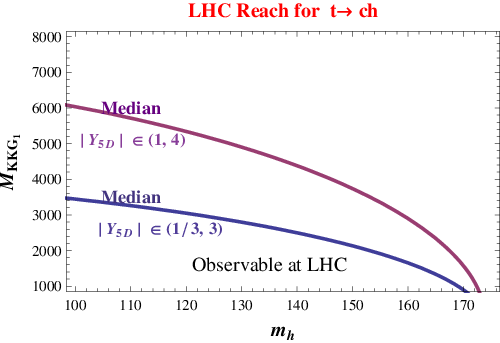
The sensitivity of LHC for this rare top decay is [42], precisely in the ball-park of our estimate. In Figure 7 we show the results of our two scans, each with a different average size of the 5D Yukawas. It is shown that observing the signal at the LHC is quite possible although it requires larger Yukawa couplings and a light Higgs. If observed, this signal would be very valuable in determining the structure of the 5D setup.
Another interesting collider signature for light Higgs might be the Higgs lepton flavor violating decay . the LHC reach for this process was studied in [43] and it could be observable if . One can see from equations (112) and (114) that for case (i), this decay is observable only for fairly large () and low KK scale TeV, while for case (ii) there is an extra enhancement factor of for , so that in this case we expect larger parameter space to give us observable effects in the decay.
For a heavy Higgs (), an interesting signal at the LHC might be the Higgs flavor violating decay . A similar study on production from radion decay was considered in [44]. From Fig. 6 we can see that the branching for is in the range of for a Higgs mass between GeV, and for the favorable parameter values of and GeV. However, even with a branching fraction of the signal would most likely be dominated by large backgrounds at the LHC. Larger flavor violating couplings are still possible for even larger values of the 5D Yukawas, although calculability and perturbativity become then a greater issue. More detailed analysis of the possibility and feasibility of this channel is left for future studies.
We finally must mention that in these models one generically expects the appearance of another light scalar in the spectrum, the radion graviscalar. As was pointed out in [44] the radion will also typically couple to fermions with off-diagonal couplings, and moreover, the two scalars could actually mix [45] giving rise to interesting changes in both Higgs and radion phenomenology [45, 46, 47, 48]. In that situation, the physical states emerging from the mixing will inherit an admixture of the couplings of the original Higgs and radion, including their off-diagonal couplings to fermions. It would be interesting to revisit the phenomenology of Higgs-radion mixing in view of the results obtained in this paper, although we will leave this study for future investigations.
IX Conclusion
In this article, we computed the misalignment between Higgs Yukawa couplings and SM fermion masses in the framework of warped extra dimensions. We estimated this misalignment in the mass insertion approximation and then calculated it by solving the fermion wave functions in 5D. An important result is that the main contributions to this misalignment are of the same order in both bulk and brane Higgs scenarios, which means that our results are general and independent of the Higgs localization. We first showed this fact in the bulk Higgs case by taking the Higgs to be infinitely localized towards the IR brane (); and then we also treated the brane Higgs case, with a suitably regularized delta function localization. A subtlety in doing the mass insertion approximation in the brane Higgs case is also discussed.
This misalignment generally leads to FCNC mediated by the Higgs boson. We estimated the size of these flavor changing Yukawa couplings in models with flavor anarchy. And we confirmed our estimates by scanning over the parameter space which reproduces the correct quark masses and mixing angles. In addition, we found that the Yukawa couplings of the third generation are generically suppressed relative to their SM values.
These flavor changing Yukawa couplings have important phenomenology implications. First, they lead to new contributions to flavor changing low energy observables and thus give us bounds on parameters of the Higgs sector. We found that gives the strongest bound which disfavors a light physical Higgs. In addition, these flavor changing Yukawa couplings can give us interesting signals at colliders. We discussed the possible reduction of Higgs production cross section and the changes in Higgs decay branchings at the LHC (including interesting new decay channels such as and ). Another interesting signal is the rare top decay . We found that in a sizable part of the parameter space this decay can be seen at the LHC.
Acknowledgements.
We would like to thank Raman Sundrum for interesting discussions, and specially Kaustubh Agashe for his encouragement, comments and suggestions. A.A. was partially funded by NSF No. PHY-0652363.References
- [1] L. Randall and R. Sundrum, Phys. Rev. Lett. 83, 3370 (1999); [arXiv:hep-ph/9905221]; L. Randall and R. Sundrum, Phys. Rev. Lett. 83, 4690 (1999). [arXiv:hep-th/9906064].
- [2] T. Gherghetta and A. Pomarol, Nucl. Phys. B 586, 141 (2000); [arXiv:hep-ph/0003129]; Y. Grossman and M. Neubert, Phys. Lett. B 474, 361 (2000); [arXiv:hep-ph/9912408].
- [3] H. Davoudiasl, J. L. Hewett and T. G. Rizzo, Phys. Lett. B 473, 43 (2000) [arXiv:hep-ph/9911262]; A. Pomarol, Phys. Lett. B 486, 153 (2000) [arXiv:hep-ph/9911294]; S. Chang, J. Hisano, H. Nakano, N. Okada and M. Yamaguchi, Phys. Rev. D 62, 084025 (2000) [arXiv:hep-ph/9912498].
- [4] K. Agashe, A. Delgado, M. J. May and R. Sundrum, JHEP 0308, 050 (2003). [arXiv:hep-ph/0308036].
- [5] K. Agashe, R. Contino and A. Pomarol, Nucl. Phys. B 719, 165 (2005) [arXiv:hep-ph/0412089];
- [6] K. Agashe and R. Contino, Nucl. Phys. B 742, 59 (2006) [arXiv:hep-ph/0510164]; M. Carena, E. Ponton, J. Santiago and C. E. M. Wagner, Nucl. Phys. B 759, 202 (2006) [arXiv:hep-ph/0607106] and arXiv:hep-ph/0701055; R. Contino, L. Da Rold and A. Pomarol, Phys. Rev. D 75, 055014 (2007) [arXiv:hep-ph/0612048]; A. D. Medina, N. R. Shah and C. E. M. Wagner, Phys. Rev. D 76, 095010 (2007) [arXiv:0706.1281 [hep-ph]]; C. Bouchart and G. Moreau, arXiv:0807.4461 [hep-ph].
- [7] K. Agashe, R. Contino, L. Da Rold and A. Pomarol, Phys. Lett. B 641, 62 (2006) [arXiv:hep-ph/0605341].
- [8] K. Agashe, G. Perez and A. Soni, Phys. Rev. D 71, 016002 (2005), [arXiv:hep-ph/0408134]; K. Agashe, M. Papucci, G. Perez and D. Pirjol, [arXiv:hep-ph/0509117].
- [9] S. J. Huber and Q. Shafi, Phys. Lett. B 498, 256 (2001) [arXiv:hep-ph/0010195].
- [10] C. Csaki, A. Falkowski and A. Weiler, JHEP 0809, 008 (2008); [arXiv:0804.1954 [hep-ph]].
- [11] M. Blanke, A. J. Buras, B. Duling, S. Gori and A. Weiler, JHEP 0903, 001 (2009) [arXiv:0809.1073 [hep-ph]].
- [12] A. L. Fitzpatrick, G. Perez and L. Randall, arXiv:0710.1869 [hep-ph].
- [13] S. Davidson, G. Isidori and S. Uhlig, Phys. Lett. B 663, 73 (2008) [arXiv:0711.3376 [hep-ph]];
- [14] K. Agashe, A. Belyaev, T. Krupovnickas, G. Perez and J. Virzi, Phys. Rev. D 77, 015003 (2008) [arXiv:hep-ph/0612015]; B. Lillie, L. Randall and L. T. Wang, JHEP 0709, 074 (2007) [arXiv:hep-ph/0701166]; B. Lillie, J. Shu and T. M. P. Tait, Phys. Rev. D 76, 115016 (2007) [arXiv:0706.3960 [hep-ph]]; A. Djouadi, G. Moreau and R. K. Singh, Nucl. Phys. B 797, 1 (2008) [arXiv:0706.4191 [hep-ph]]; M. Guchait, F. Mahmoudi and K. Sridhar, Phys. Lett. B 666, 347 (2008) [arXiv:0710.2234 [hep-ph]]; U. Baur and L. H. Orr, Phys. Rev. D 76, 094012 (2007) [arXiv:0707.2066 [hep-ph]] and Phys. Rev. D 77, 114001 (2008) [arXiv:0803.1160 [hep-ph]]; M. Carena, A. D. Medina, B. Panes, N. R. Shah and C. E. M. Wagner, Phys. Rev. D 77, 076003 (2008) [arXiv:0712.0095 [hep-ph]].
- [15] K. Agashe et al., Phys. Rev. D 76, 115015 (2007) [arXiv:0709.0007 [hep-ph]]; K. Agashe, S. Gopalakrishna, T. Han, G-Y. Huang and A. Soni, arXiv:0810.1497 [hep-ph].
- [16] G. Cacciapaglia, C. Csaki, J. Galloway, G. Marandella, J. Terning and A. Weiler, JHEP 0804, 006 (2008) [arXiv:0709.1714 [hep-ph]]; M. C. Chen and H. B. Yu, arXiv:0804.2503 [hep-ph]; G. Perez and L. Randall, arXiv:0805.4652 [hep-ph]; C. Csaki, C. Delaunay, C. Grojean and Y. Grossman, arXiv:0806.0356 [hep-ph]; J. Santiago, arXiv:0806.1230 [hep-ph]; C. Csaki, Y. Grossman, G. Perez, Z. Surujon and A. Weiler, to appear.
- [17] C. Csaki, A. Falkowski and A. Weiler, arXiv:0806.3757 [hep-ph].
- [18] K. Agashe, A. Azatov and L. Zhu, arXiv:0810.1016 [hep-ph].
- [19] O. Gedalia, G. Isidori and G. Perez, arXiv:0905.3264 [hep-ph].
- [20] K. Agashe, A. E. Blechman and F. Petriello, Phys. Rev. D 74, 053011 (2006) [arXiv:hep-ph/0606021].
- [21] K. Agashe and R. Contino, arXiv:0906.1542 [hep-ph].
- [22] W. Buchmuller and D. Wyler, Nucl. Phys. B 268, 621 (1986).
- [23] F. del Aguila, M. Perez-Victoria and J. Santiago, Phys. Lett. B 492, 98 (2000) [arXiv:hep-ph/0007160]; JHEP 0009, 011 (2000) [arXiv:hep-ph/0007316].
- [24] K. S. Babu and S. Nandi, Phys. Rev. D 62, 033002 (2000) [arXiv:hep-ph/9907213].
- [25] G. F. Giudice and O. Lebedev, Phys. Lett. B 665, 79 (2008) [arXiv:0804.1753 [hep-ph]].
- [26] K. Agashe, G. Perez and A. Soni, Phys. Rev. D 75, 015002 (2007) [arXiv:hep-ph/0606293].
- [27] S. Casagrande, F. Goertz, U. Haisch, M. Neubert and T. Pfoh, JHEP 0810, 094 (2008) [arXiv:0807.4937 [hep-ph]].
- [28] A. J. Buras, B. Duling and S. Gori, arXiv:0905.2318 [hep-ph].
- [29] B. Batell, T. Gherghetta and D. Sword, Phys. Rev. D 78, 116011 (2008) [arXiv:0808.3977 [hep-ph]].
- [30] A. Delgado and D. Diego, arXiv:0905.1095 [hep-ph].
- [31] S. M. Aybat and J. Santiago, arXiv:0905.3032 [hep-ph].
- [32] C. Csaki, C. Grojean, J. Hubisz, Y. Shirman and J. Terning, Phys. Rev. D 70, 015012 (2004) [arXiv:hep-ph/0310355].
- [33] G. Cacciapaglia, C. Csaki, G. Marandella and J. Terning, JHEP 0702, 036 (2007), [arXiv:hep-ph/0611358].
- [34] H. Davoudiasl, B. Lillie and T. G. Rizzo, JHEP 0608, 042 (2006), [arXiv:hep-ph/0508279].
- [35] G. Perez and L. Randall, JHEP 0901, 077 (2009) [arXiv:0805.4652 [hep-ph]].
- [36] K. Agashe, T. Okui and R. Sundrum, Phys. Rev. Lett. 102, 101801 (2009) [arXiv:0810.1277 [hep-ph]].
- [37] K. Agashe, arXiv:0902.2400 [hep-ph].
- [38] M. Bona et al. [UTfit Collaboration], JHEP 0803, 049 (2008) [arXiv:0707.0636 [hep-ph]].
- [39] A. J. Buras, [arXiv:hep-ph/9806471].
- [40] J. A. Bagger, K. T. Matchev and R. J. Zhang, Phys. Lett. B 412, 77 (1997), [arXiv:hep-ph/9707225].
- [41] G. L. Bayatian et al. [CMS Collaboration], J. Phys. G 34, 995 (2007); [ATLAS Collaboration], CERN-OPEN-2008-020, Geneva, 2008, to appear.
- [42] J. A. Aguilar-Saavedra and G. C. Branco, Phys. Lett. B 495, 347 (2000), [arXiv:hep-ph/0004190].
- [43] T. Han and D. Marfatia, Phys. Rev. Lett. 86, 1442 (2001) [arXiv:hep-ph/0008141].
- [44] A. Azatov, M. Toharia and L. Zhu, arXiv:0812.2489 [hep-ph].
- [45] G. F. Giudice, R. Rattazzi and J. D. Wells, Nucl. Phys. B 595, 250 (2001), [arXiv:hep-ph/0002178].
- [46] C. Csáki, M. L. Graesser and G. D. Kribs, Phys. Rev. D 63, 065002 (2001), [arXiv:hep-th/0008151];
- [47] S. Bae, P. Ko, H. S. Lee and J. Lee, Phys. Lett. B 487, 299 (2000), [arXiv:hep-ph/0002224]; K. m. Cheung, Phys. Rev. D 63, 056007 (2001), [arXiv:hep-ph/0009232]; J. L. Hewett and T. G. Rizzo, JHEP 0308, 028 (2003), [arXiv:hep-ph/0202155]; D. Dominici, B. Grzadkowski, J. F. Gunion and M. Toharia, Nucl. Phys. B 671, 243 (2003), [arXiv:hep-ph/0206192]; D. Dominici, B. Grzadkowski, J. F. Gunion and M. Toharia, Acta Phys. Polon. B 33, 2507 (2002), [arXiv:hep-ph/0206197]; J. F. Gunion, M. Toharia and J. D. Wells, Phys. Lett. B 585, 295 (2004), [arXiv:hep-ph/0311219].
- [48] M. Toharia, Phys. Rev. D 79, 015009 (2009) [arXiv:0809.5245 [hep-ph]].
Appendix A General misalignement formulae
Here we present the result for the misalignment for general fermions (both UV and IR localized). The largest contribution (second term of Eq. 40) is
| (127) | |||||
For the case of the UV localized fermions () the 3rd, 4th and 9th terms are dominating and we recover Eq. (47). For the subleading contribution of the misalignment (first term of Eq. 40) we get:
| (128) |
For the UV localized fermions () the 3rd, 5th and 6th terms are important and we recover Eq. (48).
Appendix B Misalignement due to
In this section we discuss the possible flavor violation coming from the the misalignment between the physical Higgs profile and the Higgs vev profile. The profile of the KK Higgs modes are given by [33]
| (129) |
where the mass of the KK mode is determined by the boundary conditions. Then for the lightest mode (physical Higgs) we can expand the Bessel functions using
| (130) |
where the constant is fixed by requiring the Higgs profile normalization. One can see that in the limit (), the profiles of the physical Higgs and the profile of its vev become proportional to each other. Then, the normalization constants of the Higgs field and the Higgs vev, and (Eq. 22), will be related by
| (131) |
and so the profile of the Higgs will be given by
| (132) | |||
This will lead to a new contribution to the shift
| (133) |
but one can see that in the limit this contribution decouples. Moreover, even for finite , the numerical size of this type of flavor misalignment is small.
Appendix C Convergent infinite sum in the mass insertion approximation
In this appendix, we address again the “contradiction” between the mass insertion approximation and the 5D calculation when the Higgs is on the IR brane. We will prove that one can obtain the result of Eq. 67 from direct calculations of the Feynman diagrams in the insertion approximation.
Naively, the importance of the term looks counterintuitive because the profiles do vanish at IR brane. Indeed if one follows the insertion approximation (see Fig. 1) then the coupling between and the Higgs vanish, so there will be no contribution to fermion masses and Yukawa couplings out of that diagram. However there is a subtlety in this approach, since we are expanding in KK modes by using the profiles for the case . This means that after electroweak symmetry breaking, we should include the mixing between the whole tower of KK modes induced by a nonzero Higgs vev. Naively the heavier KK modes should decouple so that their contribution should not qualitatively affect the final result. But this appears not to be the case.
For simplicity we will start our discussion from the case of a flat extra dimension. Now, the fermion profiles are given by sine and cosine functions instead of Bessel functions, and the derivation becomes much more transparent. At the same time when the Higgs is localized on one of the branes, we still have the same issue for any Yukawa coupling between odd modes and the Higgs i.e., the term naively should not lead to any misalignment between fermion masses and Yukawa couplings.
The profiles of the even KK modes are given by
| (134) |
and the odd KK mode profiles are
| (135) |
The coupling should vanish because and are vanishing at , but in the diagram (Fig. 1) we have to include all the KK modes, so we will have an infinite sum of zeroes, and in order to treat all the infinities accurately we will again use the rectangular regulator Eq.(58) for the delta function.
Let us define the following quantities:
| (136) |
then
| (137) |
In a similar way one can calculate the coupling between the and the -th even KK modes:
| (138) |
As we said before to find the misalignment between fermion masses and Yukawa couplings, it is sufficient to consider the contribution of the diagram with three Higgs insertions (see Fig. 1) and sum over all KK modes. However, for KK modes with , the sinusoidal oscillation of the odd wavefunction inside the Higgs profile will tend to make the coupling vanish. Thus we need to sum up only up to , and the estimate of that sum will be:
One can see that all of the terms up to are of the same order, and so the sum should be finite and proportional to . Exact resummation gives us
| (140) |
It is important to mention that to account for the flavor mixing effects one has to sum at least the first terms. And the lightest mode is an admixture of the zero mode and the first KK modes. This should not be surprising because the zero Higgs vev expansion should include all KK modes up to the value of the cutoff and the cutoff is related to the inverse of the Higgs wavefunction width. In our case the width of the Higgs profile is so we have to sum all the modes with masses up to .
In the case of the warped geometry things become a little bit more complicated, because the sine and cosine are replaced by the Bessel functions:
| (141) |
where
| (142) |
but for the cases when the mass of the KK mode is the expressions for the profiles simplify significantly
so the ratio
| (144) |
and so it becomes obvious that
| (145) |
One can see that has the same dependence on the KK numbers as in the flat case, and on the masses of the KK modes for large n, so the calculation for the warp geometry will proceed exactly as in the flat geometry case.
There is yet another way to understand this result55 5 We thank Raman Sundrum for suggesting it.. Instead of operator we can consider the following effective operator localized at the IR brane:
| (146) |
Then the contribution to the diagram (Fig. 1) will be
| (147) | |||||
and we can see that the effect of every KK mode becomes equally important and we again have to sum up all the modes up to the value of the cutoff , obtaining a cutoff independent finite result. On the other hand it is easily seen that this operator corresponds to giving Higgs some finite width . Indeed if will use the boundary conditions for the profiles we will get
| (148) |
so the operator (146) is equivalent to
| (149) |
This result is not surprising because the width of the Higgs profile should be related to the value of the inverse cutoff.