跳到论文正文
W Papers独立论文阅读器 arXiv:0906.1933 论文正文 计算阅读时间 · 0%
引用这篇论文根据当前论文元数据生成,正式投稿前建议核对。


License: arXiv.org perpetual non-exclusive license
arXiv:0906.1933v2 [quant-ph] 22 Aug 2009

Enhancement of Field Squeezing Using Coherent Feedback

Preprint: APS/213-QED
J.E. Gough Email: jug@aber.ac.uk Affiliation: Institute for Mathematics and Physics, Aberystwyth University, SY23 3BZ, Wales, United Kingdom.    S. Wildfeuer Email: sew08@aber.ac.uk Affiliation: Institute for Mathematics and Physics, Aberystwyth University, SY23 3BZ, Wales, United Kingdom.
August 24, 2026
Abstract

The theory of quantum feedback networks has recently been developed with the aim of showing how quantum input-output components may be connected together so as to control, stabilize or enhance the performance of one of the subcomponents. In this paper we show how the degree to which an idealized component (a degenerate parametric amplifier in the strong-coupling regime) can squeeze input fields may be enhanced by placing the component in-loop in a simple feedback mechanism involving a beam splitter. We study the spectral properties of output fields, placing particular emphasis on the elastic and inelastic components of the power density.

pacs
03.65.-w, 02.30.Yy, 42.50.-p, 07.07.Tw

I Introduction

In the last two decades quantum physics has witnessed a remarkable convergence between theoretical models of interactions, particularly for open systems and measurement apparatuses, and experimental implementations of quantum engineering. The unifying framework has been to import and adapt the principles of control theory to the quantum domain. The advantages over traditional approaches show that quantum control will play a fundamental role in emerging quantum technologies [1, 2]. A variety of promising control techniques have been put forward [3] -[10] which extend open-loop paradigms (where control inputs are decided in advance) and measurement-based closed-loop paradigms (where feedback of observations is used to determine the control inputs). Real-time measurement-based feedback has been applied to adaptive homodyne measurement [11, 12] to achieve measurement variances close to the standard quantum limit.

Our interest lies in coherent quantum control, which is a non-measurement based feedback approach. Quantum feedback networks [13, 14] have emerged as a natural class of objects with which to address assemblies of quantum input-output components so as to allow feedforward and feedback connections. This offers a convenient framework to formulate problems in coherent quantum control and robust quantum control problems [15]-[21]. (We remark that the early formulation of coherent quantum feedback control due to Lloyd [22] deals with the direct interaction between system and its controller, as opposed to one mediated by quantum field processes. However, this may be treated as a special case of the network [14].)

An early application of feedback to enhance the squeezing of an (infrared) cavity mode was given by Wiseman et al. [23]. Here the mode is coupled to a second harmonic (green) mode which is subjected to a quantum nondemolition measurement. In contrast, we wish to examine the squeezing of the input noise field by a cavity mode acting as an idealized squeezing device. Here the feedback is coherent, rather than measurement-based, and we consider a set up involving a simple beam splitter to introduce the feedback loop. We shall work in the limit of instantaneous feedback throughout. We shall be interested in the class of linear dynamical systems [24],[17],[18], and indeed will study static components wherein the internal degrees of freedom have been eliminated.
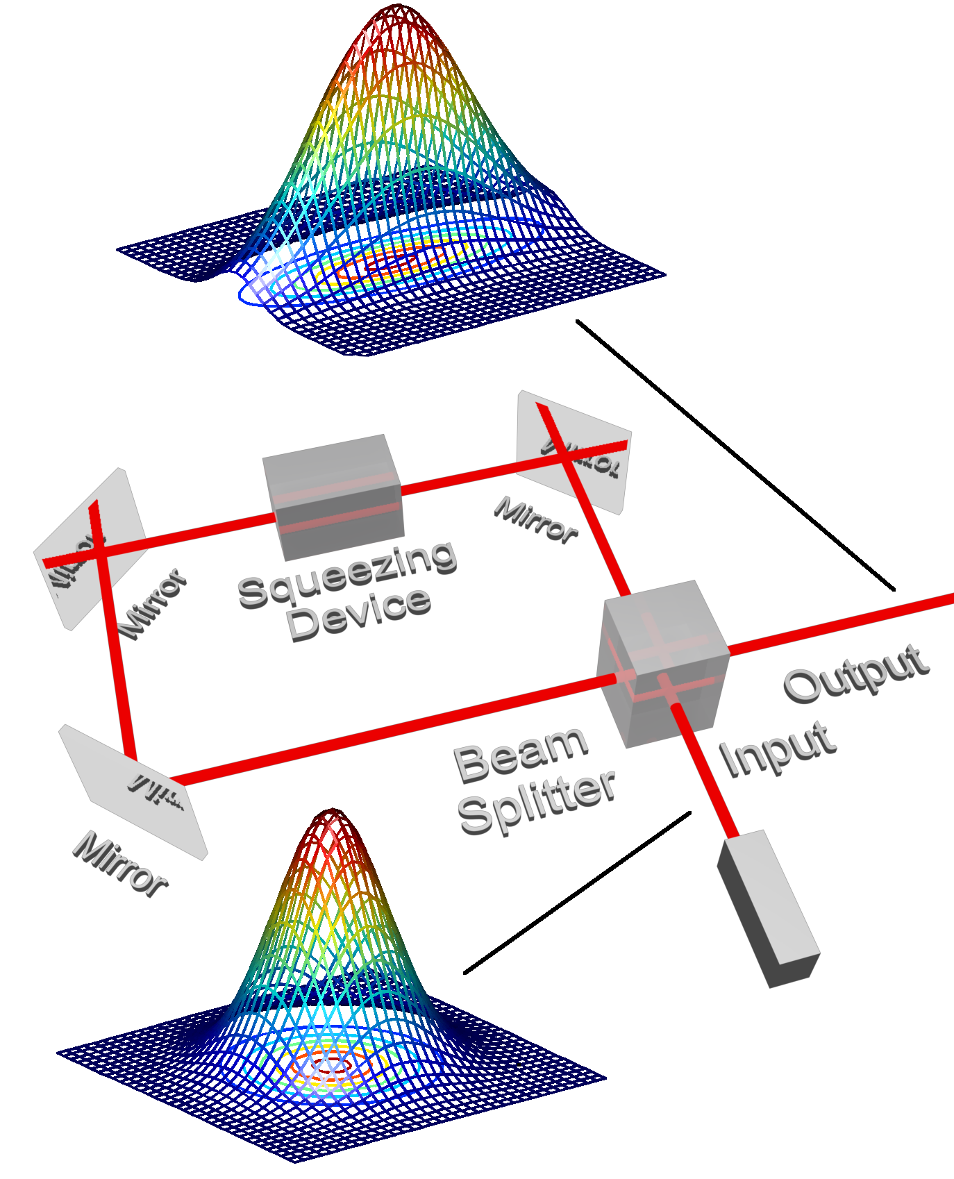
Refer to caption
Figure 1: (Color online) Squeezing Device in a Feedback Loop

The degenerate parametric amplifier (DPA) is a well known non-linear device capable of squeezing input fields [25] -[27]. We follow the treatment of Gardiner [28]. For a single quantum input field coupled to a single cavity mode aa with coupling strength κ\sqrt{\kappa} and Hamiltonian

HDPA=i​ε4​(a∗2−a2),H_{\text{DPA}}=\frac{i\varepsilon}{4}\left(a^{\ast 2}-a^{2}\right), (1)

there is an approximate squeezing parameter given by, [28] section 7.2.9,

rDPA=ln⁡(κ+εκ−ε).r_{\text{DPA}}=\ln\left(\frac{\kappa+\varepsilon}{\kappa-\varepsilon}\right). (2)

Here the amplification is due to the specific choice of the Hamiltonian HDPAH_{\text{DPA}}.

Without feedback, the method of obtaining maximal squeezing for a degenerate parametric amplifier is to try and realize the Hamiltonian for the internal mode with parameter coefficient ε\varepsilon as close to the threshold value (ε=κ)\left(\varepsilon=\kappa\right) as possible, see [28] section 10.2. As originally noted by Yanagisawa and Kimura [24], the value of the effective damping for an in-loop mode, see FIG. 1 will depend on the reflectivity value α\alpha:

κ⁡(α)=1−α1+α​κ.\kappa\left(\alpha\right)=\frac{1-\alpha}{1+\alpha}\kappa. (3)

Our strategy is to use coherent feedback for a fixed degenerate parametric amplifier (below threshold, and therefore internally stable [18])and tune the reflectivity of the beam splitter so as to select the degree of squeezing.

The degenerate parametric amplifier is an idealized device in which one assumes that κ\kappa and ε\varepsilon are large but with fixed ratio. We shall investigate the situation where both these parameters are finite. Also, we introduce additional quantum damping into the model to see the effect of loss.

II Quantum Feedback Networks

A single component consists of a quantum mechanical system, with Hilbert space 𝔥\mathfrak{h} driven by nn quantum input processes bin,i​(i=1,⋯,n)b_{\text{in},i}\left(i=1,\cdots,n\right), [29, 28], satisfying canonical commutation relations of the form [bin,i​(t),bin,j​(t′)]=0[b_{\text{in},i}(t),b_{\text{in},j}(t^{\prime})]=0, [bin,i∗​(t),bin,j∗​(t′)]=0[b_{\text{in},i}^{\ast}(t),b_{\text{in},j}^{\ast}(t^{\prime})]=0 and

[bin,i​(t),bin,j∗​(t′)]=δi​j​δ​(t−t′).[b_{\text{in},i}\left(t\right),b_{\text{in},j}^{\ast}\left(t^{\prime}\right)]=\delta_{ij}\,\delta\left(t-t^{\prime}\right). (4)

A schematic of a component appears in FIG. 2.

The component is characterized by generator G=(S,L,H)G=\left(S,L,H\right) where S=(Si​j)S=\left(S_{ij}\right) is a unitary n×nn\times n matrix whose entries are operators on 𝔥\mathfrak{h} called the scattering coefficient matrix, L=(Li)L=\left(L_{i}\right) is a column vector whose entries are operators on 𝔥\mathfrak{h} called the coupling coefficient vector, and HH is a self-adjoint operator on 𝔥\mathfrak{h} giving the system Hamiltonian. On the joint system-field space we have the unitary evolution process U⁡(t)U\left(t\right) which satisfies the quantum Itō QSDE [30]

dU(t)={∑i,j(Si​j−δi​j)dΛin,i​j(t)+∑iLidBin,i∗(t)−∑i,jLi∗Si​jdBin,j(t)−(12∑iLi∗Li+iH)dt}U(t),dU\left(t\right)=\left\{\sum_{i,j}\left(S_{ij}-\delta_{ij}\right)d\Lambda_{\text{in},ij}\left(t\right)+\sum_{i}L_{i}dB_{\text{in},i}^{\ast}\left(t\right)\right.\\ \left.-\sum_{i,j}L_{i}^{\ast}S_{ij}dB_{\text{in},j}\left(t\right)-(\frac{1}{2}\sum_{i}L_{i}^{\ast}L_{i}+iH)dt\right\}U\left(t\right), (5)

with U⁡(0)=IU(0)=I.

We encounter the integrated fields Bin,i​(t)=∫0tbin,i​(t′)​d​t′B_{\text{in},i}\left(t\right)=\int_{0}^{t}b_{\text{in},i}\left(t^{\prime}\right)dt^{\prime}, Bin,j∗​(t)=Bin,j​(t)∗B_{\text{in},j}^{\ast}\left(t\right)=B_{\text{in},j}\left(t\right)^{\ast} and Λin,i​j​(t)=∫0tbin,i∗​(t′)​bin,j​(t′)​d​t′\Lambda_{\text{in},ij}\left(t\right)=\int_{0}^{t}b_{\text{in},i}^{\ast}\left(t^{\prime}\right)b_{\text{in},j}\left(t^{\prime}\right)dt^{\prime} which satisfy the following quantum Itō table [30]

dBin,i0δi​jdBin,lδi​jdt0dΛin,k​i0δi​jdΛin,k​lδi​jdBin,​k∗0dBin,i∗0000dt0000.\begin{tabular}[]{l|llll}$\times$&$dB_{\text{in},j}$&$d\Lambda_{\text{in},jl}$&$dB_{\text{in},j}^{\ast}$&$dt$\\ \hline\cr$dB_{\text{in},i}$&0&$\delta_{ij}dB_{\text{in},l}$&$\delta_{ij}dt$&0\\ $d\Lambda_{\text{in},ki}$&0&$\delta_{ij}d\Lambda_{\text{in},kl}$&$\delta_{ij}dB_{\text{in,}k}^{\ast}$&0\\ $dB_{\text{in},i}^{\ast}$&0&0&0&0\\ $dt$&0&0&0&0\end{tabular}.
×d​Bin,jd​Λin,j​ld​Bin,j∗d​t
input, b in systemoutput, b out
Figure 2: Input-output component

II.1 Components In Loop

We may consider a feedback arrangement using a beam splitter, as in FIG. 3 below. The beam splitter is a static device which we take to be described by

(boutvin)=T​(binvout),T=(αβμν),\left(\begin{array}[]{c}b_{\text{out}}\\ v_{\text{in}}\end{array}\right)=T\left(\begin{array}[]{c}b_{\text{in}}\\ v_{\text{out}}\end{array}\right),\qquad T=\left(\begin{array}[]{cc}\alpha&\beta\\ \mu&\nu\end{array}\right),

where TT is taken to be a real-valued unitary matrix with determinant σ=α​ν−β​μ=±1\sigma=\alpha\nu-\beta\mu=\pm 1.

Suppose that G10=(S10,L10,H10)G_{1}^{0}=(S_{1}^{0},L_{1}^{0},H_{1}^{0}) is the generator of the (n=1)\left(n=1\right) component before the feedback connections are made. Once the component is in loop, in the limit of instantaneous feedback, we find an effective component with input binb_{\text{in}} and boutb_{\text{out}} as indicated and generator given by G1=(S1,L1,H1)G_{1}=\left(S_{1},L_{1},H_{1}\right) with [13]

S1\displaystyle S_{1} =\displaystyle= α+β⁡((S10)−1−ν)​μ,\displaystyle\alpha+\beta\left(\left(S_{1}^{0}\right)^{-1}-\nu\right)\mu, (6)
L1\displaystyle L_{1} =\displaystyle= β​(1−ν​S10)−1​L10,\displaystyle\beta\left(1-\nu S_{1}^{0}\right)^{-1}L_{1}^{0}, (7)
H1\displaystyle H_{1} =\displaystyle= H10+Im​{(L10)∗​(1−ν​S10)−1​L10}.\displaystyle H_{1}^{0}+\text{Im}\left\{\left(L_{1}^{0}\right)^{\ast}\left(1-\nu S_{1}^{0}\right)^{-1}L_{1}^{0}\right\}. (8)
in-loop device b in b out v in v out
Figure 3: Feedback using a beam-splitter

The example above may be extended to include a loss mechanism describing coupling of the component to the environment, see FIG. 4. Prior to making connections we assume that the component is the four-port system (n=2)\left(n=2\right) with generator given by

S0=(S10001),L0=(L10L20).S_{0}=\left(\begin{array}[]{cc}S_{1}^{0}&0\\ 0&1\end{array}\right),L_{0}=\left(\begin{array}[]{c}L_{1}^{0}\\ L_{2}^{0}\end{array}\right).

After feedback, the effective generator becomes G=(S,L,H)G=\left(S,L,H\right) with

S=(S1001),L=(L1L20),H=H1.S=\left(\begin{array}[]{cc}S_{1}&0\\ 0&1\end{array}\right),L=\left(\begin{array}[]{c}L_{1}\\ L_{2}^{0}\end{array}\right),H=H_{1}.

In the language of [13],[14] the effective generator is the concatenation G=(S1,L1,H1)⊞(1,L20,0)G=\left(S_{1},L_{1},H_{1}\right)\boxplus\left(1,L_{2}^{0},0\right). We have reasoned that since S0S_{0} is diagonal, there is no direct scattering between the inputs to the in loop device, and that concatenation of the effective lossless generator G1G_{1} with the loss mechanism G20G_{2}^{0}. This however can be shown to be correct by utilizing the following construction from [13]: we note that the beam splitter itself can be understood as a static four-port component G′=(T,0,0)G^{\prime}=\left(T,0,0\right) and the set up in FIG. 4 is then naturally identified as a Redheffer star-product arrangement of the two four-port devices, the effective generator for components in a Redheffer formation is given in section 5.3 of [13], and substitution into the expression gives precisely the generator GG.

b in , 1 b out , 1 b out , 2 b in , 2
Figure 4: Feedback with loss

We note that the relations we shall derive below for linear systems can be arrived at by algebraically eliminating the internal fields vinv_{\text{in}} and voutv_{\text{out}}. Whilst this is obviously easier than evoking the mathematical formulation of quantum feedback networks, we should point out that this is not entirely consistent and that the in-loop fields vinv_{\text{in}} and voutv_{\text{out}} are not canonical! Whilst this has been incorrectly interpreted elsewhere as a violation of the Heisenberg uncertainty relations, the reality is that the above description emerges from a regular model in which the commutation relations hold at all times however the finite time delay of the feedback is taken into account [13]. The in-loop fields are eliminated in the instantaneous feedback limit and should then not be thought of as real physical fields. The algebraic arguments presented here, however, reproduce the correct answer.

III Linear State-Based Input-Output Systems

We obtain a linear dynamical model in the case where our system is an assembly of quantum modes aαa_{\alpha} (α=1,⋯,m)\left(\alpha=1,\cdots,m\right) and the components of the generator take the special form Si​jS_{ij} scalars, (using summation convention for repeated indices from now on)

Li\displaystyle L_{i} =\displaystyle= Ci​α−​aα+Ci​α+​aα∗,\displaystyle C_{i\alpha}^{-}a_{\alpha}+C_{i\alpha}^{+}a_{\alpha}^{\ast}, (9)
H\displaystyle H =\displaystyle= ωα​β−​aα∗​aβ+12​ωα​β+​aα∗​aβ∗+12​ωα​β+⁣∗​aα​aβ.\displaystyle\omega_{\alpha\beta}^{-}a_{\alpha}^{\ast}a_{\beta}+\frac{1}{2}\omega_{\alpha\beta}^{+}a_{\alpha}^{\ast}a_{\beta}^{\ast}+\frac{1}{2}\omega_{\alpha\beta}^{+\ast}a_{\alpha}a_{\beta}. (10)

In this case it is possible to apply transform techniques to the dynamical equations. We define the transform fields

b⁡[s]≜∫0∞e−s​t​b​(t)​𝑑t.b\left[s\right]\triangleq\int_{0}^{\infty}e^{-st}b\left(t\right)dt. (11)

Note that

b∗​[s]=(∫0∞e−s∗​t​b​(t)​𝑑t)∗=b​[s∗]∗.b^{\ast}\left[s\right]=(\int_{0}^{\infty}e^{-s^{\ast}t}b\left(t\right)dt)^{\ast}=b\left[s^{\ast}\right]^{\ast}. (12)

Setting bin,i​[s]=∫0∞e−s​t​bin,i​(t)​𝑑tb_{\text{in},i}\left[s\right]=\int_{0}^{\infty}e^{-st}b_{\text{in},i}\left(t\right)dt, etc., we then obtain an input-output relation of the form

bout,i​[s]=Ξi​j−​(s)​bin​[s]+Ξi​j+​(s)​bin,j∗​[s],b_{\text{out},i}\left[s\right]=\Xi_{ij}^{-}\left(s\right)b_{\text{in}}\left[s\right]+\Xi_{ij}^{+}\left(s\right)b_{\text{in},j}^{\ast}\left[s\right], (13)

where Ξi​j∓​(s)\Xi_{ij}^{\mp}\left(s\right) are the transfer functions. (Here we ignore additional terms involving the system modes at initial time. This omission is justified when the model is stable.)

It is convenient to introduce the doubled up notation: for a vector x=(x1,⋯,xN)⊤x=\left(x_{1},\cdots,x_{N}\right)^{\top}, we write x˘=(x1,⋯xN,x1∗,⋯,xN∗)⊤\breve{x}=\left(x_{1},\cdots x_{N},x_{1}^{\ast},\cdots,x_{N}^{\ast}\right)^{\top} where ⊤\top is transposition, for N×MN\times M matrices A,BA,B we write Δ⁡(A,B)=[ABB♯A♯]\Delta\left(A,B\right)=\left[\begin{array}[]{cc}A&B\\ B^{\sharp}&A^{\sharp}\end{array}\right] where ♯\sharp is entry-wise conjugation, [Ai​j]♯=[Ai​j∗]\left[A_{ij}\right]^{\sharp}=\left[A_{ij}^{\ast}\right]. We also set Δ​(A,B)♭=Δ⁡(A†,−B⊤)\Delta\left(A,B\right)^{\flat}=\Delta\left(A^{{\dagger}},-B^{\top}\right) where † is the usual hermitian conjugation. We say that a matrix S~=Δ⁡(S−,S+)\tilde{S}=\Delta\left(S_{-},S_{+}\right) is Bogoliubov, or symplectic, if it is invertible with

S~♭=S~−1.\tilde{S}^{\flat}=\tilde{S}^{-1}.

The transfer relation can be written as

b˘out​[s]=Ξ~​(s)​b˘in​[s]\breve{b}_{\text{out}}\left[s\right]=\tilde{\Xi}\left(s\right)\breve{b}_{\text{in}}\left[s\right]

with transfer matrix function

Ξ~​(s)=[Ξ−​(s)Ξ+​(s)Ξ+​(s)♯Ξ−​(s)♯].\tilde{\Xi}\left(s\right)=\left[\begin{array}[]{cc}\Xi^{-}\left(s\right)&\Xi^{+}\left(s\right)\\ \Xi^{+}\left(s\right)^{\sharp}&\Xi^{-}\left(s\right)^{\sharp}\end{array}\right].

Explicitly

Ξ~​(s)=[I2​n−C~​(s​I2​m−A~)−1​C~♭]​S~\tilde{\Xi}\left(s\right)=\left[I_{2n}-\tilde{C}\left(sI_{2m}-\tilde{A}\right)^{-1}\tilde{C}^{\flat}\right]\tilde{S} (14)

where S~=Δ⁡(S,0)\tilde{S}=\Delta\left(S,0\right), C~=Δ⁡(C−,C+)\tilde{C}=\Delta\left(C_{-},C_{+}\right) where C∓=[Ci​α∓]C_{\mp}=\left[C_{i\alpha}^{\mp}\right], A~=−12​C~♭​C~−i​Ω~\tilde{A}=-\frac{1}{2}\tilde{C}^{\flat}\tilde{C}-i\tilde{\Omega} where Ω~=Δ⁡(Ω−,Ω+)\tilde{\Omega}=\Delta\left(\Omega_{-},\Omega_{+}\right) with Ω∓=[ωα​β∓]\Omega_{\mp}=\left[\omega_{\alpha\beta}^{\mp}\right].

III.1 Analysis of the Spectrum

In addition to the fields b⁡[s]b\left[s\right] in (11)\left(\ref{TB}\right) we also define past-field transforms

c⁡[s]≜∫−∞0e−s​t​b​(t)​𝑑tc\left[s\right]\triangleq\int_{-\infty}^{0}e^{-st}b\left(t\right)dt (15)

We remark that for input process as arguments, the fields b⁡[s]b\left[s\right] and b∗​[s]b^{\ast}\left[s\right] commute with the fields c⁡[s′]c\left[s^{\prime}\right] and c∗​[s′]c^{\ast}\left[s^{\prime}\right] for all parameters s,s′s,s^{\prime} since they involve integrals over future and past input fields respectively.

The Fourier transform of a field bb is then defined to be

b^​(ω)\displaystyle\hat{b}\left(\omega\right) =\displaystyle= 12​π​∫−∞∞ei​ω​t​b​(t)​𝑑t\displaystyle\frac{1}{\sqrt{2\pi}}\int_{-\infty}^{\infty}e^{i\omega t}b\left(t\right)dt
≡\displaystyle\equiv 12​π​b​[0+−i​ω]+12​π​c​[0−−i​ω].\displaystyle\frac{1}{\sqrt{2\pi}}b\left[0^{+}-i\omega\right]+\frac{1}{\sqrt{2\pi}}c\left[0^{-}-i\omega\right].

The canonical commutation relations (4) then imply that [b^in,​i​(ω),b^in,​j​(ω′)∗]=δi​j​δ​(ω−ω′)\left[\hat{b}_{\text{in,}i}\left(\omega\right),\hat{b}_{\text{in,}j}\left(\omega^{\prime}\right)^{\ast}\right]=\delta_{ij}\delta\left(\omega-\omega^{\prime}\right). In the vacuum state we have

⟨bin,​i​[0+−i​ω]​bin,​j∗​[0+−i​ω′]⟩\displaystyle\langle b_{\text{in,}i}\left[0^{+}-i\omega\right]b_{\text{in,}j}^{\ast}\left[0^{+}-i\omega^{\prime}\right]\rangle =\displaystyle= δi​j​ζ+​(ω+ω′),\displaystyle\delta_{ij}\zeta_{+}\left(\omega+\omega^{\prime}\right),
⟨cin,​i​[0−−i​ω]​cin,​j∗​[0−−i​ω′]⟩\displaystyle\langle c_{\text{in,}i}\left[0^{-}-i\omega\right]c_{\text{in,}j}^{\ast}\left[0^{-}-i\omega^{\prime}\right]\rangle =\displaystyle= δi​j​ζ−​(ω+ω′),\displaystyle\delta_{ij}\zeta_{-}\left(\omega+\omega^{\prime}\right),

where the Heitler functions are

ζ+​(ω)=∫0∞ei​ω​t​𝑑t,ζ−​(ω)=∫−∞0ei​ω​t​𝑑t,\zeta_{+}\left(\omega\right)=\int_{0}^{\infty}e^{i\omega t}dt,\,\,\zeta_{-}\left(\omega\right)=\int_{-\infty}^{0}e^{i\omega t}dt,

or

ζ±​(ω)=π​δ​(ω)±i​P​V​1ω.\zeta_{\pm}\left(\omega\right)=\pi\delta\left(\omega\right)\pm iPV\frac{1}{\omega}.

In practice we shall only encounter the combination ζ++ζ−=2​π​δ\zeta_{+}+\zeta_{-}=2\pi\delta when calculating physical correlations, and not encounter the principle value contribution. In particular,

⟨b^in,​i​(ω)​b^in,​j∗​(ω′)⟩=δi​j​δ​(ω−ω′),\langle\hat{b}_{\text{in,}i}\left(\omega\right)\hat{b}_{\text{in,}j}^{\ast}\left(\omega^{\prime}\right)\rangle=\delta_{ij}\delta\left(\omega-\omega^{\prime}\right), (16)

as we have the sum of 12​π​⟨bin,​i​[0+−i​ω]​bin,​j∗​[0++i​ω′]⟩\frac{1}{2\pi}\langle b_{\text{in,}i}\left[0^{+}-i\omega\right]b_{\text{in,}j}^{\ast}\left[0^{+}+i\omega^{\prime}\right]\rangle and 12​π​⟨cin,​i​[0−−i​ω]​cin,​j∗​[0−+i​ω′]⟩\frac{1}{2\pi}\langle c_{\text{in,}i}\left[0^{-}-i\omega\right]c_{\text{in,}j}^{\ast}\left[0^{-}+i\omega^{\prime}\right]\rangle. Likewise

⟨b^in,​i∗​(ω)​b^in,​j​(ω′)⟩=⟨b^in,​i​(ω)​b^in,​j​(ω′)⟩\displaystyle\langle\hat{b}_{\text{in,}i}^{\ast}\left(\omega\right)\hat{b}_{\text{in,}j}\left(\omega^{\prime}\right)\rangle=\langle\hat{b}_{\text{in,}i}\left(\omega\right)\hat{b}_{\text{in,}j}\left(\omega^{\prime}\right)\rangle
=⟨b^in,​i∗​(ω)​b^in,​j∗​(ω′)⟩=0.\displaystyle=\langle\hat{b}_{\text{in,}i}^{\ast}\left(\omega\right)\hat{b}_{\text{in,}j}^{\ast}\left(\omega^{\prime}\right)\rangle=0.

Ignoring the contribution from the initial value of the internal mode, the input-output relations for the past fields takes a similar form to (13) namely

cout,i​[s]=Ξi​j−​(s)​cin,j​[s]+Ξi​j+​(s)​cin,j∗​[s],c_{\text{out},i}\left[s\right]=\Xi_{ij}^{-}\left(s\right)c_{\text{in},j}\left[s\right]+\Xi_{ij}^{+}\left(s\right)c_{\text{in},j}^{\ast}[s],

the only essential difference in the calculation being the sign change. Let us introduce the matrices

𝒮i​j−​(ω)=Ξi​j−​(−i​ω),𝒮i​j+​(ω)=Ξi​j+​(−i​ω)\mathcal{S}_{ij}^{-}\left(\omega\right)=\Xi_{ij}^{-}\left(-i\omega\right),\quad\mathcal{S}_{ij}^{+}\left(\omega\right)=\Xi_{ij}^{+}\left(-i\omega\right) (17)

then

b^out,i​(ω)=𝒮i​j−​(ω)​b^in,j​(ω)+𝒮i​j+​(ω)​b^in,j​(−ω)∗.\hat{b}_{\text{out},i}\left(\omega\right)=\mathcal{S}_{ij}^{-}\left(\omega\right)\hat{b}_{\text{in},j}\left(\omega\right)+\mathcal{S}_{ij}^{+}\left(\omega\right)\hat{b}_{\text{in},j}\left(-\omega\right)^{\ast}. (18)

We may therefore determine the correlation functions from the transfer functions given that the input is in the vacuum state:

⟨b^out,i∗​(ω)​b^out,j​(ω′)⟩\displaystyle\left\langle\hat{b}_{\text{out},i}^{\ast}\left(\omega\right)\hat{b}_{\text{out},j}\left(\omega^{\prime}\right)\right\rangle =\displaystyle= 𝒩i​j​(ω)​δ​(ω−ω′),\displaystyle\mathcal{N}_{ij}\left(\omega\right)\,\delta\left(\omega-\omega^{\prime}\right),
⟨b^out,i​(ω)​b^out,j​(ω′)⟩\displaystyle\left\langle\hat{b}_{\text{out},i}\left(\omega\right)\hat{b}_{\text{out},j}\left(\omega^{\prime}\right)\right\rangle =\displaystyle= ℳi​j​(ω)​δ​(ω+ω′),\displaystyle\mathcal{M}_{ij}\left(\omega\right)\,\delta\left(\omega+\omega^{\prime}\right), (19)

where

𝒩i​j​(ω)=𝒮i​k+​(ω)∗​𝒮j​k+​(ω),ℳi​j​(ω)=𝒮i​k−​(ω)​𝒮j​k+​(−ω).\mathcal{N}_{ij}\left(\omega\right)=\mathcal{S}_{ik}^{+}\left(\omega\right)^{\ast}\mathcal{S}_{jk}^{+}\left(\omega\right),\;\mathcal{M}_{ij}\left(\omega\right)=\mathcal{S}_{ik}^{-}\left(\omega\right)\mathcal{S}_{jk}^{+}\left(-\omega\right). (20)

We note the straightforward identities

𝒩i​j​(ω)∗=𝒩j​i​(ω),ℳi​j​(ω)∗=ℳj​i​(−ω).\mathcal{N}_{ij}\left(\omega\right)^{\ast}=\mathcal{N}_{ji}\left(\omega\right),\quad\mathcal{M}_{ij}\left(\omega\right)^{\ast}=\mathcal{M}_{ji}\left(-\omega\right).

We remark that

Ξ~​(−i​ω)≡Δ⁡(𝒮−​(ω),𝒮+​(ω))\tilde{\Xi}\left(-i\omega\right)\equiv\Delta\left(\mathcal{S}_{-}\left(\omega\right),\mathcal{S}_{+}\left(\omega\right)\right)

and that this defines a Bogoliubov matrix for each real ω\omega where it is well-defined, see [18] subsection V.C. In particular, this ensures that the transformation from inputs to outputs is canonical, and the Fourier transform of the outputs satisfy a similar relation to (16)\left(\ref{bfin}\right). We see directly from (14)\left(\ref{TFform}\right) that lim|ω|→∞Ξ~​(−i​ω)=Δ⁡(S,0)\lim_{|\omega|\rightarrow\infty}\tilde{\Xi}\left(-i\omega\right)=\Delta(S,0), or

lim|ω|→∞𝒮−​(ω)=S,lim|ω|→∞𝒮+​(ω)=0.\lim_{|\omega|\rightarrow\infty}\mathcal{S}_{-}\left(\omega\right)=S,\;\lim_{|\omega|\rightarrow\infty}\mathcal{S}_{+}\left(\omega\right)=0. (21)

Definition: We say that a component is capable of spectral squeezing if the matrix ℳ⁡(ω)\mathcal{M}\left(\omega\right) is non zero for certain frequencies ω\omega. In particular, given a vacuum input, we say that the iith mode is spectrally squeezed if ℳi​i​(ω)≠0\mathcal{M}_{ii}\left(\omega\right)\neq 0 for some ω\omega.

In the single input situation, the 𝒮∓​(ω)\mathcal{S}_{\mp}\left(\omega\right) are complex-valued functions satisfying |𝒮−​(ω)|2−|𝒮+​(ω)|2=1|\mathcal{S}_{-}\left(\omega\right)|^{2}-|\mathcal{S}_{+}\left(\omega\right)|^{2}=1. We then define the spectral squeezing function r⁡(ω)r\left(\omega\right) by |𝒮−​(ω)|=cosh⁡r⁡(ω)|\mathcal{S}_{-}\left(\omega\right)|=\cosh r\left(\omega\right), that is

r⁡(ω)\displaystyle r\left(\omega\right) =\displaystyle= 12​ln⁡|𝒮−​(ω)|+|𝒮+​(ω)||𝒮−​(ω)|−|𝒮+​(ω)|\displaystyle\frac{1}{2}\ln\frac{|\mathcal{S}_{-}\left(\omega\right)|+|\mathcal{S}_{+}\left(\omega\right)|}{|\mathcal{S}_{-}\left(\omega\right)|-|\mathcal{S}_{+}\left(\omega\right)|} (22)
≡\displaystyle\equiv ln⁡{|𝒮−​(ω)|+|𝒮+​(ω)|}.\displaystyle\ln\left\{|\mathcal{S}_{-}\left(\omega\right)|+|\mathcal{S}_{+}\left(\omega\right)|\right\}.

III.2 Power Spectrum Density

We define output quadratures by

qout,i​(t,θ)=ei​θ​bout,i​(t)+e−i​θ​bout,i​(t)∗,q_{\text{out},i}\left(t,\theta\right)=e^{i\theta}b_{\text{out},i}\left(t\right)+e^{-i\theta}b_{\text{out},i}\left(t\right)^{\ast}, (23)

for fixed phases θ∈[0,2​π)\theta\in[0,2\pi). The integrated processes Qout,i​(t,θ)=∫0tqout,i​(t′,θ)​d​t′Q_{\text{out},i}\left(t,\theta\right)=\int_{0}^{t}q_{\text{out},i}\left(t^{\prime},\theta\right)dt^{\prime} are self-commuting for fixed θ\theta and different times tt and indices ii, and correspond to classical diffusion processes with Itō differentials satisfying

d​Qout,i​(t,θ)​d​Qout,j​(t,θ)=δi​j​d​t.dQ_{\text{out},i}\left(t,\theta\right)\,dQ_{\text{out},j}\left(t,\theta\right)=\delta_{ij}dt. (24)

Following Barchielli and Gregoratti [32], we set

𝒫i​j​(ω,θ,T)\displaystyle\mathcal{P}_{ij}(\omega,\theta,T) =\displaystyle= 1T⟨∫0Tei​ω​t1qout,i(t1,θ)dt1\displaystyle\frac{1}{T}\langle\int_{0}^{T}e^{i\omega t_{1}}q_{\text{out},i}\left(t_{1},\theta\right)dt_{1}
×∫0Te−i​ω​t2qout,i(t2,θ)dt2⟩,\displaystyle\times\int_{0}^{T}e^{-i\omega t_{2}}q_{\text{out},i}\left(t_{2},\theta\right)dt_{2}\rangle,
𝒫i​jel​(ω,θ,T)\displaystyle\mathcal{P}_{ij}^{\text{el}}(\omega,\theta,T) =\displaystyle= 1T​⟨∫0Tei​ω​t1​qout,i​(t1,θ)​d​t1⟩\displaystyle\frac{1}{T}\langle\int_{0}^{T}e^{i\omega t_{1}}q_{\text{out},i}\left(t_{1},\theta\right)dt_{1}\rangle
×⟨∫0Te−i​ω​t2​qout,i​(t2,θ)​d​t2⟩,\displaystyle\times\langle\int_{0}^{T}e^{-i\omega t_{2}}q_{\text{out},i}\left(t_{2},\theta\right)dt_{2}\rangle,
𝒫i​jinel​(ω,θ,T)\displaystyle\mathcal{P}_{ij}^{\text{inel}}(\omega,\theta,T) =\displaystyle= 𝒫i​j​(ω,θ,T)−𝒫i​jel​(ω,θ,T),\displaystyle\mathcal{P}_{ij}(\omega,\theta,T)-\mathcal{P}_{ij}^{\text{el}}(\omega,\theta,T),

and define the power spectral density matrix to be

𝒫i​j​(ω,θ)=limT→∞𝒫i​j​(ω,θ,T),\mathcal{P}_{ij}(\omega,\theta)=\lim_{T\rightarrow\infty}\mathcal{P}_{ij}(\omega,\theta,T), (25)

whenever the limits exist, along with the elastic and inelastic components 𝒫i​jel​(ω,θ)=limT→∞𝒫i​jel​(ω,θ,T)\mathcal{P}_{ij}^{\text{el}}(\omega,\theta)=\lim_{T\rightarrow\infty}\mathcal{P}_{ij}^{\text{el}}(\omega,\theta,T), 𝒫i​jinel​(ω,θ)=limT→∞𝒫i​jinel​(ω,θ,T)\mathcal{P}_{ij}^{\text{inel}}(\omega,\theta)=\lim_{T\rightarrow\infty}\mathcal{P}_{ij}^{\text{inel}}(\omega,\theta,T) respectively.

The Itō rule (24)\left(\ref{dQ2}\right) implies that

𝒫i​jinel​(ω,θ)=δi​j,\mathcal{P}_{ij}^{\text{inel}}(\omega,\theta)=\delta_{ij}, (26)

and this may be interpreted by saying that the squeezing in the dynamic model comes entirely from the elastic component, and that there is no inelastic squeezing.

The Fourier transform is then q^out,i​(ω,θ)=ei​θ​b^out,i​(ω)+e−i​θ​b^out,i​(−ω)∗\hat{q}_{\text{out},i}\left(\omega,\theta\right)=e^{i\theta}\hat{b}_{\text{out},i}\left(\omega\right)+e^{-i\theta}\hat{b}_{\text{out},i}\left(-\omega\right)^{\ast} and it is readily verified that, for vacuum input,

⟨q^out,i​(ω,θ)​q^out,j​(ω′,θ)⟩=𝒫i​j​(ω,θ)​δ​(ω+ω′)\langle\hat{q}_{\text{out},i}\left(\omega,\theta\right)\hat{q}_{\text{out},j}\left(\omega^{\prime},\theta\right)\rangle=\mathcal{P}_{ij}\left(\omega,\theta\right)\delta\left(\omega+\omega^{\prime}\right) (27)

where we obtain the explicit expression

𝒫i​j​(ω,θ)\displaystyle\mathcal{P}_{ij}\left(\omega,\theta\right) =\displaystyle= δi​j+𝒩i​j​(−ω)+𝒩j​i​(ω)\displaystyle\delta_{ij}+\mathcal{N}_{ij}\left(-\omega\right)+\mathcal{N}_{ji}\left(\omega\right) (28)
+\displaystyle+ e2​i​θ​ℳj​i​(ω)+e−2​i​θ​ℳi​j​(−ω)∗.\displaystyle e^{2i\theta}\mathcal{M}_{ji}\left(\omega\right)+e^{-2i\theta}\mathcal{M}_{ij}\left(-\omega\right)^{\ast}.

III.3 Idealized Static Squeezing Components

A static squeezing device is an idealized static component with input-output relation of the form (either in the time or transform domain)

bout,i=Si​j−​bin,j+Si​j+​bin,j∗b_{\text{out},i}=S_{ij}^{-}b_{\text{in},j}+S_{ij}^{+}b_{\text{in},j}^{\ast} (29)

where S∓=[Si​j∓]∈ℂn×nS_{\mp}=\left[S_{ij}^{\mp}\right]\in\mathbb{C}^{n\times n} are constant coefficients such that S~=Δ⁡(S−,S+)\tilde{S}=\Delta\left(S_{-},S_{+}\right) is a Bogoliubov matrix. The outputs are then a symplectic transformation of the inputs and therefore satisfy the canonical commutation relations.

In practice, such a device is realized approximately by a dynamical component, in a limiting regime. Specifically, we would require in the Fourier domain that the coefficients 𝒮i​j∓​(ω)\mathcal{S}_{ij}^{\mp}\left(\omega\right) in (18)\left(\ref{bfio}\right) are approximately constant over a wide range of frequencies.

Definition: We say that a sequence of models converges pointwise in transfer function if we have limk→∞Ξ~k​(ω)=Ξ~​(ω)\lim_{k\rightarrow\infty}\tilde{\Xi}_{k}\left(\omega\right)=\tilde{\Xi}\left(\omega\right).

If the limit is a Bogoliubov matrix S~=Δ⁡(S−,S+)\tilde{S}=\Delta\left(S_{-},S_{+}\right) independent of ss, then we obtain a static device. In this case, if S+=0S_{+}=0 then S−S_{-} is unitary and the limit corresponds to a beam splitter with S=S−S=S_{-}. The situation S+≠0S_{+}\neq 0 can however arise as such limits, the DPA is an example, and we refer to such idealized components as static squeezing devices. This notion of convergence is weak since there is no quantum stochastic limit model for which we could obtain S+≠0S_{+}\neq 0, specifically we would violate the requirement (21)\left(\ref{S asymptotic}\right) common to all dynamical models considered up to this point.

For the case of a single input (OPENn=1)n=1), the S∓S_{\mp} are scalars with the constraint |S−|2−|S+|2=1,|S_{-}|^{2}-|S_{+}|^{2}=1,which ensures preservation of the canonical commutation relations. The parameter r=cosh⁡|S−|r=\cosh|S_{-}| is referred to as the squeezing parameter. We then have |S−|=cosh⁡r|S_{-}|=\cosh r, |S+|=sinh⁡r|S_{+}|=\sinh r, and we find that the extremal squeezing ratios of quadratures by the device are e±re^{\pm r}.

We should remark that the canonical transformation in equation (29) is a Bogoliubov transformation for a quantum field. There is a strict condition on when Bogoliubov transformations are unitarily implemented for infinite dimensional systems (Shale’s Theorem, [31]) which are not met in this particular case.

IV The Degenerate Parametric Amplifier

We now treat the specific example of a degenerate parametric amplifier.

IV.1 Lossy DPA, Open Loop

We consider n=2n=2 input field processes driving a single (m=1)\left(m=1\right) mode with

S=[1001],L=[κ​aγ​a]S=\left[\begin{array}[]{cc}1&0\\ 0&1\end{array}\right],L=\left[\begin{array}[]{c}\sqrt{\kappa}a\\ \sqrt{\gamma}a\end{array}\right]

and H=HDPAH=H_{\text{DPA}} as in (1)\left(\ref{H_DPA}\right). Here C−=[κγ]C_{-}=\left[\begin{array}[]{c}\sqrt{\kappa}\\ \sqrt{\gamma}\end{array}\right], C+=0C_{+}=0, Ω−=0\Omega_{-}=0 and Ω+=ε2\Omega_{+}=\frac{\varepsilon}{2}. Therefore A~=−12​[κ+γ−ε−εκ+γ]\tilde{A}=-\frac{1}{2}\left[\begin{array}[]{cc}\kappa+\gamma&-\varepsilon\\ -\varepsilon&\kappa+\gamma\end{array}\right], and we see that the system is Hurwitz stable (that is, A~\tilde{A} has all eigenvalues in the negative half plane) if

κ+γ>ε.\kappa+\gamma>\varepsilon. (30)

We obtain the following expressions for Ξ∓​(s)=[Ξi​j∓​(s)]\Xi_{\mp}\left(s\right)=\left[\Xi_{ij}^{\mp}\left(s\right)\right]:

Ξ−​(s)\displaystyle\Xi_{-}\left(s\right) =\displaystyle=
1P⁡(s)​[s2+γ​s+γ2−κ2−ε24−κ​γ​(s+κ+γ2)−κ​γ​(s+κ+γ2)s2+κ​s+κ2−γ2−ε24],\displaystyle\frac{1}{P\left(s\right)}\left[\begin{array}[]{cc}s^{2}+\gamma s+\frac{\gamma^{2}-\kappa^{2}-\varepsilon^{2}}{4}&-\sqrt{\kappa\gamma}\left(s+\frac{\kappa+\gamma}{2}\right)\\ -\sqrt{\kappa\gamma}\left(s+\frac{\kappa+\gamma}{2}\right)&s^{2}+\kappa s+\frac{\kappa^{2}-\gamma^{2}-\varepsilon^{2}}{4}\end{array}\right],
Ξ+​(s)\displaystyle\Xi_{+}\left(s\right) =−ε2​P​(s)​[κκ​γκ​γγ],\displaystyle=-\frac{\varepsilon}{2P\left(s\right)}\left[\begin{array}[]{cc}\kappa&\sqrt{\kappa\gamma}\\ \sqrt{\kappa\gamma}&\gamma\end{array}\right],

where

P⁡(s)=(s+κ+γ2+ε2)​(s+κ+γ2−ε2).P\left(s\right)=\left(s+\frac{\kappa+\gamma}{2}+\frac{\varepsilon}{2}\right)\left(s+\frac{\kappa+\gamma}{2}-\frac{\varepsilon}{2}\right). (35)

This gives the transfer function for the component in FIG.3 prior to feedback connection.

IV.2 Lossy DPA, Closed Loop

Let us take for definiteness the beam splitter matrix to be

T⁡(α)=[αββ−α],T\left(\alpha\right)=\left[\begin{array}[]{cc}\alpha&\beta\\ \beta&-\alpha\end{array}\right], (36)

where 0<α<10<\alpha<1 and β=1−α2\beta=\sqrt{1-\alpha^{2}}. Following our discussions in the previous section, the actual situation modeled in FIG.3 is then given by replacing L1L_{1} by

L1​(α)=β⁡(1−ν)​L1≡κ⁡(α)​aL_{1}\left(\alpha\right)=\beta\left(1-\nu\right)L_{1}\equiv\sqrt{\kappa\left(\alpha\right)}a (37)

where κ⁡(α)=1−α1+α​κ\kappa\left(\alpha\right)=\frac{1-\alpha}{1+\alpha}\kappa in accordance with (3)\left(\ref{kappa_eff}\right). The transfer function is therefore of the same form as derived in (IV.1,35)\left(\ref{TF},\ref{P}\right) but with κ\kappa now replaced by κ⁡(α)\kappa\left(\alpha\right).

IV.3 Spectrum of the DPA Output

We are interested in the input-output relation between bin,1b_{\text{in,1}} and bout,1b_{\text{out,1}}. Here, displaying the dependence on α\alpha, we compute

𝒩11​(ω,α)=ε2​κ​(α)​(κ⁡(α)+γ)4​D​(ω,α),ℳ11​(ω,α)=ε​κ​(α)2​D​(ω,α)​[ω2+(κ⁡(α)+γ2)2+(ε2)2]\mathcal{N}_{11}\left(\omega,\alpha\right)=\frac{\varepsilon^{2}\kappa(\alpha)\left(\kappa(\alpha)+\gamma\right)}{4D(\omega,\alpha)},\quad\mathcal{M}_{11}\left(\omega,\alpha\right)=\frac{\varepsilon\kappa(\alpha)}{2D(\omega,\alpha)}\left[\omega^{2}+\left(\frac{\kappa(\alpha)+\gamma}{2}\right)^{2}+\left(\frac{\varepsilon}{2}\right)^{2}\right] (38)

with

D⁡(ω,α)=|P⁡(−i​ω,α)|2=[ω2+(κ⁡(α)+γ+ε2)2]​[ω2+(κ⁡(α)+γ−ε2)2].D(\omega,\alpha)=|P\left(-i\omega,\alpha\right)|^{2}=\left[\omega^{2}+\left(\frac{\kappa(\alpha)+\gamma+\varepsilon}{2}\right)^{2}\right]\left[\omega^{2}+\left(\frac{\kappa(\alpha)+\gamma-\varepsilon}{2}\right)^{2}\right]. (39)

Note that in the lossless situation γ=0\gamma=0, we have |𝒮11−​(ω,α)|2−|𝒮11+​(ω,α)|2=1|\mathcal{S}_{11}^{-}\left(\omega,\alpha\right)|^{2}-|\mathcal{S}_{11}^{+}\left(\omega,\alpha\right)|^{2}=1 and therefore the identity |ℳ11​(ω,α)|2=(𝒩11​(ω,α)+1)​𝒩11​(ω,α)|\mathcal{M}_{11}(\omega,\alpha)|^{2}=(\mathcal{N}_{11}(\omega,\alpha)+1)\mathcal{N}_{11}(\omega,\alpha). In particular, we compute that the spectral squeezing function is

r⁡(ω,α)=12​ln⁡ω2+(κ⁡(α)+ε2)2ω2+(κ⁡(α)−ε2)2.r\left(\omega,\alpha\right)=\frac{1}{2}\ln\frac{\omega^{2}+\left(\frac{\kappa(\alpha)+\varepsilon}{2}\right)^{2}}{\omega^{2}+\left(\frac{\kappa(\alpha)-\varepsilon}{2}\right)^{2}}. (40)

In this case we find that we find that the power spectral density 𝒫11​(ω,θ)\mathcal{P}_{11}\left(\omega,\theta\right) is

[ω2+κ​(α)2+ε24]2+κ​(α)2​ε24+ε​κ​(α)​[ω2+κ​(α)2+ε24]​cos⁡2​θD⁡(ω,α),\frac{\left[\omega^{2}+\frac{\kappa(\alpha)^{2}+\varepsilon^{2}}{4}\right]^{2}+\frac{\kappa(\alpha)^{2}\varepsilon^{2}}{4}+\varepsilon\kappa(\alpha)\left[\omega^{2}+\frac{\kappa(\alpha)^{2}+\varepsilon^{2}}{4}\right]\cos 2\theta}{D\left(\omega,\alpha\right)},

with the maximum squeezing at θ=0\theta=0, 𝒫11​(ω,0)=e2​r​(α,ω)\mathcal{P}_{11}\left(\omega,0\right)=e^{2r(\alpha,\omega)} and minimum squeezing at θ=π2\theta=\frac{\pi}{2}, 𝒫11​(ω,π2)=e−2​r​(α,ω)\mathcal{P}_{11}\left(\omega,\frac{\pi}{2}\right)=e^{-2r(\alpha,\omega)}.

IV.4 The Static Limit of the DPA

We consider a sequence of DPA models described by the parameters (κk,εk,γk)k≥1\left(\kappa_{k},\varepsilon_{k},\gamma_{k}\right)_{k\geq 1} with

κk=k​κ,εk=k​ε,γk=k​γ,\kappa_{k}=k\kappa,\;\varepsilon_{k}=k\varepsilon,\;\gamma_{k}=k\gamma,

and consider the singular limit k→∞k\rightarrow\infty. We note that Ξ∓(k)​(s)≡Ξ∓​(s/k)\Xi_{\mp}^{\left(k\right)}\left(s\right)\equiv\Xi_{\mp}\left(s/k\right) so the limit is equivalent to the low frequency limit. The limit transfer functions are independent of the transform variable ss:

S−\displaystyle S_{-} =\displaystyle= limk→∞Ξ−(k)​(s)\displaystyle\lim_{k\rightarrow\infty}\Xi_{-}^{\left(k\right)}\left(s\right)
=\displaystyle= 1(κ+γ)2−ε2​[γ2−κ2−ε2−2​κ​γ​(κ+γ)−2​κ​γ​(κ+γ)κ2−γ2−ε2],\displaystyle\frac{1}{\left(\kappa+\gamma\right)^{2}-\varepsilon^{2}}\left[\begin{array}[]{cc}\gamma^{2}-\kappa^{2}-\varepsilon^{2}&-2\sqrt{\kappa\gamma}\left(\kappa+\gamma\right)\\ -2\sqrt{\kappa\gamma}\left(\kappa+\gamma\right)&\kappa^{2}-\gamma^{2}-\varepsilon^{2}\end{array}\right],
S+\displaystyle S_{+} =\displaystyle= limk→∞Ξ+(k)​(s)=−2​ε(κ+γ)2−ε2​[κκ​γκ​γγ].\displaystyle\lim_{k\rightarrow\infty}\Xi_{+}^{\left(k\right)}\left(s\right)=\frac{-2\varepsilon}{\left(\kappa+\gamma\right)^{2}-\varepsilon^{2}}\left[\begin{array}[]{cc}\kappa&\sqrt{\kappa\gamma}\\ \sqrt{\kappa\gamma}&\gamma\end{array}\right].

In particular, S~=Δ⁡(S−,S+)\tilde{S}=\Delta\left(S_{-},S_{+}\right) is a Bogoliubov matrix. The squeezing parameter for the limit Bogoliubov transformation is then

r=ln⁡(κ+εκ−ε),r=\ln\left(\frac{\kappa+\varepsilon}{\kappa-\varepsilon}\right),

or equivalently r⁡(0)r\left(0\right) in (22)\left(\ref{r_omega}\right). This is of course the equation (2)\left(\ref{r_open_loop}\right).

The central issue here is that the asymptotic limit |ω|→∞|\omega|\rightarrow\infty and the transfer function convergence limit k→∞k\rightarrow\infty do not commute: denoting the spectral squeezing functions for the sequence of models as r(k)​(ω)r^{\left(k\right)}\left(\omega\right) we have limk→∞r(k)​(ω)=r\lim_{k\rightarrow\infty}r^{\left(k\right)}\left(\omega\right)=r for all ω\omega, while lim|ω|→∞r(k)​(ω)=0\lim_{|\omega|\rightarrow\infty}r^{\left(k\right)}\left(\omega\right)=0 for all kk.

We likewise find that the inelastic contribution to the power spectrum of the limit output quadratures is given by (θ=0)\left(\theta=0\right)

𝒫inel(θ=0)=(κ+γ+ε)2[(κ+γ)2−ε2]2×\mathcal{P}^{\text{inel}}\left(\theta=0\right)=\frac{\left(\kappa+\gamma+\varepsilon\right)^{2}}{\left[\left(\kappa+\gamma\right)^{2}-\varepsilon^{2}\right]^{2}}\times
[(κ+γ)2+ε2−2​ε​(γ−κ)4​κ​γ​ε4​κ​γ​ε(κ+γ)2+ε2+2​ε​(γ−κ)]\left[\begin{array}[]{cc}(\kappa+\gamma)^{2}+\varepsilon^{2}-2\varepsilon(\gamma-\kappa)&4\sqrt{\kappa\gamma}\varepsilon\\ 4\sqrt{\kappa\gamma}\varepsilon&(\kappa+\gamma)^{2}+\varepsilon^{2}+2\varepsilon(\gamma-\kappa)\end{array}\right] (43)

which has eigenvalues unity and (κ+γ+ε)4[(κ+γ)2−ε2]2\frac{\left(\kappa+\gamma+\varepsilon\right)^{4}}{\left[\left(\kappa+\gamma\right)^{2}-\varepsilon^{2}\right]^{2}} and is therefore positive definite as required. The matrix for θ=π2\theta=\frac{\pi}{2} is obtained by replacing ε\varepsilon by −ε-\varepsilon. We have seen that for the dynamic approximation we always have 𝒫kinel​(ω,θ)=I\mathcal{P}_{k}^{\text{inel}}\left(\omega,\theta\right)=I, the identity matrix, for finite kk. The limit situation on the contrary now has purely inelastic squeezing.

V Feedback-Enhanced Squeezing

For an idealized static description of a lossless DPA when placed in loop as in FIG.3, we find that the squeezing parameter is modified to

rα=ln⁡(κ⁡(α)+εκ⁡(α)−ε),r_{\alpha}=\ln\left(\frac{\kappa\left(\alpha\right)+\varepsilon}{\kappa\left(\alpha\right)-\varepsilon}\right),

with κ⁡(α)=1−α1+α​κ\kappa\left(\alpha\right)=\frac{1-\alpha}{1+\alpha}\kappa. We observe that the critical value of the reflectivity α\alpha is

αcrit=κ−εκ+ε.\alpha_{\text{crit}}=\frac{\kappa-\varepsilon}{\kappa+\varepsilon}. (44)

Here κ⁡(αcrit)=ε\kappa\left(\alpha_{\text{crit}}\right)=\varepsilon, and the squeezing parameter diverges. The approximating dynamical model has spectral squeezing function

r⁡(ω,αcrit)=12​ln⁡ω2+ε2ω2.r\left(\omega,\alpha_{\text{crit}}\right)=\frac{1}{2}\ln\frac{\omega^{2}+\varepsilon^{2}}{\omega^{2}}. (45)

which possesses a logarithmic singularity at ω=0\omega=0 for the critical situation. The open-loop system is stable if and only if κ>ε\kappa>\varepsilon, while for the closed-loop system this is modified to κ⁡(α)>ε\kappa\left(\alpha\right)>\varepsilon. Therefore the infinite squeezing situation implies the onset of instability of the closed-loop amplifier.

It is instructive to look at the lossy (γ>0)\left(\gamma>0\right) closed-loop situation. The relevant description is then given by (38) and (39). Hurwitz stability requires κ⁡(α)+γ>ε\kappa\left(\alpha\right)+\gamma>\varepsilon. We assume that the dissipation is below the threshold value (γ<ε)\left(\gamma<\varepsilon\right) and that the open-loop system is stable (κ+γ>ε)\left(\kappa+\gamma>\varepsilon\right), then the closed loop system is stable for α∈(0,αcrit)\alpha\in\left(0,\alpha_{\text{crit}}\right), where the critical value is now

αcrit=κ−ε+γκ+ε−γ.\alpha_{\text{crit}}=\frac{\kappa-\varepsilon+\gamma}{\kappa+\varepsilon-\gamma}. (46)

Here the critical value solves κ⁡(αcrit)=ε−γ\kappa\left(\alpha_{\text{crit}}\right)=\varepsilon-\gamma, and we have

𝒩11​(ω,αcrit)\displaystyle\mathcal{N}_{11}\left(\omega,\alpha_{\text{crit}}\right) =\displaystyle= ε3​[ε−γ]4​[ω2+ε2]​ω2,\displaystyle\frac{\varepsilon^{3}\left[\varepsilon-\gamma\right]}{4\left[\omega^{2}+\varepsilon^{2}\right]\omega^{2}}, (47)
ℳ11​(ω,αcrit)\displaystyle\mathcal{M}_{11}\left(\omega,\alpha_{\text{crit}}\right) =\displaystyle= ε⁡[ε−γ]​[ω2+(ε2)2]2​[ω2+ε2]​ω2.\displaystyle\frac{\varepsilon\left[\varepsilon-\gamma\right]\left[\omega^{2}+\left(\frac{\varepsilon}{2}\right)^{2}\right]}{2\left[\omega^{2}+\varepsilon^{2}\right]\omega^{2}}. (48)

which are finite for ω≠0\omega\neq 0. Both expressions diverge in the limit k→∞k\rightarrow\infty, however, when we replace the parameters by (κk,εk,γk)\left(\kappa_{k},\varepsilon_{k},\gamma_{k}\right).

VI Conclusion

Coherent quantum feedback control offers an intriguing potential to engineer physically interesting states, and achieve high performance for quantum devices. The feedback approach based on quantum measurement is limited to time scales set by the measurement apparatus, the computer estimating (filtering) the quantum state of the system based on the measurements, and the implementation of the controls by the actuator based on the filtered state. In contrast, coherent control is limited by the time delays associated in light traversing the loop.

We have shown that coherent feedback control can enhance the capability of a device to squeeze quadratures by using an optical network involving a beam-splitter loop. Conversely, squeezing could be suppressed by altering the beam splitter, for instance, by reversing the sign of α\alpha, though there would arguably only enhancement would be desirable.

By tuning the beam-splitter reflectivity, we can modify the effective damping of an in-loop degenerate parametric amplifier while leaving the amplifier The situation where the squeezing becomes infinite corresponds to the threshold value of the damping as discussed by Gardiner [28], however, we observe that this

Acknowledgements.
We acknowledge several highly valuable comments from Professors Matthew James, Robin Hudson, Rolf Gohm, Ben Shuttleworth, Hendra Nurdin and Masahiro Yanagisawa. We are particularly grateful to the referee for several suggestions that have improved immensely the background and scope of the paper.

References

  • [1] H. Mabuchi and N. Khaneja, Int. J. Robust Nonlin. Contr. 15, 647 (2005).
  • [2] J.P. Dowling, G.J. Milburn, Volume 361, Number 1809/August 15, (2003).
  • [3] A. P. Peirce, M. A. Dahleh and H. Rabitz, Phys. Rev. A 37, 4950 (1988).
  • [4] V. P. Belavkin, Automation and Remote Control 44, 178 (1983).
  • [5] G. M. Huang, T. J. Tarn and J.W. Clark, J. Math. Phys. 24, 2608 (1983).
  • [6] H. M. Wiseman and G. J. Milburn, Phys. Rev. A 47, 642 (1993).
  • [7] C. Ahn, A. C. Doherty and A. J. Landahl, Phys. Rev. A 65 042301 (2002).
  • [8] N. Khaneja, S. J. Glaser and R. W. Brockett, Phys. Rev. A, 65, 032301 (2002).
  • [9] M. R. James, Phys. Rev. A 69, 032108 (2004).
  • [10] A. N. Korotkov, Phys. Rev. B 60, 5737 (1999).
  • [11] H.M. Wiseman, Phys. Rev. Lett., 64, 032111, (1995)
  • [12] M. A. Armen, J. K. Au, J. K. Stockton, A. C. Doherty, and H. Mabuchi, Phys. Rev. Lett. 89, 133602, (2002)
  • [13] J. Gough and M.R. James, Commun. Math. Phys., 287, 1109-1132 (2009).
  • [14] J. Gough and M.R James, to appear, IEEE Trans. Automatic Control, arxiv.org/quant-ph/0707.0048 (2008).
  • [15] H. Mabuchi, Phys. Rev. A 78, 032323 (2008)
  • [16] D. Englund et al., Opt. Express 15, 5550 (2007).
  • [17] J. Gough, R. Gohm and M. Yanagisawa, Phys. Rev. A, 78, 061204 (2008).
  • [18] J. Gough, M.R. James and H. Nurdin, submitted to Phys. Rev. A, arXiv:0906.4860v1
  • [19] H.I. Nurdin, M.R. James, and A.C. Doherty, arXiv:0806.4448v1 (2008).
  • [20] J.E. Gough, Phys. Rev. A 78, 052311 (2008)
  • [21] M.R. James, H.I. Nurdin, and I.R. Petersen, IEEE Trans Auto. Control, 53(8):1787–1803, (2008).
  • [22] R. J. Nelson, Y. Weinstein, D. Cory and S. Lloyd, Phys. Rev. Lett. 85, 3045 (2000).
  • [23] H. Wiseman, M.S. Taubman and H.-A. Bachor, Phys. Rev. A, 51, 4, 3227-3233, (1995)
  • [24] M. Yanagisawa and H. Kimura, IEEE Trans. Automatic Control, (48):2107–2120, (2003).
  • [25] W.H. Louisell, A. Yariv, and A.E. Siegman, Phys. Rev. 124, 1646 (1961)
  • [26] M. Xiao, L.-A. Wu, and H.J. Kimble, Phys. Rev. Lett. 59, 278 (1987)
  • [27] N. Cohen, and S.L. Braunstein, Phys. Rev. A 52, 815 - 829 (1995)
  • [28] C.W. Gardiner. Quantum Noise, Springer, Berlin, (1991).
  • [29] C.W. Gardiner and M.J. Collett, Phys. Rev. A, 31(6):3761–3774 (1985).
  • [30] R.L. Hudson and K.R. Parthasarathy, Commun. Math. Phys., 93:301–323 (1984).
  • [31] D. Shale, Trans. Amer. Math. Soc., 103:149-167 (1962).
  • [32] A. Barchielli, M. Gregoratti, in Quantum Probability and Related Topics, proceedings of the 28-th Conference on, CIMAT-Guanajuato, Mexico, 2-8 september 2007, World Scientific.