Cold molecules formation by shaping with light the short-range interaction between cold atoms: photoassociation with strong laser pulses
Abstract
The paper investigates cold molecules formation in the photoassociation of two cold atoms by a strong laser pulse applied at short interatomic distances, which lead to a molecular dynamics taking place in the light-induced (adiabatic) potentials. A two electronic states model in the cesium dimer is used to analyse the effects of this strong coupling regime and to show specific results: i) acceleration of the ground state population to the inner zone due to a non-impulsive regime of coupling at short and intermediate interatomic distances; ii) formation of cold molecules in strongly bound levels of the ground state, where the population at the end of the pulse is much bigger than the population photoassociated in bound levels of the excited state; iii) the final momentum distribution of the ground state wavepacket keeping the signatures of the maxima in the initial wavefunction continuum. It is shown that the topology of the light-induced potentials plays an important role in dynamics.
pacs
31.15.xv, 32.80.Qk, 33.15.Vb, 33.20.Tp, 34.50.Cx1 Introduction
Photoassociation of cold atoms as a technique to form cold molecules has known new developments in the last years due to explorations using shaped laser pulses in order to control molecules formation: enhancement in cold molecules production and attainment of deeply bound vibrational states are both desired. The road from cold atoms photoassociation using continuous lasers [1] which keep the selectivity of transitions to the use of ultrashort pulses with broad bandwidth brought the challenges of a new physics. Prospective experiments using shaped femtoseconds laser pulses to photoassociate ultracold atoms [2, 3] have shown the coherence of the process, but emphasized the difficulty to increase the number of created molecules. On the other hand, frequency-chirped light pulses in the nanosecond range were used to coherently control ultracold atomic Rb collisions showing the enhancement of short-range collisional flux [4, 5]. Other experimental developments trying to establish coherent control techniques for cold molecules formation explored multiphoton photoassociative ionization in a Rb magneto-optical trap combining femtoseconds and continuous lasers [6] and optimal control of multiphoton ionization of Rb2 molecules using femtosecond laser pulses in a closed feedback loop [7]. Theoretical studies of pulsed photoassociation explored a variety of schemas to control cold molecular dynamics: with chirped pulses [8, 9, 10, 11], pump-dump schemes to stabilize the cold molecules [12, 13, 14, 15], schemes using adiabatic passage [16, 17].
The present paper prolonges previous works [18, 19], the aim being to investigate theoretically the photoassociation of two cold atoms by strong laser pulses applied at small or intermediate interatomic distances. Such pulses have to be only “moderately strong” in order to avoid additional processes as ionization, and to act far from the atomic resonance (i.e. with a large red detuning, the colliding atoms being excited at small interatomic separations), to avoid the transfer of population to the continuum of the excited state. This regime of strong coupling and large detuning in cold atoms photoassociation can be used to address some specific interrogations: i) One interest is to explore if a strong pulse applied at small interatomic distances could be used to create strongly bound cold molecules, i.e. if such a pulse could accelerate efficiently the initial population, located at large interatomic distances in a cold collision, towards the inner region. ii) Secondly, a transition taking place at small or intermediate interatomic distances brings a regime necessarily “seeing“ the nodal structure of the initial ground state continuum, and then we expect such traces in our results. iii) We are interested to explore the effects produced by a rather strong regime of coupling, generally not easy to be predicted. In [18] we have shown that for a strong coupling, characteristic times related to the adiabatic potentials become relevant in dynamics. The present work will explicitely explore the role played by the topology of the light-induced potentials in the dynamics and the photoassociation results.
Our analysis is pursued on the example of the transition in Cs2. The structure of the paper is the following: Section 2 describes the time-dependent model and the time scales relevant in the photoassociation dynamics, as well as the initial wavefunction and the time evolution of the wavepackets during the pulse. In Section 3 we analyse the population transfer during the pulse and show the relevance of the light-induced potentials for the dynamics. In Section 4 are shown and interpreted the results at the end of the pulse: formation of strongly bound cold molecules in ground and excited electronic states (Section 4.1), acceleration of the ground state population to small interatomic distances (Section 4.2), and the momentum structure of the final wavepacket in the ground state which reflects the maxima of the initial continuum wavefunction (Section 4.3). An Appendix is connected to Section 4.3. Section 5 contains comments and conclusions.
2 Simulation of the photoassociation dynamics during the pulse
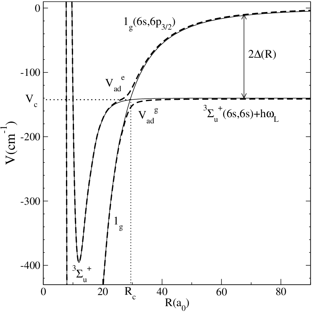
The photoassociation reaction is between two cold cesium atoms colliding in the ground state potential , at a temperature 0.11 mK, which are excited by a moderately strong laser pulse (with intensity I 43 MW/cm2) to form a molecule in a superposition of vibrational levels of the excited electronic potential . Only the wave of the collision is considered. For a rotational quantum number , the process can be schematized as:
| (1) |
The pulse is red-detuned with cm-1 from the energy of the D2 atomic transition (=- ). The large detuning determines a crossing of the field dressed diabatic potentials at the interatomic distance , with ===-143 cm-1 (figure 1).
The and electronic potentials used in the present calculation (figure 1) are built from quantum chemistry [20] and asymptotic calculations [21, 22] and were described in a previous paper [18].
2.1 Time-dependent model
The dynamics of the photoassociation process is simulated by solving numerically the time-dependent Schrödinger equation associated with the radial motion of the wavepackets and in the electronic channels and , coupled by an electric field with the amplitude . The equation can be written as [18]:
Equation (2.1) is obtained in the Born-Oppenheimer approximation for the diatomic molecule and using the rotating wave approximation with the frequency . The potentials and are the diabatic electronic potentials crossing in , represented in figure 1. is the kinetic energy operator and the coupling between the two channels, with the temporal envelope of the pulse. , where is the field amplitude (with the laser intensity), the polarization, and the transition dipole moment between the ground and the excited molecular electronic states. We neglect the R-dependence of the transition dipole moment, using the asymptotic value deduced from standard long-range calculations for a linear polarisation vector . This approximation remains good for the present calculation, as for distances around the crossing , the dipole moment is closed to its asymptotic value, 0.9 , and decreases slowly for smaller distances [23]. For a pulse intensity I 43 MW/cm2, the coupling becomes WL=13.17 cm-1, inducing a significant avoided crossing, as it can be seen in figure 1, where the light-induced or adiabatic potentials , are represented with dashed lines.
The numerical calculations were made for a rectangular pulse with a duration of 300 ps, whose envelope f(t) is represented in figure 2.

The Schrödinger equation (2.1) is solved by propagating in time an initial wavefunction on a spatial grid with the length a0. The time propagation uses the Chebychev expansion of the evolution operator [24, 25] and the Mapped Sine Grid (MSG) method [10, 27] to represent the radial dependence of the wavepackets.
The results extracted from the dynamics are:
- •
the evolution of the wavepackets during the pulse, for the two channels , , in the position representation, , and momentum representation, defined by the Fourier transforms ;
- •
the evolution of the population in each electronic state during the pulse. At a given instant , the population in one of the electronic states is calculated on the spatial grid extending from to , as:
(10) The spatial grid is chosen such as at every instant the total population is normalized at 1 on the grid (). At t=0 the population is entirely in the ground state ().
2.2 Time scales related to the laser coupling and vibrational movement
The time scales relevant for the dynamics are related to the laser coupling and to the vibrational movements in the electronic potentials. The spontaneous emission from the excited state is neglected, as the time evolution of hundreds picoseconds studied here is short compared with the spontaneous emission time of about 30 ns.
We begin by defining the characteristic times connected to the laser coupling.
A local time-dependent Rabi period can be associated with the laser coupling between the two electronic states [9]:
| (11) |
where 2 is the local detuning (see figure 1). Such a characteristic time is relevant if the impulsive approximation remains valid on the whole duration of the pulse, i.e. if the relative motion of the two nuclei can be considered as frozen during the pulse duration.
For the rectangular pulse studied here the coupling remains constant in the time interval (100 ps, 300 ps), so we can refer in the analysis at a local Rabi period associated to the constant coupling :
| (12) |
This local Rabi period has its maximum at the potentials crossing (=1.27 ps), diminishing with the increasing of the local detuning (for example =0.24 ps).
One can also associate a Rabi period with the beating induced by the coupling between two specific vibrational states, one belonging to the excited electronic state, and the other to the ground state. Indeed, in equation (2.1) the wavepackets can be developed as superpositions of vibrational wavefunctions with eigenenergies , corresponding to each electronic Hamiltonian ():
| (13) | |||
| (14) |
Supposing only two vibrational states, and , respectively, with , , , which are coupled by in equation (2.1), one obtains for the oscillating population in the excited state:
| (15) | |||
| (16) |
The corresponding Rabi period will depend on the overlap of the vibrational functions:
| (17) |
The time scale associated with the vibrational motion of a vibrational level with binding energy in an electronic potential is:
| (18) |
To estimate the coupling influence on the dynamics, the time scales (12) and (17) associated with the laser coupling shall be compared with the vibrational periods (18) of levels in the ground and excited potentials. In the case treated here, the Rabi periods associated with the laser coupling are of the order of picosecond, being much smaller than the characteristic vibrational periods implied in the problem (tens or hundred ps), which indicates a case of strong coupling [18].

2.3 Initial state: spatial and momentum representations
The representation of the initial state in a wavepacket treatment of the cold atoms photoassociation is discussed in [10]. For a low temperature collision (0.11 mK) and an excitation process taking place at short distances (), the initial state of the photoassociation process has to be represented using stationary collision states. We shall simulate the photoassociation dynamics using as initial state a continuum state of the ground electronic channel, having the energy . The results obtained can be used to estimate a photoassociation probability for an ensemble of cold atoms in thermal equilibrium at temperature (see Section 4).
In our numerical method, the initial continuum state is calculated as one of the eigenstates of the ground electronic state Hamiltonian, through the Sine Grid Representation [27], in a box of length . The method introduces a discretization of the continuum which supply continuum states having a node at the boundary of the box (as the sine basis functions used in representation). Then it is possible to have a continuum delocalized state as initial state in the wavepackets simulation of the photoassociation dynamics. The MSG method allows the use of large spatial grids on which the wavepackets dynamics in the range of distances relevant for the problem can be followed for long propagation times without being influenced by the external boundary of the box [10].
Here the initial state (see the (a) panel in figure 3) is chosen to be a continuum wavefunction of the (6s,6s) potential, of energy cm-1 corresponding to a temperature 0.11 mK. This wavefunction is calculated through the MSG method [27, 10] in the box of length a0, with a node at the end of the grid, and normalized to 1 on the grid. To obtain the normalization per unit energy the populations have to be multiplied by the density of states in the box at , [10]. The energy resolution for neighbouring eigenstates in the box at is cm-1, corresponding to =0.09 mK.

Figures 3(b) and (c) show the amplitude of the initial wavefunction in the momentum representation, . The wavefunction amplitude is mainly localized in the domain of “small momenta”, 0.06 a.u. (figure 3(c)), which corresponds to the large distances domain ( a0) in the position representation. A picture from the domain of “large momenta” ( 20 a.u.), where the wavefunction amplitude is much smaller, is displayed in figure 3(b). This domain of momenta corresponds to the domain of “small distances” in figure 3(a). We are interested to observe the changes appearing in both domains during the time evolution. The negative values mean momenta oriented to the inner wall of an electronic potential, and the positive values momenta oriented to large distances.

2.4 Wavepackets evolution during the pulse: spatial and momentum representations
The evolution of the wavepackets during the pulse is illustrated in figures 4 and 5, showing the and wavepackets in the spatial and momentum representations, respectively. The dynamics will be analysed in order to understand the vibrational movements inside each channel and the exchange of population between the electronic channels (figure 6).
In the potential, the excited wavepacket extends on the whole spatial grid, showing that bound and continuum levels are populated during the pulse. The vibrational movement of the population occupying bound states with outer turning points in the crossing region () can be well observed in the right columns of figures 4 and 5. The large amplitude of the wavepacket in the zone of big momenta (t=170, 250, 295 ps in the right column in figure 4) is equivalent with a strong presence of population at at the same moments. After the pulse, only bound levels remain populated in (figure 8 and section 4).
In the potential, the wavepacket moves progressively to the inner region (left column of figure 4). The vertical line in the same figure marks the separation in two spatial domains, which are differently affected by the pulse: at small and intermediate distances , the wavepacket is accelerated and deformed, but at large interatomic separations the action of the pulse can be considered as impulsive.
The wavepackets dynamics in the momentum representation (figure 5) makes visible an unexpected feature which appears from t=150 ps in the time evolution of the ground state wavepacket at a.u., and whose intensity increases until the end of the pulse. This result will be analysed in section 4.3.

3 Analysis of the population transfer during the pulse
We shall analyse the time evolution of the population transferred by the pulse in the excited state, , calculated with formula (10) and displayed in figure 6 (the population in the ground state has a complementary evolution, as , with ). The figure shows that from the large amount of population transferred during the pulse, which is of the order of , only remains at the end of the pulse. As it was discussed in the previous section, the large population transfer in the excited state during the pulse is related to the occupation of continuum states at large distances, in levels which do not rest populated after the pulse [9, 10]. On the contrary, what it is interesting for us is the population in bound vibrational levels, counting as cold molecules formation.
| (ps) | (cm-1) | (ps) | (cm-1) | (cm-1) | (ps) | |||
|---|---|---|---|---|---|---|---|---|
| 141 | 10.6 | -144.05 | 44 | 40 | -143.27 | 0.10 | 0.78 | 12.7 |
| 45 | 49 | -142.43 | 0.22 | 1.62 | 5.5 | |||
| 46 | 62 | -141.75 | 0.16 | 2.30 | 7 | |||
| 47 | 80 | -141.21 | 0.13 | 2.84 | 7.5 | |||
| 142 | 10.8 | -140.90 | 44 | 40 | -143.27 | 0.08 | 2.37 | 10.5 |
| 45 | 49 | -142.43 | 0.20 | 1.53 | 6 | |||
| 46 | 62 | -141.75 | 0.19 | 0.85 | 6.6 | |||
| 49 | 155 | -140.48 | 0.10 | 0.42 | 12.5 | |||
| 143 | 11 | -137.81 | 44 | 40 | -143.27 | 0.06 | 5.46 | 9 |
| 45 | 49 | -142.43 | 0.19 | 4.62 | 4.5 | |||
| 46 | 62 | -141.75 | 0.22 | 3.94 | 4.8 | |||
| 49 | 155 | -140.48 | 0.11 | 2.67 | 8.5 | |||
| 144 | 11.1 | -134.77 | 44 | 40 | -143.27 | 0.05 | 8.50 | 3.9 |
| 45 | 49 | -142.43 | 0.17 | 7.66 | 3.8 | |||
| 46 | 62 | -141.75 | 0.23 | 6.98 | 2.5 | |||
| 48 | 108 | -140.79 | 0.12 | 6.02 | 5 |
The vibrational levels of and predominantly populated by the pulse were identified by calculating the probabilities that a certain vibrational level of the excited or ground electronic state ( or ) to be populated at an instant . Two kinds of bound vibrational levels are mainly populated during the pulse in the state:
- •
levels around the crossing of the diabatic potentials: =141-144, with vibrational energies -144.5, -141.39, -138.29, -135.24 cm-1, lying in a domain of about 10 cm-1 containing the crossing energy cm-1, and with outer turning points of the vibrational wavefunctions lying around a0. These levels have vibrational periods of about 11 ps (see table 1).
- •
levels with ( cm-1), having vibrational wavefunctions lying at much larger distances ( a0). From these levels populated at large distances, only the levels 244 up to 248 remain notably populated after the pulse. Their vibrational periods are in the range 116 up to 130 ps.
The inset of figure 6 shows the evolution of in the time interval of constant coupling (between 100 ps and 295 ps). The oscillating features of during this time interval come from the exchange of population between vibrational levels of and located around the crossing (=141 up to 144 in the excited state, and =44 up to 49 in the ground state, see table 1), without major contribution from the population transferred at large distances. Indeed, as it is marked on the inset of figure 6, the energy domain covered by these oscillations is about , comparable with the final population in bound levels. Also, the variations of the total population between instants as t=130, 150, 170 ps, etc. are very closed to the variations of the population in levels around the crossing, given by the sum (t)=. Comparatively, the probability for the population of the levels =244-248, (t)=, shows much smaller variations.
The quantum beats appearing in figure 6 are related to the characteristic times of the dynamics: the vibrational movement in each potential well and the beating between the two coupled wavepackets, which are superpositions of vibrational functions corresponding to each electronic potential, as in (13) and (14). Table 1 gives a list of energies , vibrational periods , and characteristic beating times between levels in the ground and excited electronic states which contribute significantly in the exchange of populations between the two coupled channels; it also contains the overlaps with levels. Only the levels having the biggest overlaps with a given level are shown: these are the levels =44 up to 49, whose vibrational wavefunctions have the outer turning points at distances in the potential, and which are strongly populated by the pulse.
The population transfer between the two electronic channels is regulated by two time scales: a longer one, related to the vibrational movements inside the potential wells, and a shorter one, related to the Rabi coupling. The longer scale reflects the influence of the vibrational movements on the exchange of population between the two channels: the exchange is maximal when the amplitudes of the two wavepackets have a significant overlap, which, in the case of wavepackets vibrating in two different potential wells, arrives when both wavepackets have important localization probabilities in the crossing region [18]. When one of the wavepackets vibrates inside its potential, the transfer is generally diminished. The levels in the ground state have vibrational periods ( 40 ps) much longer than the levels in the excited state (about 11 ps). This explains the period of 40 ps appearing in the oscillations, which coincides with the vibrational period of the level =44 in the ground state, whose energy -143.27 cm-1 is very close to the crossing energy . On a much shorter scale, the transfer is guided by the strong laser coupling, which couples differently the implied levels. Table 1 shows characteristic times of beating (calculated with formula 17) varying from 2.5 to 12.7 ps for coupled pairs of vibrational levels in the ground and excited states. Comparing these times with the vibrational periods of the concerned levels, the strength of the coupling appears as varying very much among pairs of levels. The times scales given by are indicative for the short Rabi times appearing during the dynamics, for example the periods of 3 up to 4 ps of the fast oscillations in .
During the pulse the population accumulates in the state, such as in figure 6 appear not only the population beatings between the two channels, but also traces of the vibrational dynamics inside the excited potential: around t=250 ps, the two peaks of are separated by a time interval of 11 ps, which is the vibrational period of the levels located around the crossing: ps.
3.1 The light-induced (adiabatic) potentials

The mechanism of the population transfer during the pulse is enlightened if one analyses the light-induced (adiabatic) potentials. In figure 1 are represented both the diabatic potentials and the adiabatic ones, and , obtained from the diagonalization of the 2x2 potential matrix with constant coupling as non-diagonal term:
Expressions (3.1) and (3.1) illustrate the diabatic and adiabatic representations, respectively, of the operator. The coupling produces a strong deformation of the diabatic potentials around the crossing (figure 1), but its influence goes far beyond the crossing region, and this can be clearly seen if one compares the vibrational levels of the diabatic potentials with those of the adiabatic ones , . Such a comparison can be made using the series of rotational constants characterizing every potential. The energies and rotational constants were computed by solving numerically the corresponding stationnary Schrödinger equation using the Mapped Fourier Grid Hamiltonian (MFGH) method [26]. In figure 7 are represented the rotational constants as functions of the vibrational energies for and diabatic potentials, as well as for the adiabatic potentials , . We use the functions to observe how the energies of the vibrational levels in these potentials are distributed in a domain lying between -170 and -128 cm-1 around the crossing energy -143 cm-1. These results show that the influence of the coupling is strongly felt in a large energy domain of several tens of cm-1 around the crossing.
Also marked in figure 7 are the vibrational levels populated during the pulse and relevant to the dynamics, together with their vibrational periods. We shall focus on the levels located around the crossing region. The levels in the potential have vibrational periods ps. In the same energy region, the levels of the potential have bigger vibrational periods ps. Also, if the vibrational period of the levels located around the crossing, up to , is ps, in the adiabatic potential the levels belonging to the same energy domain have a vibrational period twice bigger: ps. Then, as it could be expected from the shape of the and (figure 1), the vibration in the adiabatic potentials is slowed down in the crossing region, influencing the population transfer between the two channels. The slowing down of the vibrational movement in the excited state lead to longer periods for the population exchange between the two channels and constitutes a mechanism for increasing progressively the population in the excited state.
The analysis of the adiabatic potentials can be used to extract characteristic times for the population exchange between the two channels. In an analogy with a two coupled states system, the Rabi beatings in the exchange of population is related to the Bohr frequency of the coupled system, which here can be found from the typical frequencies , connected with the new energies , of the levels in the coupled system. In figure 7 we show that for levels located in the crossing region such a characteristic time is about 45 ps, close to the period of ps of the large oscillations in figure 6.
4 Results at the end of the pulse
Figures 8 and 9 show the wavepackets (in position representation) and (in position and momentum representations) at the end of the pulse (t=395 ps). The main characteristics of the results will be discussed in the following.

4.1 Formation of strongly bound cold molecules in and electronic states
The strong coupling between the ground and excited states creates an interesting result at the end of the pulse: the population in bound levels of the ground state (mainly six levels, 47 up to 52), (t=395 ps)=2.83 10-4, is much bigger than the population photoassociated in the excited state, P(t=395 ps)=0.78 10-4. Some of the vibrational levels populated in , for example 47,48,49, have wavefunctions localized at distances a0, being then strongly bounded.
The final population in the excited state (figure 8) is entirely in bound vibrational states. A superposition of two kinds of vibrational levels is created, showing two mechanisms in the population transfer: at resonance, where mainly one level rests populated, =143 (with outer turning point at a0), whose population represents 82 P(t=395 ps), and off-resonance where several vibrational levels with outer turning points around a0 (=244 up to 248, representing P(t=395 ps)) are populated due to the strong coupling catching the large amplitude of the initial wavefunction between 45 and 65 a0 (figure 10). This last kind of transfer creates a hole in the ground state in this domain of interatomic distances, as it is indicated in figures 9(a) and 10. Such a result reflects the specificity of the present photoassociation conditions of strong field and large detuning.

The results obtained for a total population normalized at 1 on the grid allow an estimation of the averaged probability corresponding to a thermal distribution [10] at the temperature =0.11 mK, as:
| (25) |
where =P(t=395 ps)=0.78 10-4 is the probability obtained in the present calculation with an initial state of energy , is the density of states in the box of length at , is the Boltzmann constant, and is the partition function for a gas composed of non-interacting pairs of atoms in a volume (with the reduced mass of the diatom): . We then obtain and . For a number of atoms in a volume , and taking into account the spin degeneracy of the atomic state and of the initial electronic state, the total number of molecules photoassociated in per pump pulse is [10]: . For a volume =10-3 cm3 and a density of atoms =1011 atoms/cm3, the number of molecules obtained at the end of the pulse are: and .
4.2 Acceleration of the wavepacket to small interatomic distances
During the pulse, the slow packet is accelerated towards small interatomic distances R. The left column of figure 4 shows the time evolution of the wavepacket, which advances progressively to the inner zone. Especially the part of the wavepacket occupying distances R 70 a0 ¨feels¨ the acceleration to the crossing zone, where the diabatic potential in becomes the adiabatic one decreasing in (see figure 1). On the contrary, the maximum of the wavefunction located at R 89 a0 does not move during the pulse, but begin to be accelerated after the pulse. Similar observations can be made on figure 9 (a), showing the R-wavepacket at the end of the pulse (t=395 ps): the changes in the wavepacket amplitude are at distances R 89 a0. The momentum representation of the wavepacket at the same instant t=395 ps, in figure 9 (c), shows that, compared with the initial symmetric distribution (figure 3 c), the part corresponding to k0 has moved to bigger values, which also indicates the gain of kinetic energy in the electronic potential in the movement to small distances.
The creation of a “hole“ in the ground state wavepacket at the end of the pulse (discussed previously and shown in figure 9a)) is also a factor leading to a compression of population at short range, which after the pulse acts to increase the density of atom pairs at short distances [11].

4.3 Kinetic energy “gains” in the final wavepacket as signatures of the maxima in the initial wavefunction continuum
In this section we shall analyse some peculiar features appearing in the ground state wavepacket during the time evolution and at the end of the pulse (figure 9b)). The time evolution in the momentum representation (left column of figure 5), shows that, from t=150 ps, a line strikingly appears in the wavepacket amplitude , at k a.u. The kinetic energy associated with this momentum is cm-1, corresponding to the local difference in energy between and potentials at . The amplitude of the initial wavefunction has a maximum at this distance (figure 3 a), which does not move during the time evolution, but on which small oscillations begin to be superposed (see the left column of figure 4). The period of these oscillations is a0 , corresponding to a plane wave with a.u. The momentum width of this -feature in the wavepacket is a.u., which is consistent with the spread in distance on around R . We interpret this feature as corresponding to the kinetic energy of the population cycled back in the ground state from the excited state in the fast exchange of populations taking place around R due to the strong coupling between the two electronic channels, with =0.24 ps. At the end of the pulse, the line with k a.u. is accompanied in the wavepacket by its negative value a.u. (see figure 9b), which has to be a technical artefact coming from the propagation of this large positive momentum component to large interatomic R distances, followed by reflection at the end of the grid.
In fact, as it is shown in the Appendix, it seems that the momentum first appears associated with an ingoing plane wave travelling to small distances , but it is fast reflected by the inner wall of the potential and transformed in a positive travelling to large distances, which is easy to be observed in the wavepackets evolution. We have simulated the dynamics in the same conditions, but taking as initial wavepacket in the ground state a gaussian centered at R , and indeed we observed a peak at a.u. appearing early in the time evolution.
a.u. is not the only value of momentum for which a feature appears in the wavepacket. At various instants of the time evolution, other lines can be observed, at smaller values of . As these lines are embedded in the wavepacket, it becomes easier to distinguish them for larger momenta where the wavefunction amplitude is smaller. In figure 9b, showing the wavepacket amplitude in the domain of large momenta, at the end of the pulse, other lines can be observed at the values: k=12.2, 10.4, 8.6 and 6 a.u. They correspond to kinetic energies =134.8, 98, 68.6 and 32.6 cm-1. If one associates these kinetic energies to local differences between the electronic potentials, then, according to the reasoning just exposed they correspond to local transitions from the excited to the ground state taking place at distances R 89, 43.9, 36.8 and 32 a0, where maxima of the initial wavefunction are located, as it appears in figure 10. Other local maxima of the initial wavefunction, at R=47 a0 and 59 a0, do not have a correspondent k-value in the final momentum distribution of the ground state wavepacket, but in this domain of distances the population is not cycled back to the ground state, remaining transferred to the levels =244 up to 248 of the excited state (see figure 8). As a consequence, as we showed already, a hole is created in the ground state in this spatial domain (figure 9a).
We also have to mention that for longer propagation times one can see appearing in the wavepacket peaks corresponding to the negative values of these other smaller momenta: -10.4, -8.6 and -6 a.u.
In the Appendix we use the impulsive approximation in the limit to show the emergence of such momenta during the time evolution. Indeed, as we emphasized, for the maximum of the ground wavefunction located at R , the impulsive approximation rests valid during the whole pulse (see figure 9a), and for other maxima the impulsive approximation could be applied on smaller durations of the pulse.
The significant fact is that these “large momenta“ appearing at the end of the pulse in the ground state wavepacket are signatures of the maxima in the initial wavefunction continuum. This is a specific effect of the strong photoassociation pulse applied at small distances which reveals the structure of the initial ground state.
5 Comments and Conclusions
We have analysed the dynamics in the photoassociation of a pair of cold atoms by a strong laser pulse (I 43 MW/cm2) applied at short interatomic distances () for a cold collision. The numerical calculations were made for the transition in Cs2, at a temperature 0.11 mK. The large detuning ( cm-1) and the intensity of the pulse were chosen to correspond to a specific regime imposed by the limit of an asymptotic detuning much bigger than the maximum of the coupling, cm-1 cm-1, in order to avoid the transfer of population to the continuum of the excited state at the end of the pulse.
The specificity of this regime comes from two sides: a) the large detuning which locates the resonance condition at small or intermediate interatomic distances, making “visible” the nodal structure of the initial continuum wavefunction; b) the strong coupling between the two electronic channels, which acts not only on vibrational levels around the crossing of the dressed electronic potentials, but also induces off-resonance cyclings of population between the coupled electronic states.
We have chosen not only a quite strong pulse, but also a quite long one (a rectangular pulse of about 300 ps), in order to obtain a better understanding of the time evolution in the presence of the pulse and to see how efficient for the cold molecule formation is the acceleration of the population from large to small interatomic distances.
In this strong regime of coupling, the photoassociation dynamics during the pulse takes place in the light-induced (adiabatic) potentials, whose topology influence the exchange of population between the coupled channels. In our example, the shapes of the adiabatic potentials lead to acceleration of the ground state population to the inner region (at short distances the diabatic potential in becomes the adiabatic one decreasing in ), and also to the slowing down of the vibrational movement in the crossing region, which is a mechanism for increasing progressively the population in the excited state.
The main characteristics of the results at the end of the pulse are the following:
(i) It appears that such a pump scheme allows for the production of ground state molecules through a single laser pulse. Indeed, strongly bound cold molecules are formed in and electronic states, the population transferred in bound levels of the ground state being much bigger than the population photoassociated in bound levels of the excited state. Some of the vibrational levels populated in have wavefunctions localized at distances a0. The final population in the excited state is entirely in bound vibrational levels, populated both at resonance (, with outer turning point at a0) and off-resonance, where several vibrational levels with outer turning points around a0 are populated due to the strong coupling catching the large amplitude of the initial wavefunction between 45 and 65 a0. This last kind of transfer creates a hole in the ground state in this domain of interatomic distances.
(ii) During the pulse the population in the ground state is globally accelerated towards small interatomic distances. The creation of a “hole“ in the ground state wavepacket at the end of the pulse is also a factor leading to a compression of population at short distances [11].
(iii) At the end of the pulse, the momentum distribution of the ground state wavepacket keeps the traces of the initial continuum maxima. This is an effect of the strong coupling leading to off-resonance cycling of population between the two channels and bringing kynetic energy in the ground state. The cycling of population is particularly important at those interatomic distances where the maxima of the initial continuum are located.
An important question is if the regime explored here can be mantained if, for example, one increases the detuning , in order to form cold molecules in lower vibrational levels of the ground state. An insight about the results which can appear by increasing the detuning can be extracted in the impulsive limit, which normally rests valid at large interatomic separations. In the impulsive limit, the population in the excited state at the end of the pulse can be approximated as [24]:
| (26) |
where (for , ). Equation (26) shows that the transfer from the ground to the excited state is favoured: a) at large interatomic distances R, because is the amplitude of an initial continuum wavefunction of low energy in the ground state; b) at resonance (); c) for a strong coupling , when, depending on the ratio and the pulse duration, various ranges of distances can be populated. It has to be observed that, increasing the detuning , one increases , so the oscillations in with the period will be very fast and produce an unstable regime of transfer, in which the result at the end of the pulse cannot be predicted. In this regime, the large distances and the continuum of the excited state can easily rest populated after the end of the pulse. The only manner to overcome these difficulties is to increase the coupling, which can broke the impulsive limit and bring population to short distances. Then, the ratio is indeed a significant parameter for the regime explored here, which can be maintained for a larger detuning only if the pulse intensity is also increased.
The acceleration of the population to the inner region and the efficiency in forming strongly bound cold molecules is related here to a non-impulsive regime of coupling brought at a0 by the strength and the time duration of the pulse.
These results have to be completed with a further investigation of the time evolution subsequent to the pulse. Also the model can be enriched by considering couplings with other electronic surfaces. Our work is a tentative to show that the photoassociation of cold atoms at small/intermediate distances with an intense laser pulse offers the possibility to explore cold molecules formation using the specific topologies of the light-induced potentials. Favorable conditions can be found taking into account the variety of electronic transitions in alkali dimers which can be controlled by the parameters of the photoassociation pulse.
Appendix: Kinetic energy “gains” in the ground state due to the off-resonance cycling of population between the strongly coupled electronic states.

We shall consider the time-dependent Schrödinger equation (2.1) for constant coupling . In [28] it is shown that, if the impulsive approximation is valid at a given R, the wavefunction on the ground state surface after a time becomes:
| (27) |
where is the energy corresponding to the initial stationnary wavefunction at t=0 (), 2 is the local detuning, the spatial dependent Rabi pulsation:
| (28) |
and
| (29) |
We calculated numerically the time-dependent prediction for the ground state wavefunction in the impulsive approximation, , using (27). In figure 11 we show the corresponding momentum distribution at t=300 ps, , which indeed displays peaks at values deduced from the maxima of the initial wavefunction, according to the discussion of Section 4.3.
In the following we shall introduce approximations into (27) in order to make appear analitically a momentum associated with a maximum of the initial wavefunction at .
In (27), represents a free evolution in the ground state. The factor superposed on this free evolution can be separated:
| (30) | |||||
| (31) |
We shall make approximations on the expression (31) in the limit . Indeed, this limit is valid at , where cm-1, and cm-1. Then it is possible to approximate:
| (32) |
Consequently, at a given R value where the impulsive approximation is valid, can be decomposed in two terms:
| (33) | |||
| (34) | |||
| (35) |
For the first term is the dominant one. Indeed, a rough approximation implies , the second term having an incomparable smaller contribution (). It is the second “small” term which offers the explanation for the “k- features” observed in our results. Its Fourier transform is:
| (36) | |||
| (37) |
with . We shall take into account only the contribution at the integral coming from a small domain of R, , around the point , assuming that on this domain is a Gaussian of width centered in : , and that depends linearly on R near : . Then:
| (38) | |||||
where and the initial domain of integration was taken from to . For a sufficiently large, the integral in (38) becomes a function, such as:
| (39) | |||||
In (39) one can see appearing the contribution of an ingoing () plane wave , of energy and momentum [29]. The function shows that this momentum = is related to the local energy difference between the electronic potentials at , or that . If one associates this momentum to the movement of an ingoing particle of mass , , then one obtains , and finally .
Then indeed (39) makes appear a momentum connected to , as we observed in our results discussed in Section 4.3, and oriented to small R distances. The fact that we first observe an outgoing wave has to be due to the rapid reflection of the ingoing waves by the inner wall of the ground state potential.
An estimation of the wavefunction amplitude for using formula (39) gives . This qualitative estimation obtained analitically for unprecised corresponds to the amplitudes calculated numerically for 12.2 a.u., from the dynamics and in the impulsive approximation, which are in agreement: 0.004 (see figure 9b) and figure 11).
References
References
- [1] Jones K M, Tiesinga E, Lett P D and Julienne P S 2006 Rev. Mod. Phys. 78 483
- [2] Salzmann W et al. 2006 Phys. Rev. A 73 023414
- [3] Brown B L, Dicks A J and Walmsley I A 2006 Phys. Rev. Lett. 96 173002
- [4] Wright M J, Pechkis J A, Carini J L and Gould P L 2006, Phys. Rev. A 74 063402
- [5] Wright M J, Pechkis J A, Carini J L, Kallush S, Kosloff R and Gould P L 2007 Phys. Rev. A 75 051401(R)
- [6] Veshapidze G, Trachy M L, Jang H U, Fehrenbach C W and DePaola B D 2007 Phys. Rev. A 76 051401(R)
- [7] Weise F et al. 2007 Phys. Rev. A 76 063404
- [8] Vala J, Dulieu O, Masnou-Seeuws F, Pillet P and Kosloff R 2001 Phys. Rev. A 63 013412
- [9] Luc-Koenig E, Kosloff R, Masnou-Seeuws F and Vatasescu M 2004 Phys. Rev. A 70 033414
- [10] Luc-Koenig E, Vatasescu M and Masnou-Seeuws F 2004 Eur. Phys. J. D. 31 239
- [11] Luc-Koenig E, Masnou-Seeuws F, and Kosloff R 2007 Phys. Rev. A 76 053415
- [12] Koch C P, Luc-Koenig E and Masnou-Seeuws F 2006 Phys. Rev. A 73 033408
- [13] Koch C P, Kosloff R and Masnou-Seeuws F 2006 Phys. Rev. A 73 043409
- [14] Mur-Petit J, Luc-Koenig E and Masnou-Seeuws F 2007 Phys. Rev. A 75 061404(R)
- [15] Kallush S and Kosloff R 2007 Phys. Rev. A 76 053408
- [16] Shapiro E A, Shapiro M, Pe’er A and Ye J 2007, Phys. Rev. A 75 013405
- [17] Shapiro E A, Pe’er A, Ye J, and Shapiro M 2008 Phys. Rev. Lett. 101 023601
- [18] Vatasescu M, Dulieu O, Kosloff R, and Masnou-Seeuws F 2001 Phys. Rev. A 73 033407
- [19] Vatasescu M 2008 Nucl. Instr. and Meth. in Phys. Res. B doi:10.1016/j.nimb.2008.10.033
- [20] Spies N 1989 Ph.D. Thesis Universität Kaiserslautern
- [21] Marinescu M and Dalgarno A 1995 Phys. Rev. A 52 311
- [22] Marinescu M and Dalgarno A 1996 Z. Phys. D 36 239
- [23] Vatasescu M 1999 Ph. D. Thesis Université Paris XI
- [24] Kosloff R 1994 Annu. Rev. Phys. Chem. 45 145
- [25] Kosloff R 1996 Quantum Molecular Dynamics on Grids Dynamics of Molecules and Chemical Reactions ed R E Wyatt and J Z Zhang (New York: Marcel Dekker) pp 185-230
- [26] Kokoouline V, Dulieu O, Kosloff R and Masnou-Seeuws F 1999 J. Chem. Phys. 110 9865
- [27] Willner K, Dulieu O and Masnou-Seeuws F 2004 J. Chem. Phys. 120 548
- [28] Banin U, Bartana A, Ruhman S and Kosloff R 1994 J. Chem. Phys. 101 8461
- [29] Messiah A 1969, Mécanique Quantique (vol 1) (Paris: Dunod)