Inflation and Reheating in Induced Gravity

Beginning with the association of the gravitational coupling with a scalar field [1] many attempts have been made to relate the gravitational constant to dynamics. Indeed starting from an attempt to relate it to one loop effects in some fundamental interaction [2] induced gravity (IG) theories $\gamma\sigma^{2}R$ have been developed [3, 4, 5]. In such theories $\sigma$ acquires a non zero vacuum expectation value through the spontaneous breaking of scale invariance arising through the presence of a condensate [3] or quantum effects (radiative corrections) [6]. Further such theories can be generalized [7] leading to a viable dark energy model [8].
In IG one may also use $\sigma$ to achieve inflation. “Old inflation” in such a context is not satisfactory [9] and small field and large field (chaotic) inflation appear more promising. In particular for the last case with $\gamma\gg 1$ the constraints on $\sigma$ are such that it may even be compatible with spontaneous symmetry breaking in the usual particle physics context [10, 11, 12].

In this Letter we analyze the slow-roll predictions for single-field inflation in IG and compare them with the recent WMAP 5-yrs data [14]. We also give an analytic approximate solution for the coherent oscillation regime during which reheating in IG takes place.

Let us start by considering the IG action

$$S=\int d^{4}x\sqrt{-g}\left[{\gamma\over 2}\sigma^{2}R-\frac{g^{\mu\nu}}{2}\partial_{\mu}\sigma\partial_{\nu}\sigma-V(\sigma)\right]$$

(1)

where $\gamma$ is a dimensionless and positive definite parameter and we assume a spatially flat Robertson-Walker background. The variation of the above action leads to the following set of independent equations

	$\displaystyle H^{2}$	$\displaystyle=$	$\displaystyle\frac{1}{3\gamma\sigma^{2}}\left[\frac{\dot{\sigma}^{2}}{2}+V(\sigma)\right]-2H\frac{\dot{\sigma}}{\sigma}$		(2)
	$\displaystyle\ddot{\sigma}$	$\displaystyle+$	$\displaystyle 3H\dot{\sigma}+\frac{\dot{\sigma}^{2}}{\sigma}=-\frac{V_{\mathrm{eff},\sigma}}{1+6\gamma}$		(3)

where $V_{\mathrm{eff},\sigma}={\rm d}V/{\rm d}\sigma-4V/\sigma$ and the dot is the derivative with respect to cosmic time.

Inflation generically occurs during the slow-rolling of $\sigma$, for which Eqs. (2,3) reduce to:

$$H^{2}\simeq\frac{V}{3\gamma\sigma^{2}}\mbox{,}\quad 3H\dot{\sigma}\simeq-\frac{V_{\mathrm{eff},\sigma}}{1+6\gamma}$$

(4)

The slow-roll parameter $\epsilon_{1}\equiv-\dot{H}/H^{2}$ obtains contributions not only from the square of the velocity of the scalar field as in EG but also from other terms:

$$\dot{H}=-\frac{1}{2\gamma}\frac{\dot{\sigma}^{2}}{\sigma^{2}}+4H\frac{\dot{\sigma}}{\sigma}+\frac{V_{\mathrm{eff},\sigma}}{\sigma(1+6\gamma)}$$

(5)

As in Einstein Gravity (EG), it is useful to introduce the hierarchy of Hubble flow functions [15]: $d\ln\epsilon_{n}/dN=\epsilon_{n+1}$ with $n\geq 0$, $\epsilon_{0}=H_{i}/H$ and $N$ being the number of e-folds. In scalar-tensor gravity it is also necessary to introduce another hierarchy associated with $\sigma$: $d\ln\delta_{n}/dN=\delta_{n+1}$ with $n\geq 0$, $\delta_{0}=\sigma/\sigma_{i}$. Thus in IG the cosmological perturbations depend on these two hierarchies which completely specify the background evolution. As usual, one can replace equations (2,3) with an equivalent set written in terms of the two hierarchies. However the two hierarchies are not independent and the following relation holds:

$\displaystyle\epsilon_{1}$

$\displaystyle=$

$\displaystyle\frac{\delta_{1}}{1+\delta_{1}}\left(\frac{\delta_{1}}{2\gamma}+2\delta_{1}+\delta_{2}-1\right)$

(6)

Inflation in IG has a richer phenomenology than in EG: inflation could occur for large $\delta_{1}$ and a super-inflationary stage [17] could take place for $|\delta_{1}|\ll 1$, ($\epsilon_{1}=-\dot{H}/H^{2}<0$) in the Jordan frame with $\delta_{1}>0$ and $2\delta_{1}+\delta_{2}+\delta_{1}/(2\gamma)<1$ or viceversa.

Scalar curvature perturbations produced by quantum fluctuations of the inflaton during the accelerated stage are described by $\mathcal{R}(x)=-H\delta\sigma(x)/\dot{\sigma}$ in the uniform curvature gauge [16], where $\delta\sigma(x)$ is the scalar inflaton perturbation and is the correct field variable to quantize. The Fourier component $\delta\sigma_{k}$ of the inflaton fluctuation, in the IG context, has been shown to satisfy the differential equation [16]:

	$\displaystyle\ddot{\delta\sigma_{k}}$	$\displaystyle+$	$\displaystyle\left(3H+\frac{\dot{Z}}{Z}\right)\dot{\delta\sigma_{k}}+$		(7)
		$\displaystyle+$	$\displaystyle\left[\frac{k^{2}}{a^{2}}-\frac{1}{a^{3}Z\sigma\delta_{1}}\left(a^{3}Z\left(\sigma\delta_{1}\right)^{\cdot}\right)^{\cdot}\right]\delta\sigma_{k}=0$

where

$$Z=\frac{H^{2}\sigma^{2}(1+6\gamma)}{(\dot{\sigma}+H\sigma)^{2}}=\frac{1+6\gamma}{(1+\delta_{1})^{2}}.$$

(8)

Gravitational waves are also amplified from quantum fluctuations during inflation; in IG the Fourier modes of tensor perturbations satisfy:

$$\ddot{h}_{s,k}+(3H+2H\delta_{1})\dot{h}_{s,k}+\frac{k^{2}}{a^{2}}h_{s,k}=0$$

(9)

where $s=+\,,\times$ denotes the two polarization states. We define the power spectra of scalar curvature perturbations and tensor perturbation as

$$\mathcal{P}_{\mathcal{R}}(k)\equiv\frac{k^{3}}{2\pi^{2}}|\mathcal{R}_{k}|^{2}\simeq\mathcal{P}_{\mathcal{R}}(k_{*})\left(\frac{k}{k_{*}}\right)^{n_{s}-1}$$

(10)

and

$$\mathcal{P}_{h}(k)\equiv\frac{2k^{3}}{\pi^{2}}\left(|h_{+,k}|^{2}+|h_{\times,k}|^{2}\right)\,\simeq\mathcal{P}_{h}(k_{*})\left(\frac{k}{k_{*}}\right)^{n_{t}}$$

(11)

respectively, where $k_{*}$ is a suitable pivot scale. It is important to stress that through a conformal transformation the action in Eq. (1) can be rewritten as EG involving the rescaled scalar field and metric with a different potential: whereas the spectra of primordial cosmological perturbations are conformal invariant, we prefer to work in the original frame in Eq. (1).

As in EG with a standard scalar field with exponential potential, exact inflationary solutions with $a(t)\sim t^{p}$ (with $t>0$ and $p>1$) exist for induced gravity with $V(\sigma)=\lambda_{n}\sigma^{n}/n$ and

$\displaystyle p=\frac{1}{\epsilon_{1}}=2\frac{1+(n+2)\gamma}{(n-4)(n-2)\gamma}\,,\,\,\,\,\sigma(t)=\frac{S}{t^{\frac{2}{(n-2)}}}\,,$

(12)

with $4<n<4+\sqrt{2(6+1/\gamma)}$ or $4-\sqrt{2(6+1/\gamma)}<n<2$ [18]. These are scaling solutions for which $\delta_{2}=0$ and

$$\delta_{1}=-\frac{\gamma\left(n-4\right)}{1+\gamma\left(n+2\right)},\;\;\epsilon_{1}=\frac{\gamma\left(n-2\right)\left(n-4\right)}{2+2\gamma\left(n+2\right)}\,.$$

(13)

The poles in $n=2\,,4$ in the above equations correspond to de Sitter solutions having $a(t)\propto e^{Ht}$. The above scaling solution is also found for $a(t)\sim(-t)^{p}$ (with $t<0$ and $p<0$) but only for $2<n<4$: this solution characterizes a super-inflationary stage with $\dot{H}>0$ and ends up in a future singularity (the Ricci scalar grows with the arrow of time instead of decreasing). Let us note that inflation does not end for the above scaling solutions (just as in EG), but cosmological perturbations can be solved exactly on such backgrounds. The spectral index for scalar curvature perturbations is:

$$n_{s}-1=\frac{{\rm d}\ln\mathcal{P}_{\mathcal{R}}}{{\rm d}\ln k}=\frac{2\gamma\left(n-4\right)^{2}}{\gamma\left(n-4\right)^{2}-2\left(6\gamma+1\right)}$$

(14)

where ${\rm d}n_{s}/{\rm d}\ln k={\rm d}n_{t}/{\rm d}\ln k=0$ and $n_{t}=n_{s}-1$. The exact tensor-to-scalar ratio is given by

$$r=\frac{\mathcal{P}_{h}(k)}{\mathcal{P}_{\mathcal{R}}(k)}=-\frac{8n_{t}}{1-\frac{n_{t}}{2}}$$

(15)

which agrees with the consistency condition of power-law inflation in EG. On examining the behavior of (14) one has

$$n_{s}-1<0\quad{\rm when}\quad\rho\equiv\frac{\gamma\left(n-4\right)^{2}}{2(1+6\gamma)}<1\,$$

(16)

and $n_{s}-1$ is close to scale invariance (zero) only for $\rho\sim 0$ and $n_{s}-1>2$ for $\rho>1$.

Let us now obtain general formulae for scalar and tensor spectra in the slow-roll regime. As for EG, the potential and its derivatives are given explicitly by the Hubble parameter and the coefficients of the hierarchies $(\epsilon_{i},\delta_{i})$. On assuming $\delta_{i}\ll 1$, we can invert such relations obtaining (we only exhibit the first two):

	$\displaystyle\delta_{1}$	$\displaystyle\simeq$	$\displaystyle-\gamma\sigma\frac{V_{\mathrm{eff},\sigma}}{(1+6\gamma)\,V}\,,$		(17)
	$\displaystyle\delta_{2}$	$\displaystyle\simeq$	$\displaystyle-\gamma\sigma^{2}\frac{V_{\mathrm{eff},\sigma\sigma}}{(1+6\gamma)\,V}+\delta_{1}\left(\frac{\delta_{1}}{\gamma}-3\right)\,.$		(18)

From eq. (17) we immediately see that the first slow-roll parameter in IG is roughly the square root of what we expect from EG. Indeed through a conformal trasformation to the Einstein frame one can show that $\epsilon_{1}^{\rm EF}=\delta_{1}^{2}(1+6\gamma)/(2\gamma(1+\delta_{1})^{2})$. Further, from Eq. (17), it is easy to see that $\epsilon_{1}\simeq-\delta_{1}$ to lowest order for large $\gamma$. The scalar power-spectrum is

$$\mathcal{P}_{\mathcal{R}}(k_{*})\simeq\frac{A\,H^{2}_{*}}{4\pi^{2}\left(1+6\gamma\right)\delta_{1\,*}^{2}\sigma_{*}^{2}}\simeq\frac{A\,V^{3}_{*}(1+6\gamma)}{12\pi^{2}\gamma^{3}\sigma_{*}^{6}V^{{}^{\prime}2}_{\mathrm{eff}\,*}}$$

(19)

with

$$A=\left[1-2\epsilon_{1\,*}+C\left(\delta_{1\,*}+\delta_{2\,*}+\epsilon_{1\,*}\right)\right],$$

(20)

where $C=2\left(2-\ln 2-b\right)$, $b$ is the Euler-Mascheroni constant and all the above quantities with the subscript $*$ are evaluated when $k_{*}$ crosses the Hubble radius. The scalar spectral index in Eq. (10) is

	$\displaystyle\!\!\!\!\!\!\!n_{s}-1$	$\displaystyle=$	$\displaystyle-2\left(\delta_{1\,*}+\delta_{2\,*}+\epsilon_{1\,*}\right)$		(21)
		$\displaystyle=$	$\displaystyle\frac{2\gamma\,\sigma_{*}^{2}}{1+6\gamma}\left(\frac{V_{\mathrm{eff},\sigma\sigma*}}{V_{*}}-\frac{3V_{\mathrm{eff},\sigma*}^{2}}{2V_{*}^{2}}-\frac{3V_{\mathrm{eff},\sigma\,*}}{\sigma_{*}V_{*}}\right)$

Let us note that the above result for $n_{s}$ agrees with the calculation in the Einstein frame, but does not agree with Ref. [19] where a term of order $\delta_{i}$ is omitted. We also note $V_{\mathrm{eff}\,,\sigma}$ is less than $V$ to the addition of radiative corrections of logarithmic form to the tree potential.
Similarly, the tensor power spectrum is given by:

$$\mathcal{P}_{h}(k_{*})\simeq\frac{2(A-C\delta_{2\,*})H_{*}^{2}}{\pi^{2}\gamma\sigma_{*}^{2}}\simeq\frac{2(A-C\delta_{2\,*})V_{*}}{3\pi^{2}\gamma^{2}\sigma_{*}^{4}}$$

(22)

and

$$n_{t}\simeq-2\left(\delta_{1*}+\epsilon_{1*}\right)\simeq-\frac{\delta_{1\,*}^{2}(1+6\gamma)}{\gamma}\,.$$

(23)

The above results lead to the standard tensor-to-scalar ratio $r_{*}\simeq-8n_{t*}$. We shall consider the following potentials leading to the spontaneous breaking of scale invariance and Newton’s constant:

$$V_{\rm CW}=\frac{\mu}{8}\sigma^{4}\left(\ln\frac{\sigma^{4}}{\sigma_{0}^{4}}-1\right)+\frac{\mu}{8}\sigma_{0}^{4}$$

(24)

where the breaking arises through a quantum effect, Coleman-Weinberg (CW) type, and

$$V_{\rm LG}=\frac{\mu}{4}\left(\sigma^{2}-\sigma_{0}^{2}\right)^{2}\,.$$

(25)

where the breaking arises through a condensate, Landau-Ginzburg (LG) type.

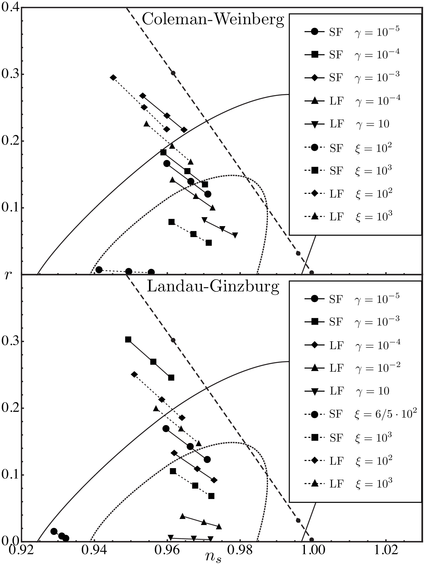
Both large and small field configurations for the potentials (24,25) can lead to predictions in agreement with observations, for suitable values of $\gamma$ and the parameters of the potential, $\mu\,,\sigma_{0}$. In Figure (1) we plotted the values of $(\sigma^{*},\gamma)$ in the small field regime and assuming that $k_{*}=aH$ for 50-70 e-folds, $N_{*}$, before inflation ends. Lighter regions represent the observational constraints on the spectral index $n_{s}$ coming from the WMAP 5 + BAO + SN Ia and a $68\%$ and $95\%$ confidence level ($n_{s}=0.963\pm 0.014$ and $n_{s}=0.963\pm 0.028$), darker regions represent the two intervals $50<N_{*}<60$ and $60<N_{*}<70$ (darker area). Such a plot constraints $\gamma$ to be $\lesssim 3\cdot 10^{-3}$ in order to fit observations. We note that small field regime in IG leads to predictions very different from EG. For both CW and LG potentials we obtain $n_{s}-1\simeq-16\gamma/(1+2\gamma)$. For small field potentials as $V(\sigma)\propto 1-(\sigma/\sigma_{0})^{n}+...$ we obtain $n_{s}-1\simeq-16\gamma/(1+6\gamma)$. For large field configurations, we obtain $n_{s}-1\simeq-2/N_{*}\,\,(n_{s}-1\simeq-1.5/N_{*})$ for LG (CW) which leaves $\gamma$ unconstrained. The amplitude for scalar perturbations for the LG potential is

$$P_{\mathcal{R}}(k*)\simeq\left\{\begin{array}[]{lcl}\frac{\mu}{3\pi^{2}\gamma}N_{*}^{2}\mbox{,}&\gamma\ll 1&(\mbox{large and small field})\\ \frac{\mu}{72\pi^{2}\gamma^{2}}N_{*}^{2}\mbox{,}&\gamma\gg 1&(\mbox{large field})\end{array}\right.\,.$$

(26)

WMAP5 + BAO + SN Ia require $P_{\mathcal{R}}(k^{*})=(2.445\pm 0.096)\times 10^{-9}$ [14]: from the above expression we observe that when $\gamma\gg 1$ $\mu$ need not be as small as the same self-coupling in EG[10, 11, 12]. For instance $\mu\sim 0.5$ is allowed for $\gamma\simeq 3\times 10^{4}$; on requiring $\gamma\sigma_{0}^{2}=M_{\rm pl}^{2}$, it is clear that in general IG can incorporate the GUT symmetry breaking scale for inflation.

In Figure (2) we compared the WMAP5+BAO+SN Ia constraints at the 68% (dotted contour) and the 95% (continuous contour) confidence levels [14] with the prediction for the potentials (24,25) both in IG (continuous lines) and in EG (dashed lines) framework: each point represents a different choice for $\gamma$ (or $\xi\equiv\sigma_{0}^{2}/{\rm M_{\rm P}}^{2}$ in EG) and $N_{*}$ (identical markers, from left to right, identify $N_{*}=50,60,70$). We observe that in IG for both the above potentials, the small field inflation with $\gamma\geq 10^{-3}$ is disfavoured by observations confirming what was found in the $n_{s}$ analysis. Again large field inflation in IG fits observations independently of $\gamma$ in contrast with the same regime in EG which requires $\xi\geq 10^{3}$. It is however worth noting that both the potentials (24,25), although very similar to a simple quartic potential in this regime, fit observations well, independently of $\mu$ and $\sigma_{0}$, in contrast with such a potential in EG which leads to results lying far away from the 95% region in the same e-folds interval.

Let us now study the oscillating regime occuring for $\sigma\simeq\sigma_{0}$ and consider the symmetry-breaking potential in Eq. (25) for the sake of simplicity. We find an approximate analytic solution given by:

	$\displaystyle\sigma(t)$	$\displaystyle=$	$\displaystyle\sigma_{0}+\frac{2}{t}\sqrt{\frac{\gamma}{3\mu}}\sin\left(\omega t\right)+\mathcal{O}\left(\frac{1}{t^{2}}\right)$		(27)
	$\displaystyle H(t)$	$\displaystyle\simeq$	$\displaystyle\frac{2}{3t}\left[1-\sqrt{\frac{6\gamma}{1+6\gamma}}\cos\left(\omega t\right)\right]+\mathcal{O}\left(\frac{1}{t^{2}}\right)\,,$		(28)

where $\omega=\sigma_{0}\sqrt{2\mu/(1+6\gamma)}$. On fixing the Planck mass after inflation by $M_{\rm pl}^{2}=\gamma\sigma_{0}^{2}$ and requiring curvature perturbations in agreement with observations, the frequency of oscillations $\omega$ is $\simeq 2.5\times 10^{13}$ GeV for $\gamma\ll 1$ (and twice as large for $\gamma\gg 1$). For the regime of small oscillations this study is equivalent to a mass term obtained from the oscillations of $\sigma$ around a minimum of a potential with $V(\sigma_{0})=0$.

Eqs. (28) can be used to study the evolution of $\delta\sigma$ during the coherent oscillations of $\sigma$: on using Eq. (7) the variable $\tilde{\delta\sigma_{k}}=\sqrt{a^{3}Z}\delta\sigma_{k}$ can be recast in a Mathieu-like form:

$$\frac{d^{2}\tilde{\delta\sigma_{k}}}{d(\omega t)^{2}}+\left[A(t)+2q_{1}(t)\sin\left(2\omega t\right)+2q_{2}(t)\sin\left(\omega t\right)\right]\tilde{\delta\sigma_{k}}=0$$

(29)

analogously to the EG case [22]. The leading terms in $q_{1}$ and $q_{2}$ originate from the metric and the potential contributions respectively, and both decay as $1/t$, further $A(t)=k^{2}/(a^{2}\omega^{2})+1+{\cal O}(t^{-2})$. Because of the two oscillating terms the time dependent frequency in Eq. (29) leads to beats. We obtain $q_{2}=\sqrt{27\gamma/(2(1+6\gamma))}/(\omega t)$ and $q_{1}=2/(\omega t)$ (the latter is the same as the EG case [22]).

The consequence of coherent oscillations on $\tilde{\delta\sigma_{k}}$ differs from the resonance for test scalar fields coupled to a massive inflaton [23], for which $q(t)$ ($\sim{\cal O}(t^{-2})$) decays faster than $k^{2}/a^{2}$ and as a consequence the resonance shuts-off asymptotically for large times although it started in the broad regime. According to Eq. (29), all wavelengths end asymptotically in the first resonance band since $q(t)$ decays more slowly than $k^{2}/a^{2}$. Thus for short-scale modes with $H\ll k/a\ll\omega$, $\delta\sigma_{k}$ oscillates with a constant amplitude instead of decaying [21]. Note that such a gravity mediated self-decay of the inflaton in its short-scale fluctuations also exists for $V(\phi)=m^{2}\phi^{2}/2$ or for a potential with a symmetry-breaking term in EG [24]. Although oscillating terms decaying as $1/t$ appear in the equation for gravitational waves - on rewriting Eq. (9) in terms of the variable $a^{3/2}\sigma h_{k}$ - such terms do not affect the standard behaviour of short-scale gravitational waves.
It is also interesting to study a possible connection of this inflationary stage with the problem of dark energy, which can also be modelled in IG through simple potentials [7, 8]. Work in this direction is in progress [21].

Acknowledgement. FF wishes to thank Jerome Martin and Karsten Jedamzik for discussions on preheating.

References

- [1] C. Brans and R. H. Dicke, Phys. Rev. 124 (1961) 925.
- [2] A. D. Sakharov, Dokl. Akad. Nauk. SSSR 117, 70 (1967); [Sov. Phys. Dokl. 12, 1040 (1967)].
- [3] A. Zee, Phys. Rev. Lett. 42, 417 (1979)
- [4] L. Smolin, Nucl. Phys. B160, 253 (1979)
- [5] S. Adler, Rev. Mod. Phys. 54, 729 (1982)
- [6] S. R. Coleman and E. J. Weinberg, Phys. Rev. D 7 (1973) 1888.
- [7] F. Cooper and G. Venturi, Phys. Rev. D 24 (1981) 3338.
- [8] F. Finelli, A. Tronconi and G. Venturi, Phys. Lett. B 659 (2008) 466
- [9] E. J. Weinberg, Phys. Rev. D 40 (1989) 3950.
- [10] B. L. Spokoiny, Phys. Lett. 147B, 39 (1984).
- [11] D. S. Salopek, J. R. Bond and J. M. Bardeen, Phys. Rev. D 40 (1989) 1753.
- [12] R. Fakir and W. G. Unruh, Phys. Rev. D 41 (1990) 1792.
- [13] D. I. Kaiser, Phys. Rev. D 52, 4295 (1995) [arXiv:astro-ph/9408044].
- [14] E. Komatsu et al. (WMAP coll.), Ap. J. SS 180 (2009) 306.
- [15] D. J. Schwarz, C. A. Terrero-Escalante and A. A. Garcia, Phys. Lett. B 517 (2001) 243 [arXiv:astro-ph/0106020].
- [16] J. c. Hwang, Class. Quant. Grav. 14 (1997) 3327
- [17] M. Baldi, F. Finelli and S. Matarrese, Phys. Rev. D 72 (2005) 083504.
- [18]
For this scaling solution holds
- [19] T. Chiba and M. Yamaguchi, JCAP 0810 (2008) 021
- [20] M. S. Turner, Phys. Rev. D 28, 1243 (1983).
- [21] A. Cerioni, F. Finelli, A. Tronconi and G. Venturi, to appear (2009).
- [22] F. Finelli and R. Brandenberger, Phys. Rev. Lett. 82, 1362 (1999).
- [23] L. Kofman, A. D. Linde and A. A. Starobinsky, Phys. Rev. D 56 (1997) 3258
- [24] In a Mathieu-like equation such as Eq. (29), a growing solution may be written as where is the “generalized” Floquet exponent (time dependent) and can be analyzed through a multiple time scale method [21]. For the massive case studied in [22] where , on evaluating the generalized Floquet exponent in the first resonant band for as (valid for large scales or asymptotically for short scales, i.e. when ), we obtain as was found numerically in [22]. The same conclusion is reached from the conservation of curvature perturbations on large scales. The same solution holds here for and this explains the oscillations (with constant amplitude) which occur for gauge-invariant short-scale inflaton fluctuations at late times.