Thermal Transport and Drag Force in Improved Holographic QCD
Abstract:
We calculate the bulk viscosity, drag force and jet quenching parameter in Improved Holographic QCD. We find that the bulk viscosity rises near the phase transition but does not exceed the shear viscosity. The drag force shows the effects of asymptotic freedom both as a function of velocity and temperature. It indicates diffusion times of heavy quarks in rough agreement with data. The jet quenching parameter values computed via the light-like Wilson loop are in the lower range suggested by data.
Keywords:
AdS/CFT, Quark Gluon Plasma, QCD, Strong Coupling, Bulk viscosity, Drag Force, Heavy Quarks1 Introduction
A novel window in the physics of the strong interactions has been provided recently by the experimental efforts at RHIC, [1] . The consensus on the existing data is that shortly after the collision, a ball of quark-gluon plasma (QGP) forms that is at thermal equilibrium, and subsequently expands until its temperature falls below the QCD transition (or crossover) where it finally hadronizes. Relativistic hydrodynamics describes very well the QGP [2, 3], with a shear-viscosity to entropy density ratio close to the universal value suggested by the holographic formulation of SYM, [4].
The QGP is at strong coupling, and it necessitates a treatment beyond perturbative QCD approaches, [5]. There are several observables that seem to be important in understanding measured features of the collisions. They translate into transport properties of the strongly coupled plasma, and reliable methods for the calculation are in need.
A fist class of transport coefficients are viscosity coefficients.11 1 These are the leading transport coefficients in the derivative expansion. There are subleading coefficients that have been calculated recently for SYM, [6]. However, at the present level of accuracy, they cannot affect substantially the comparison to experimental data, [2]. A general fluid is characterized by two viscosity coefficients, the shear and the bulk viscosity . The shear viscosity in strongly coupled theories described by gravity duals was shown to be universal, [4]. In particular, the ratio , with the entropy density, is equal to . This is correlated to the universality of low-energy scattering of gravitons from black-holes. It is also known that deviations from this value can only be generated by higher curvature terms that contain the Riemann tensor (as opposed to the Ricci tensor of the scalar curvature). In QCD, as the theory is strongly coupled in the temperature range , we would expect that . Recent lattice calculations, [7] agree with this expectations although potential systematic errors in lattice calculations of transport coefficients can be large.
Conformal invariance forces the bulk viscosity to vanish. Therefore the SYM plasma, being a conformal fluid, has vanishing bulk viscosity. QCD on the other hand is not a conformal theory. The classical theory is however conformally invariant and asymptotic freedom implies that conformal invariance is a good approximation in the UV. This would suggest that the bulk viscosity is negligible at large temperatures. However it is not expected to be so in the IR: as mentioned earlier lattice data indicate that in the relevant RHIC range the QGP seems not to be a fully conformal fluid. Therefore the bulk viscosity may play a role near the phase transition.
So far there have been two approaches that have calculated the bulk viscosity in YM/QCD, [8, 9, 10, 11] and have both indicated that the bulk viscosity rises near the phase transition as naive expectation would suggest. The first used the method of sum rules in conjunction with input from Lattice thermodynamics, [8, 9, 10]. It suggested a dramatic rise of the bulk viscosity near although the absolute normalization of the result is uncertain. The reason is that this method relies on an ansatz for the density associated with stress-tensor two point functions that are otherwise unknown.
The second method [11] relies on a direct computation of the density at low frequency of the appropriate stress-tensor two-point function. As this computation is necessarily Euclidean, an analytic continuation is necessary. The values at a finite number of discrete Matsubara frequencies are not enough to analytically continue. An ansatz for the continuous density is also used here, which presents again a potentially large systematic uncertainty.
We will see in the present work that our findings support a rise of the bulk viscosity near , but the values are much smaller than previously expected. Studies of how this affects hydrodynamics at RHIC, [13] suggest that this implies a small fall in radial and elliptic flow.
Another class of interesting experimental observables is associated with quarks, and comes under the label of “jet quenching”. Central to this is the expectation that an energetic quark will loose energy very fast in the quark-gluon plasma because of strong coupling. This has as a side effect that back-to back jets are suppressed. Moreover if a pair of energetic quarks is generated near the plasma boundary then one will exit fast the plasma and register as an energetic jet, while the other will thermalize and its identity will disappear. This has been clearly observed at RHIC and used to study the energy loss of quarks in the quark-gluon plasma.
Heavy quarks are of extra importance, as their mass masks some low-energy strong interaction effects, and can be therefore cleaner probes of plasma energy loss. There are important electron observables at RHIC, [14] that can probe heavy-quark energy loss in the strongly coupled quark-gluon plasma. Such observables are also expected to play an important role in LHC [15].
A perturbative QCD approach to calculate the energy loss of a heavy quark in the plasma has been pursued by calculating radiative energy loss, [16]. However its application to the RHIC plasma has recently raised problems, based on comparison with data. A phenomenological coefficient used in such cases is known as the jet quenching coefficient , and is defined as the rate of change of the average value of transverse momentum square of a probe. Current fits, [14, 17], indicate that a value of order 10 or more is needed to describe the data while perturbative approaches are trustworthy at much lower values.
Several attempts were made to compute quark energy loss in the holographic context, relevant for SYM22 2 Most are reviewed in [18].. In some of them [19, 20] the jet-quenching coefficient was calculated via its relationship to a light-like Wilson loop. Holography was then used to calculate the appropriate Wilson loop. The obtained scales as and as the third power of the temperature,
| (1) |
A different approach chooses to compute the drag force acting a string whose UV end-point (representing an infinitely heavy quark) is forced to move with constant velocity , [21, 22, 23], in the context of SYM plasma. The result for the drag force is
| (2) |
and is calculated by first studying the equilibrium configuration of the appropriate string world-sheet string and then calculating the momentum flowing down the string. This can be the starting point of a Langevin evolution system, as the process of energy loss has a stochastic character, as was first pointed out in [24] and more recently pursued in [25]-[31].
Such a system involves a classical force, that in this case is the drag force, and a stochastic noise that is taken to be Gaussian and which is characterized by a diffusion coefficient. There are two ingredients here that are novel. The first is that the Langevin evolution must be relativistic, as the quarks can be very energetic. Such relativistic systems have been described in the mathematical physics literature, [32] and have been used in phenomenological analyses of heavy-ion data, [17]. They are known however to have peculiar behavior, since demanding an equilibrium relativistic Boltzmann distribution, provides an Einstein relation that is pathological at large temperatures. Second, the transverse and longitudinal diffusion coefficients are not the same, [28]. A first derivation of such Langevin dynamics from holography was given in [28]. This has been extended in in [31] where the thermal-like noise was associated and interpreted in terms of the world-sheet horizon that develops on the probe string.
Most of the transport properties mentioned above have been successfully computed in SYM and a lot of debate is still waged as to how they can be applied to QCD in the appropriate temperature range, [33],[34],[35]. A holographic description of QCD has been elusive, and the best we have so far have been simple bottom up models.
In the simplest bottom-up holographic model known as AdS/QCD [36], the bulk viscosity is zero as conformal invariance is essentially not broken (the stress tensor is traceless), and the drag force and jet quenching essentially retain their conformal values.
In the soft-wall model [37], no reliable calculation can be done for glue correlators and therefore transport coefficients are ill-defined, as bulk equations of motion are not respected. Similar remarks hold for other phenomenologically interesting observables as the drag force and the jet quenching parameter.
A hybrid approach has been advocated in [38, 39, 40] combining features of bottom-up and top-down (string theory) models. Such an approach is essentially a five-dimensional dilaton-gravity system with a non-trivial dilaton potential. Flavor can be eventually added in the form of space-time filling brane pairs, supporting gauge fields and a bi-fundamental scalar [41]33 3 brane pairs for flavor where first suggested in [42] and the finite temperature solutions studied in [43]..
The UV asymptotics of the potential are fixed by QCD perturbation theory, while the IR asymptotics of the potential can be fixed by confinement and linear glueball asymptotics.
An analysis of the finite temperature behavior [44, 45] has shown that the phase structure is exactly what one would expect from large- YM44 4 Similar results, but with somewhat different potentials were also obtained in [46, 47].. Einstein-dilaton gravity with a strictly monotonic dilaton potential that grows sufficiently fast, generically shares the same phase structure and thermodynamics of finite-temperature pure Yang-Mills theory at large . There is a deconfinement phase transition (dual to a Hawking-Page phase transition between a black-hole and thermal gas background on the gravity side), which is generically first order. The latent heat scales as . In the deconfined gluon-plasma phase, the free energy slowly approaches that of a free gluon gas at high temperature, and the speed of sound starts from a small value at and approaches the conformal value as the temperature increases. The deviation from conformal invariance is strongest at , and is signaled by the presence of a non-trivial gluon condensate, which on the gravity side emerges as a deviation of the scalar solution that behaves asymptotically as close to the UV boundary. In the CP-violating sector, the topological vacuum density has zero expectation value in the deconfined phase, in agreement with lattice results [48] and large- expectations.
The analysis performed in [45] was completely general and did not rely on any specific form of the dilaton potential . A potential with two parameters, was subsequently chosen to describe YM data, [49]. The (dimensionless) free energy, entropy density, latent heat and speed of sound, obtained on the gravity side by numerical integration of the 5D field equations, were compared with the corresponding quantities, calculated on the lattice for pure Yang-Mills at finite-, resulting in excellent agreement, for the temperature range that is accessible by lattice techniques. The same model also shows a good agreement with the lattice calculation of glueball mass ratios at zero temperature. Moreover the value of the deconfining critical temperature (in units of the lowest glueball mass) was also in good agreement with the lattice results.
In short, the model, named Improved Holographic QCD, (or IHQCD for short), gives a good phenomenological (holographic) description of most static properties (spectrum and equilibrium thermodynamics) of large- pure Yang-Mills, as computed on the lattice, for energies up to several times . Therefore it constitutes a good starting point for the computation of dynamical observables in a realistic holographic dual to QCD (as opposed to e.g. SYM), such as transport coefficients and other hydrodynamic properties that are not easily accessible by lattice techniques, at energies and temperatures relevant for relativistic heavy-ion collision experiments.
The purpose of the present paper is to compute transport properties (the bulk viscosity) and energy loss coefficients (the jet quenching parameter and the drag force) in the specific Improved Holographic QCD model described in [49].
The shear viscosity of IHQCD is the same as that of SYM, as the model is a two derivative model. Although this is not a good approximation in the UV of QCD, it is expected to be a good approximation in the energy range . We find that the bulk viscosity rises near the phase transition but ultimately stays slightly below the shear viscosity. We also give a general holographic argument that any (large-N) gauge theory that confines color at zero temperature should have an increase in the bulk viscosity-to-entropy density ratio close to .
The drag force on heavy quarks, and the associated diffusion times, are calculated and found to be momentum depended as anticipated from asymptotic freedom. Numerical values of diffusion times are in the region dictated by phenomenological analysis of heavy-ion data. We calculated the medium-induced corrections to the quark mass (needed for the diffusion time calculation), and we find they result in a mildly decreasing effective quark mass as a function of temperature. This is consistent with lattice results. Finally the jet-quenching parameter is calculated and found to be comparable at to the one obtained by extrapolation from SYM. Its temperature dependence is however different and again reflects the effects of asymptotic freedom.
There are several sources of error and systematic uncertainties in the results above. We analyze them in the appropriate sections and make a long commentary on their importance in the last section.
The structure of the paper is as follows. In Section 2, we review the holographic construction that shall be used to compute certain observables of QGP. In particular we review the asymptotic behaviors of the backgrounds and discuss the various parameters in the model and how they are fixed. Section 3 is devoted to the computation of the bulk viscosity. We describe the general holographic computation of the quantity from the graviton fluctuation equations on the dual background and compute its temperature dependence numerically. We also make a proposal for a holographic explanation of the rise in the bulk viscosity near the phase transition. In section 4, we compute the drag force on a heavy quark moving in QGP in our set-up. We obtain general analytic formulas in the relativistic and the non-relativistic limits of the drag force as a function of temperature. We compare our findings with the SYM result. In this section we also compute the diffusion times for the heavy quarks in the QGP. In particular, we present numerical results for the charm and the bottom quarks. Furthermore, we compute the thermal corrections to the quark masses in our set-up and finally discuss in what temperature ranges should our results be trusted. In section 5, we compute the jet-quenching parameter in our set-up. Our findings are compared with the conformal ( SYM) case. Finally, the section 6 contains a discussion and outlook. The various appendices detail our computations.
2 Review of IHQCD backgrounds
The holographic duals of large Yang Mills theory proposed in [38, 39] are based on five-dimensional Einstein-dilaton gravity with a dilaton potential. The basic fields for the pure gauge sector are the 5D metric (dual to the 4D stress tensor) and a scalar field (dual to ). The Einstein frame action for these fields is:
| (3) |
Here, is the five-dimensional Planck scale and is the number of colors. The last term is the Gibbons-Hawking term, with being the extrinsic curvature on the boundary. The effective five-dimensional Newton constant is , and it is small in the large- limit.
The scalar potential is what determines the dynamics. Its form is in part motivated from non-critical string theory, and in part chosen following guidelines from phenomenology. We will often write as a function of .
Asymptotic freedom in the UV requires have a regular expansion for small :
| (4) |
This ensures that in any solution of Einstein’s equations the metric has an asymptotically UV region, with length , in which the field vanishes logarithmically. We have the perturbative identification, valid for small :
| (5) |
where is the first coefficient of the perturbative beta-function for the ’t Hooft coupling of pure Yang-Mills theory.
For large , confinement and a linear glueball spectrum require:
| (6) |
where is a positive constant55 5 Other types of large- asymptotics also lead to color confinement, with different features of the glueball spectrum. These solutions were analyzed in complete generality in [39]. .
For a generic potential that obeys the asymptotics (4) and (6), the model exhibits the following features:
- •
Zero temperature.
At zero temperature, the gravity solution is dual to a confining 4D theory. One has color confinement (i.e. a Wilson Loop area law) and a discrete glueball spectrum with linear behavior, . The solution of Einstein’s equations for the metric and dilaton has the form:
(7) with small- log-corrected asymptotics,
(8) and large- behavior:
(9) In equation (8), is an integration constant that sets the length scale of nonperturbative physics; the constant in equation (9) is determined in terms of .
- •
Finite temperature.
At finite temperature, one finds a first order phase transition between a low-temperature confined phase, described by the solution (7), and a high-temperature deconfined phase, described holographically by a 5D black hole solution:
(10) These solutions are characterized by the presence of a horizon where , and have a temperature and an entropy density :
(11) In the UV (), and for any , the black holes are asymptotically and reduce to the zero-temperature metric , .
In all types of solutions, (7) and (10), the dilaton is a monotonically increasing function of . One can therefore use itself as the radial coordinate in (10):
| (12) |
Comparison of (10) and (12) determines,
| (13) |
This form of the metric will prove useful later.
Generically, in these types of models there exist two separate black-hole solutions, that were referred in [45] as the big and the small black-holes. In [45] it was proved that existence of this second type of black-hole solution (the small BH) is necessary and sufficient for a first order confinement-deconfinement phase transition.
The big BH solution exists for for some finite , see figure 3 (b), and dominates the entire thermodynamic ensemble for where is always larger than . It always dominates in the thermodynamic ensemble over the small BH. It corresponds to the range in the horizon value of the dilaton, for some finite , see figure 3 (b). This solution is proposed as the holographic dual of the Yang-Mills gluon plasma.
The small BH solution also exists for and it corresponds to the range , see figure 3 (b). As it is never dominant in the thermodynamic ensemble, it bears no direct significance for an holographic investigation of the quark-gluon plasma.
This situation is depicted in Figure 1.

In summary, there exists three separate solutions to the dilaton-gravity system:
The solutions (7) and (10) are written in the Einstein frame. Some of the transport properties we compute in this paper however are defined in terms of the string frame, since they are related to world-sheet quantities. In the five-dimensional non-critical string setup, the string frame and the Einstein frame metrics are related by [38]:
| (14) |
so we can define a string frame scale factor (both at zero and finite temperature):
| (15) |
As shown in [39], the Einstein frame scale factor is monotonic if the metric is asymptotically and the theory satisfies the null energy condition66 6 This is always the case for a single scalar field with a canonical kinetic term.. On the other hand, the string frame scale factor may not be monotonic. In particular, in the backgrounds with IR asymptotics (9), (which follows if the dilaton potential obeys (6) ) the zero-temperature string frame scale factor behaves as:
| (16) |
Therefore, the zero-temperature string frame scale scale factor must have a minimum at some finite value of the radial coordinate, , where in string units the metric has a minimum size . This is what causes the holographic Wilson loop to exhibit an area law [50]. The confining string tension is related to the fundamental string length and value of the string frame metric at the extremum:
| (17) |
Notice that it is not guaranteed that the minimum survives in the black hole solutions. For sufficiently high temperature, the minimum of the string world-sheet should disappear behind the horizon. In fact, this is what happens in the explicit case we will consider in this paper: a numerical analysis shows that for all temperatures larger than the critical temperature , both the string and Einstein frame scale factor are monotonically decreasing over the whole range . Thus the minimum of the scale factor in both frames occurs at .
In [49] we assumed a specific form of the potential:
| (18) |
The model specified by the potential (18) contains a few adjustable parameters, namely the coefficients and entering the potential, and the 5D Planck scale . They were fixed in [49] as follows:
- •
The coefficients and are chosen to reproduce the perturbative Yang-Mills beta-function up to 2-loop order, . This requires:
(19) For pure Yang-Mills the beta-function coefficients are:
(20) - •
The coefficients and were fixed by comparing the latent heat of the phase transition, and the pressure of the deconfined phase at a given temperature (), to the corresponding lattice results. A successful matching leads to the choice:
(21) - •
The asymptotic scale only affects the overall unit of energy, and can be set by fixing the value of a single dimensionful quantity in the model (say the lowest glueball mass, or the critical temperature). Any physical dimensionless quantity is independent of . Once is given, the UV solution is asymptotically:
(22) The scale appearing in the UV asymptotics of is an integration constant of the zero-temperature Einstein’s equations, and it is related to the UV boundary conditions at a small but finite coordinate as:
(23) It may seem from this discussion that there is an extra dimensionless parameter in our model, , with respect to pure 4D Yang-Mills (where the only parameter is the scale ). This is not so: all physical quantities that can be related holographically to a Yang-Mills observable have a trivial dependence on . In fact, as shown in [39], changing while keeping fixed, is the same as shifting by a constant, i.e. a fixed rescaling of all energies in the model or a change of units. Alternatively, for any given value of , there exists a unique solution such that the scale is equal to the physical value in 4D Yang-Mills, and that no dimensionless observable depends on this choice.
- •
The 5D Planck scale is fixed (in units of ) so that, in the limit, the equation of state matches that of a free relativistic gas of photons,
(24)
As shown in [49], with these choices of the parameters the 5D holographic model is able to accurately reproduce all known thermodynamic properties of finite temperature Yang-Mills theory, as they emerge from lattice studies. It also displays a glueball spectrum which is in good agreement with lattice results. The value of the confinement-deconfinement transition is found to be MeV, very close to the lattice determination of the YM critical temperature.
In the following sections we discuss the transport coefficients (i.e. the bulk viscosity) of the deconfined phase and the energy loss of a heavy quark in this specific holographic model.
3 Bulk viscosity
The bulk viscosity is an important probe of the quark-gluon plasma. Its profile as a function of T reveals information regarding the dynamics of the phase transition. In particular, both from the low energy theorems and lattice studies [8, 9, 11], there is evidence that increases near .
For a viscous fluid the shear and bulk viscosities are defined via the rate of entropy production as
| (25) |
Therefore, in a holographic setup, the bulk viscosity can be defined as the response of the diagonal spatial components of the stress-energy tensor to a small fluctuation of the metric. It can be directly related to the retarded Green’s function of the stress-energy tensor by Kubo’s linear response theory:
| (26) |
where is the Fourier transform of retarded Green’s function of the stress-energy tensor:
| (27) |
A direct computation of the RHS on the lattice is non-trivial as it requires analytic continuation to Lorentzian space-time. In refs. [8],[9] the low energy theorems of QCD, as well as (equilibrium) lattice data at finite temperature were used in order to evaluate a particular moment of the spectral density of the relevant correlator. using a parametrization of the spectral density via two time-dependent constants, one of which is the bulk viscosity a relation for their product was obtained as a function of temperature. This can be converted to a relation for , assuming the other constant varies slowly with temperature.
The conclusion was that increases near . Another conclusion is that the fermionic contributions to are small compared to the glue contributions.
The weak point of the approach of [9], is that it requires an ansatz on the spectrum of energy fluctuations, and further assumptions on the other parameters. which are not derived from first principles.
A direct lattice study of the bulk viscosity was also made in [11]. Here, the result is also qualitatively similar 2. However, the systematic errors in this computation are large especially near , mostly due to the analytic continuation that one has to perform after computing the Euclidean correlator on the lattice.
The results of references [8],[9] and the assumptions of the lattice calculation have been recently challenged in [12].
3.1 Holographic computation and main results
The holographic approach offers a new way of computing the bulk viscosity. In the holographic set-up, is obtained from (26). Using the standard AdS/CFT prescription, the two point-function of the energy-momentum tensor can be read off from the asymptotic behavior of the metric perturbations . This is similar in spirit to the holographic computation of the shear viscosity [51], but it is technically more involved. For a recent treatment of the fluctuation equation governing the scalar mode of a general Einstein-Dilaton system, see [52]. Here, we shall follow the method proposed by [53].
As explained in [53], one only needs to examine the equations of motion in the gauge , where the radial coordinate is equal to the dilaton. In our type of metrics, the applicability of this method requires some clarifications, that we provide in App. D. Using invariance and the five remaining gauge degrees of freedom the metric perturbations can be diagonalized as
| (28) |
where
| (29) |
where the functions and are defined in (12). Here, the fluctuations are taken to be harmonic functions of while having an arbitrary dependence on .
The bulk viscosity depends only on the correlator of the diagonal components of the metric and so it suffices to look for the asymptotics of . Interestingly, in the gauge this decouples from the other components of the metric and satisfies the following equation77 7 Difference in the various numerical factors in this equation w.r.t [53] is due to our different normalization of the dilaton kinetic term.
| (30) |
One needs to impose two boundary conditions. First, we require that only the infalling condition survives at the horizon:
| (31) |
where is a normalization factor. The second boundary condition is that has unit normalization on the boundary:
| (32) |
Having solved for , Kubo’s formula (26) and a wise use of the AdS/CFT prescription to compute the stress-energy correlation function [53] determines the ratio of bulk viscosity as follows.
The AdS/CFT prescription relates the imaginary part of the retarded Green function to the number flux of the gravitons [53]:
| (33) |
where the flux can be calculated as the Noether current associated to the symmetry in the gravitational action for fluctuations. One finds,
| (34) |
As is independent of the radial variable, one can compute it at any , most easily near the horizon, where takes the form (31). Using also the fact that (see Appendix A), one finds
| (35) |
Then, (26) and (33) determine the ratio of bulk viscosity and the entropy density as,
| (36) |
In the derivation we use the Bekenstein-Hawking formula for the entropy density, .
To find we need to find only in the limit . The computation is performed by numerically solving equation (30) with the appropriate boundary conditions. There are two separate methods that one can employ to determine the quantity :
- 1.
One can solve (30) numerically with a fixed , but small enough so that reaches a fixed value. The method is valid also for finite values of . From a practical point of view, it is easier to solve (30) with the boundary condition (31) with a unit normalization factor, read off the value on the boundary from the solution and finally use the symmetry of (30) under constant scalings of to determine .
- 2.
An alternative method of computation that directly extracts the information at follows from the following trick [53]. Instead of solving (30) for small but finite , one can instead solve it for . This is a simpler equation, yet complicated enough to still evade analytic solution. Let us call this solution . One numerically solves it by fixing the boundary conditions on the boundary: and the derivative is chosen such that is regular at the horizon. Matching this solution to the expansion of (31) for small than yields .

We used both methods to obtain as a function of T and checked that they yield the same result. As explained in [45], most of the thermodynamic observables are easily computed using the method of scalar variables. This method is summarized in appendix A where we also detail the computation of the bulk viscosity using these variables.
Our results are presented in figure 2. This figure gives a comparison of the curve obtained by the holographic calculation sketched above by solving (30) and the lattice data of [11]. We also show in this figure for comparison. The result is qualitatively similar to the lattice result where increases as approaches , however the rate of increase is slower than the lattice. As a result, we obtain a value that is an order of magnitude smaller than the lattice result[11] which is 0.8. Note however that the error bars in the lattice evaluation are large near and do not include all possible systematic errors from the analytic continuation.
We should note the fact that the holographic calculation gives a smaller value for the bulk viscosity near than the lattice calculation is generic and has been found for other potentials with similar IR asymptotics, [53]. The fact that the value of near is correlated with the IR asymptotics of the potential will be shown further below.
Another fact that one observes from figure 2 is that vanishes in the high limit. This reflects the conformal invariance in the UV and can be shown analytically as follows. is determined by formula (36). In the high T limit, (corresponding to , near the boundary), the fluctuation coefficient . This is because of the boundary condition . We use the relation between T and in the high T limit [45],
| (37) |
Substitution in (36) leads to the result,
| (38) |
As itself diverges as in this limit – it corresponds to an ideal gas – we learn that also diverges as . Divergence at high T is expected from the bulk-viscosity of an ideal gas. We do not expect however the details of the asymptotic result to match with the pQCD result, for the same reasons that the shear-viscosity-to-entropy ratio does not, [40]. However, the T-dependence is very similar to the pQCD result, [54]:
| (39) |
3.2 Holographic explanation for the rise of near and the small black-hole branch
With the same numerical methods, one can also compute the ratio on the small black-hole branch. As this solution has a smaller value of the action than the big black-hole solution, it is a subleading saddle point in the phase space of the theory, hence bears no direct significance for an holographic investigation of the quark-gluon plasma. However, as we show below, the existence of this branch provides a holographic explanation for the peak in in the quark-gluon plasma, near .
(a) (b)
From the practical point of view, we find the second numerical method above (solving the fluctuation equation at ) easier in the range of that corresponds to the small black-hole. The result is shown in figure 3 (a). The presence of two branches for , is made clear in this figure. See also fig 3 (b) for the respective ranges of that correspond to small and big BHs. In fig 3 (a), on the big BH branch is depicted with a solid curve and the small BH branch is depicted with a dashed curve. We observe that keeps increasing on the big-BH branch as T is lowered, up to the temperature where the small and big BH branches merge88 8 As far as the thermodynamics of the gluon plasma is concerned, the temperatures below (on the big BH branch) has little importance, because for the plasma is in the confined phase.. On the other hand, on the small BH branch keeps increasing as the T is increased, up to a certain that lies between and , see figure 4. From this point onwards, decreases with increasing T.

A simple fact that can be proved analytically is that the derivative of diverges at . This is also clear from figure 4. This is shown by inspecting equation (36). The T derivative is determined as . Whereas the derivative w.r.t is everywhere smooth99 9 Note that is also a function of . As both the fluctuation equation (30) and the boundary conditions are smooth at , one concludes that also is smooth at this point., the factor diverges at by definition, see figure 3 (b).
Therefore, we propose that the presence of a where the big and the small black-holes meet, in other words, presence of a small-black-hole branch is responsible for the increase of near . As in most of the holographic constructions that we analyzed, and specifically in the example we present in this paper, and are close to one another, this fact implies a rise in the bulk viscosity near . This proposal, combined with the fact that the existence of a small BH branch and color confinement in the dual gauge theory at zero T are in one-to-one correspondence [45], suggests that in confining large-N gauge theories, there will be a peak in the ratio close to .
Another fact that can be shown analytically is that asymptotes to a finite value as in the small black-hole branch 1010 10 See equations (126), (127), and the discussion in App. B.. We find that,
| (40) |
As the entropy density vanishes in this limit [45], we conclude that should vanish with the same rate.
For a general potential with strong coupling asymptotics
| (41) |
taking into account (36), equation (40) is modified to
| (42) |
where is the position of the singularity in the zero temperature solution.
For confining theories, the limit corresponds to on the small BH branch. However, one can show that the result (42) holds quite generally, regardless of whether the zero T theory confines or not1111 11 The arguments in App. B remain valid in the general case.. In particular, for the non-confining theories—that is either when or when but the subleading term in the potential vanishes at the singularity—there is only the big black-hole branch and the limit corresponds to the zero T limit of this BH. Thus, we also learn that there exist holographic models that correspond to non-confining gauge theories whose zero T limit yield a constant . This constant approaches zero as , i.e. in the limiting AdS case.
We also see that the asymptotic value of in the small BH branch is close to the value of near . We shall give an explanation of this fact in the next subsection. Using the asymptotic formula (42), the fact that for confinement and for the IR singularity to be good and repulsive we may obtain a range of values where we expect to vary, namely
| (43) |
A final observation concerns the coefficient in (36). This part is the only input from the solution of the fluctuation equation, the rest of (36) is fixed by the dilaton potential entirely. We plot the numerical result for in fig 5 as a function of the coupling at the horizon .
First of all, Figure 5 provides a check that, the approximate bound of [53] , is satisfied in the entire range. One also observes approaches to 1 in the IR and UV asymptotics. These facts can be understood analytically: In the UV (near the boundary) it is because of the boundary condition . In the IR, it is more subtle, and we explain this in appendix B.
Finally, we observe that the deviation of from the asymptotic value 1 is maximum around the phase transition point . In fact, we numerically observed that the top of the curve in figure 5 coincides with to a very high accuracy. Whether this is just a coincidence or not, it needs to be clarified.

3.3 The adiabatic approximation
Motivated by the Chamblin-Reall solutions [55], Gubser et al. [56] proposed an approximate adiabatic formula for the speed of sound. In the case when is a slowly varying function of , [56] proposes the following formulae for the entropy density and the temperature:
| (44) | |||||
| (45) |
where ellipsis denote contributions slowly varying in 1212 12 Various coefficients in these equations differ from [56] due to our different normalization of the dilaton kinetic term..

It is very useful to reformulate this approximation using the method of scalar variables, which in turn allows us to extract the general T dependence of most of the thermodynamic observables in an approximate form. Here, we apply this formalism to the computation of . We explain the method of scalar variables in Appendix A and the details of the adiabatic approximation in the scalar variables are given in Appendix C.
For the scalar variable (see Appendix A for a definition), the adiabatic approximation means
| (46) |
In Appendix C we present an independent argument based on the Einstein’s equations in scalar variables, for why this approximation holds in certain regimes. The fluctuation equation (30) greatly simplifies with (46). In fact, as shown in Appendix C, the solution becomes independent of . With unit normalization on boundary, the adiabatic solution in the entire range of becomes . Consequently, the coefficient in (36) becomes unity, hence:
| (47) |
We plot this function in in figure 6, where we also provide the exact numerical result for comparison. Note that in figure 6 the whole large black-hole branch has been compressed at the left of the figure for The same functions in the variable are plotted in figure 7.

The validity of the adiabatic approximation equation (46), is determined by the rate which varies with . In particular, the approximation becomes exact in the limits where becomes constant. This happens for a constant potential or a potential that is a single power of (eponential in ). This is the case in the UV (, where the potential becomes a constant) and the IR ( where the potential becomes a power law.) . Therefore equation (47) allows us to extract the analytic behavior of in the limits .
The numerical values one obtains from (47) in the intermediate region may differ from the exact result (36) considerably, especially near . However, we expect that the general shape will be similar. We refer to Appendix C for further details.
Finally, the adiabatic approximation hints at why, in the particular background that we study, at is close to the limit value (40): In order to see this we rewrite (47) as
| (48) |
In the limit (40) we have . The only other point where , is at the minimum of the string frame scale factor . This is the point where the confining string saturates [39]. On the other hand, we expect on general physical grounds that the de-confinement phase transition happens near this point, i.e. . Thus, the adiabatic formula predicts that be close to the limit value .1313 13 This argument may break down for two (dependent) reasons: First of all the adiabatic approximation becomes lees good near . This is because, in this region varies relatively more rapidly as a function of . Secondly, precisely because of this, even though is not far away from the difference can result in a considerable change in the value of through (47).

(a)

(b)
3.4 Buchel’s bound
In [57], Buchel proposed a bound for the ratio of the bulk and shear viscosities, motivated by certain well-understood holographic examples. In 4 space-time dimensions the Buchel bound reads,
| (49) |
We note that the bound is proposed to hold in the entire range of temperature from to . This bound is trivially satisfied for exact conformal theories such as YM, and saturated in theories on branes [57, 58]. With the numerical evaluation at hand, we can check (49) in our case. In figure 8 (a) we plot the LHS and RHS of the bound 1414 14 Since this theory contains two derivatives only, has the universal value .. We clearly see that the bound is satisfied for all temperatures. As expected, both the LHS and the RHS of (49) vanishes in the high T conformal limit.
A clear picture of Buchel’s bound is obtained by defining the function:
| (50) |
in terms of which the bound is simply . In Figure 8 (b) we show the function obtained numerically in our IHQCD model, between and . The values of this function are mildly dependent on temperature, and are between 1.5 and 2, the same range of values that were recently considered in the hydrodynamic codes by Heinz and Song [59].
4 The drag force on strings and heavy quarks
We will now consider an (external) heavy quark moving through an infinite volume of gluon plasma with a fixed velocity at a finite temperature T [21, 33]. The quark feels a drag force coming from its interaction with the plasma and an external force has to be applied in order for it to keep a constant velocity. In a more realistic set up one would like to describe the deceleration caused by the drag.
The heavy external quark can be described by a string whose endpoint is at the boundary. One can accommodate flavor by introducing D-branes, but we will not do this here. A first step is to describe the classical string “trailing” the quark.
We consider the Nambu-Goto action on the worldsheet of the string.
| (51) |
where the metric is the string frame metric. The ansatz we are going to use to describe the trailing string is, [22],
| (52) |
along with the gauge choice
| (53) |
where is the (radial) holographic coordinate. The string is moving in the direction.
This is a “steady-state” description of the moving quark as acceleration and deceleration are not taken into account. For a generic background the action of the string becomes
| (54) |
Note that is negative, and we should check whether our solution produces a real action. For example a straight string stretching from the quark to the horizon is a solution to the equations of motion but has imaginary action.
We note that the action does not depend on but only its derivative, therefore the corresponding “momentum” is conserved
| (55) |
We solve for to obtain
| (56) |
The numerator changes sign at some finite value of the fifth coordinate . For the solution to be real, the denominator has to change sign at the same point. We therefore determine via the equation
| (57) |
and the constant momentum
| (58) |
Writing the string-frame metric as
| (59) |
(57) becomes
| (60) |
The induced world-sheet metric is therefore
| (61) |
We can change the time coordinate to obtain a diagonal induced metric with
The new metric is
| (62) |
and near it has the expansion
| (63) |
This is a world-sheet black-hole metric with horizon at the turning point .
4.1 The drag force
The drag force on the quark can be determined by calculating the momentum that is lost by flowing along the string into the horizon:
| (64) |
This can be obtained by considering the world-sheet Noether currents [60] and expressing the loss of momentum as . This may be evaluated at any value of r, but it is more convenient to evaluate it at .
We finally find that
| (65) |
Using the form (59) of our finite-temperature metric in the string frame we finally obtain
| (66) |
where in the second equality we expressed the force in terms of the Einstein-frame scale factor and the “running” dilaton. Substituting from (60) we obtain
| (67) |
Before proceeding further, we will evaluate the drag force for the conformal case of SYM where
| (68) |
Substituting in (67) we obtain, [21]-[33],
| (69) |
Moving on to YM, to compute the drag force from equation (67) we must first determine in the IHQCD model. In this setup there is no analog of the SYM relation (68) between , and . Rather, the fundamental string length is determined in a bottom-up fashion, by matching the effective string tension to the QCD string tension derived from the lattice calculations. From (17)
| (70) |
where is the point where the zero-temperature string scale factor has a minimum. For a typical value of [61] we find
| (71) |
where is the radius of the asymptotic AdS space.
On the other hand, unlike in SYM, in the IHQCD model the value of the coupling in equation (67) is not an extra parameter to be fixed by hand, but rather it is determined dynamically together with the background metric.


4.2 The relativistic asymptotics
When then and we approach the boundary. Near the boundary () we have the following asymptotics of the scale factor and the ’t Hooft coupling, [45]
| (72) |
and
| (73) |
where is the position of the horizon.
We therefore obtain for the turning point
| (74) |
and the drag force
| (75) |
We also use
| (76) |
where the entropy per unit three-volume, and we write the relativistic asymptotics of the drag force as,
| (77) |
The force is proportional to the relativistic momentum combination modulo a power of . This factor is present because, as argued in [40] the asymptotic metric is AdS in the Einstein frame instead of the string frame. Its effects are not important phenomenologically. We discuss this issue further in Appendix E.
4.3 The non-relativistic asymptotics
We now consider the opposite limit, . In this case the turning point asymptotes to the horizon, and we have the expansion
| (78) |
and
| (79) |
where primes are derivatives with respect to the conformal coordinate .
4.4 The diffusion time
For a heavy quark with mass we may rewrite (69) as
| (80) |
where the first equation defines the diffusion time . In the conformal case, the diffusion time is constant,
| (81) |
This is not anymore the case in QCD, where defined as above is momentum dependent. We may still define it as in (80) in which case we obtain the following limits
| (82) |
| (83) |

4.5 Including the medium-induced correction to the quark mass
In order to estimate the diffusion time of a quark of finite rest mass, we must take into account the fact that the mass of the quark receives medium-induced corrections. In other words, the mass appearing in equation (80) is a temperature-dependent quantity, . The ratio can be estimated holographically by representing a static quark of finite mass by a static, straight string 1515 15 This representation ignores the fact that the kinetic mass of a moving quark may be different from the static mass [21]. We plan to treat this in the future. stretched along the radial direction starting at a point . At zero temperature, the IR endpoint of the string can be taken as the “confinement” radius, , where the string frame metric reaches its minimum value; At finite temperature, the string ends in the IR at the BH horizon1616 16 It would stop at the confinement radius if the latter were closer to the boundary than the horizon, i.e. if . However, in the model we are considering, in the big BH branch we find that the relation is always satisfied.. The masses of the quark at zero and finite are related to the worldsheet action evaluated on the static solution :
| (84) |
The value can be fixed numerically by matching to the physical quark mass, and translating the fundamental string tension in physical units by using the relation (70), with . This makes a function of . The ratios we found numerically in the model under consideration is shown in figure 12 for the Charm () and Bottom () quarks. The fact that, in the deconfined plasma, the quark mass decreases with increasing temperature is a direct consequence of the holographic framework1717 17 For a possible field theoretical explanation of this phenomenon, see [62]., since for higher temperature, the distance to the horizon is smaller. An indication that this result may be in the right direction comes from the lattice computation of the shift in the position of the quarkonium resonance peak at finite temperature [63]: in the deconfined phase the charmonium peak moves to lower mass at higher temperature. Our result for the medium-induced shift in the constituent quark mass is consistent with these observations.

We can now write the diffusion time from eqs. (67) and (80) as:
| (85) |
where once again we have eliminated the fundamental string length using equation (70). Given a set of zero- and finite-temperature solutions, equation (85) can be evaluated numerically for different values of the velocity and different quark masses. The results for the Charm () and Bottom () quarks are displayed in figure 13.


4.6 Temperature matching and diffusion time estimates
An important question is how we should choose the temperature in our holographic model in order to compare our results with heavy-ion collision experiments. This is nontrivial, since our setup is designed to describe pure Yang-Mills, whereas at RHIC temperatures there are 3 light quark flavors that become relevant. As a consequence, the critical temperatures and the number of degrees of freedom of the two theories are not the same: for pure Yang Mills we have degrees of freedom and a critical temperature around ; For QCD with flavors the number of degrees of freedom is , and the transition temperature is lower, around MeV. In our holographic model, the transition temperature in physical units was estimated to be MeV [49], i.e. close to the lattice result for the pure YM deconfining temperature. From now on, this is the value we will mean when we refer to . This is also close to the temperature of QGP at RHIC, which we will denote , and is estimated to be around . Since this value is uncertain, below we give our results for a range of temperatures between 200 MeV and 400 MeV. The higher temperatures will be relevant for the LHC ion collision experiments (see e.g. [64]).
Based on these considerations, there are different ways of fixing the temperature (see e.g. the recent review [18]): one direct and two alternative schemes (that we call the energy and entropy scheme).
- •
Direct scheme: The temperature of the holographic model is identified with the temperature of the QGP in the experimental situation (at RHIC or LHC), .
- •
Energy scheme: One matches the energy densities, rather than the temperatures. The energy density at RHIC is approximately (treating the QCD plasma as a free gas1818 18 This is itself an approximation, since as we know both from experiment and in our holographic model, the plasma is strongly coupled up to temperatures of a few .) . For , asking that our energy density matches this value requires us to consider the holographic model at temperature given by
(86) - •
Entropy scheme: Instead of matching the energy densities, alternatively one can match the entropy density , which for the QGP, in the free gas approximation, is given by . This leads to the identification:
(87)
| (MeV) | (MeV) | (MeV) | |||
|---|---|---|---|---|---|
| 190 | 0.77 | 259 | 1.05 | 274 | 1.11 |
| 220 | 0.89 | 290 | 1.18 | 302 | 1.23 |
| 250 | 1.01 | 325 | 1.31 | 335 | 1.35 |
| 280 | 1.13 | 361 | 1.46 | 368 | 1.49 |
| 310 | 1.26 | 398 | 1.61 | 402 | 1.63 |
| 340 | 1.38 | 434 | 1.76 | 437 | 1.77 |
| 370 | 1.50 | 471 | 1.90 | 472 | 1.91 |
| 400 | 1.62 | 508 | 2.06 | 507 | 2.05 |

| (fm/c) | (fm/c) | (fm/c ) | |
| (direct) | (energy) | (entropy) | |
| 220 | - | 4.0 | 3.6 |
| 250 | 5.7 | 3.1 | 3.0 |
| 280 | 4.3 | 2.6 | 2.5 |
| 310 | 3.5 | 2.1 | 2.1 |
| 340 | 2.9 | 1.8 | 1.8 |
| 370 | 2.5 | 1.5 | 1.5 |
| 400 | 2.1 | 1.3 | 1.3 |
| (fm/c) | (fm/c) | (fm/c) | |
| (direct) | (energy) | (entropy) | |
| 220 | - | 8.9 | 8.4 |
| 250 | 11.4 | 7.5 | 7.1 |
| 280 | 10.1 | 6.3 | 6.1 |
| 310 | 8.6 | 5.4 | 5.3 |
| 340 | 7.5 | 4.7 | 4.7 |
| 370 | 6.6 | 4.1 | 4.1 |
| 400 | 5.8 | 3.6 | 3.6 |
The temperature translation table between the various schemes is shown in Table 1. In that table, is the deconfining temperature of the holographic model.
In Figure 14 we show the comparison between the diffusion times, as a function of initial quark momentum, in the different schemes for the Charm and Bottom quarks, at the temperature .
The results for the diffusion times at different temperatures, computed at a reference heavy quark initial momentum , are displayed in Tables 2 and 3. We see that there is little practical difference between the entropy and energy schemes; on the other hand the difference between the direct scheme and the two alternative schemes can be quite substantial.
5 Jet quenching parameter
In this Section we discuss the jet quenching parameter in the class of holographic models under consideration, and we estimate its numerical value for the concrete model with potential (18) and parameters fixed as in [49]. For the holographic computation, we will follow [19, 20]. There is another method available [28], but we will not use it here.
The jet-quenching parameter provides a measure of the dissipation of the plasma and it has been associated to the behavior of a Wilson loop joining two light-like lines. We consider two light-like lines which extend for a distance and are situated distance apart in a transverse coordinate. Then is given by the large behavior of the Wilson loop
| (88) |
We consider the bulk string frame metric
| (89) |
To address the problem of the Wilson loop we make a change of coordinates to light cone coordinates for the boundary theory
| (90) |
for which the metric becomes
| (91) |
The Wilson loop in question stretches across , and lies at a constant ,. It is convenient to choose a world-sheet gauge in which
| (92) |
Then the action of the string stretching between the two lines is given by
| (93) |
and assuming a profile of we obtain
| (94) |
The integrand does not depend explicitly on , so there is a conserved quantity, :
| (95) |
which leads to
| (96) |
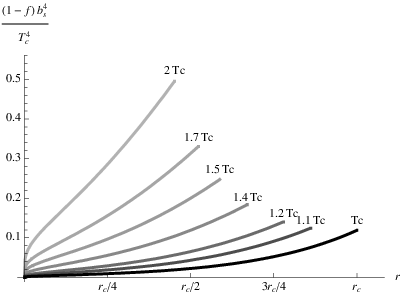
A first assessment of this relation involves determining the zeros and the region of positivity of the right-hand side. is always positive and vanishes at the horizon. For the second factor we need the asymptotics of . This factor remains positive and bounded from below in the interior and up to the horizon. It vanishes however logarithmically near the boundary as
| (97) |
This is unlike the conformal case where we obtain a constant
| (98) |
The behavior in (97) is a model artifact and is analyzed in appendix E.
Because of this, for fixed , there is a region near the boundary where becomes negative. At this stage we will avoid this region, by using a modified boundary at . We will later show that this gymnastics will be irrelevant for the computation of the jet quenching parameter, as it involves effectively the limit .
We will place the modified boundary a bit inward from the place where the factor vanishes:
| (99) |
Therefore we choose .
Then, in the range the factor is positive for sufficiently small . In this same range, vanishes only at . This is the true turning point of the string world-sheet. This is also what happens in the conformal case. It is also intuitively obvious that the relevant Wilson loop must sample also the region near the horizon.
The constant is determined by the fact that the two light-like Wilson loops are a distance apart.
| (100) |
The denominator vanishes at the turning point. The singularity is integrable1919 19 Even if we choose , the new singularity at is also integrable as suggested from (97).. Therefore, as we are interested in the small region, it is obvious from the expression above that that must also be small in the same limit.
This relation can then be expanded in powers of as
| (101) |
Therefore to leading order in
| (102) |
We are now ready to evaluate the Nambu-Goto action of the extremal configuration we have found. Starting from (94), we substitute from (96), and change integration variable from to obtain
| (103) |
As in [19, 20], we subtract from equation (103) the action of two free string straight worldsheets that hang down to the horizon. To compute this action a convenient choice of gauge is . The action of each sheet is
| (104) |
The subtracted action is therefore:
So far we have evaluated the relevant Wilson loop in the fundamental representation (by using probe quarks). On the other hand, the Wilson loop that defines the jet-quenching parameter is an adjoint one. We can obtain it in the large- limit from the fundamental using . We finally extract the jet-quenching parameter as
| (107) |
We are now ready to remove the cutoff. As the integral appearing is now well-defined up to the real boundary we may rewrite it as
| (108) |
In appendix F we obtain the small estimate of that vanishes as . We may finally write2020 20 In practise, the previous discussion including regularizing the UV is academic. The numerical calculation is done with a finite cutoff where the boundary conditions for the couplings are imposed.
| (109) |


| (direct) | (direct) | |
| 220 | - | - |
| 250 | 0.5 | 0.6 |
| 280 | 0.8 | 0.8 |
| 310 | 1.1 | 1.1 |
| 340 | 1.4 | 1.4 |
| 370 | 1.8 | 1.8 |
| 400 | 2.2 | 2.2 |
| (direct) | (energy) | (entropy) | |
| 220 | - | 0.9 | 1.0 |
| 250 | 0.5 | 1.2 | 1.3 |
| 280 | 0.8 | 1.6 | 1.7 |
| 310 | 1.1 | 2.1 | 2.2 |
| 340 | 1.4 | 2.7 | 2.8 |
| 370 | 1.8 | 3.4 | 3.4 |
| 400 | 2.2 | 4.2 | 4.2 |
| (direct) | (energy) | (entropy) | |
| 220 | - | 1.3 | 1.5 |
| 250 | 0.8 | 1.8 | 2.0 |
| 280 | 1.2 | 2.6 | 2.8 |
| 310 | 1.7 | 3.5 | 3.6 |
| 340 | 2.2 | 4.6 | 4.7 |
| 370 | 2.8 | 5.9 | 6.0 |
| 400 | 3.6 | 7.6 | 7.5 |
| (direct) | (energy) | (entropy) | |
| 220 | - | 1.0 | 1.1 |
| 250 | 0.6 | 1.4 | 1.5 |
| 280 | 0.9 | 1.9 | 2.0 |
| 310 | 1.2 | 2.5 | 2.6 |
| 340 | 1.6 | 3.2 | 3.2 |
| 370 | 2.0 | 4.0 | 4.0 |
| 400 | 2.5 | 5.0 | 4.9 |
From equation (109) we obtain, in the conformal case:
| (110) |
The conformal value, for the median value of and MeV gives GeV2/fm where we used the conversion GeV fm-1.
Numerical evaluation of equation (109) in the non-conformal IHQCD setup2121 21 In this case, the value of appearing in equation (109) is fixed as explained in Section 4. gives us a value of which is lower (at a given temperature) than the conformal value, as shown in Figures 16, 17 and 18. Tables 4 to 7 display the numerical values of the jet quenching parameter at different temperatures in the experimentally relevant range, in different temperature matching schemes.
6 Discussion and summary
In this paper we have examined several aspects associated with the physics of thermal transport phenomena in gluon plasma with potential applications to heavy ion collisions. We have used as basic model for our calculations the 5D Einstein-dilaton model with a potential proposed in [38, 39]. This is a hybrid model that incorporates features coming from string theory as well as features originating in YM, [40]. We have also used a potential, whose two phenomenological parameters have been fit to lattice YM data, [49]. This model, named Improved Holographic QCD is expected to be a very good approximation to several aspects of YM physics.
In this context we calculated the bulk viscosity by calculating the low-frequency asymptotics of the appropriate two-point function of the energy-momentum tensor. We have further calculated the drag force on a heavy quark by extending the dragging string calculation done earlier in the context of SYM, [21, 22, 23]. Finally we have calculated the jet-quenching parameter defined by the expectation value of a light-like Wilson loop, by adapting the calculation of [19, 20] from . Unlike the case of , our calculations here are numerical as no analytical solutions are known for Improved Holographic QCD with the appropriate potential. We have however derived analytically various asymptotics of the results relevant for high energy, low velocity or high temperature.
Before discussing the results, it is appropriate at this point to take a critical look and analyze potential sources of (systematic) error in our calculations.
- •
Holographic models are reliable in the context of large- expansion of the gauge theory. Therefore a priori, our results should be understood as the leading order part in the large-Nc expansion.
The issue, however, is a bit more complicated by the fact the the model we are employing is semi-phenomenological and therefore contains two phenomenological parameters (apart from the ones expected in YM) that have been fit to data in [49]. Although several lattice data are known at large-Nc, [65], others are not. In particular, the detailed thermodynamics of large-Nc YM is currently being calculated on the lattice, [66]. Therefore not all relevant input data we used have been computed at large .
In this sense the semi-phenomenological model we are using is positioned somewhere between Nc=3, YM and N YM. It is known so far that the difference in many observables in the gluon sector between these two points is of the order of 5% or less.
- •
There are no dynamical flavor degrees of freedom incorporated in the model used. In [38, 39] the incorporation of flavor branes was described at the semi-quantitative level. We have assumed that we work in the “quenched” approximation: the number of flavors which implies in particular that fermions loops are suppressed by a factor of .
The configuration of flavor branes is expected to involve a pair of space-filling and per quark flavor. These branes enter at the AdS boundary and at some point in the interior they are expected to fuse signalling chiral symmetry breaking. The configuration in the broken phase involves a space-filling brane that folds on itself and resembles closely the branes described in [67] using Boundary CFT.
The bare mass of the associated quarks enters as a source boundary condition on the relevant tachyon field, [41]. The higher the mass the stronger is the tendency on the tachyon to diverge in the IR. In the deconfined phase we expect that branes associated to light quarks cross the BH horizon and this signals the melting of the associated mesons. Branes associated to heavy quarks, will fuse outside the horizon, signaling the stability of the associated mesons. These expectations are qualitative. They have been observed in toy models, [68] but have not been yet calculated in a reliable extension of the present setup, [69].
Our estimate is that the bare quark mass is related to the flavor brane position in the following way: The energy of a string stretching from to , (the equilibrium position of string world-sheets) is equal to the bare quark mass, as detailed in section 4.5. This is expected to be asymptotically correct when the mass of the quark is much larger than the dynamical scale of the gauge theory, and we therefore do not expect a large source of error for charm and bottom quarks.
- •
There are several other sources of error, that enter between using the quantities computed here and comparing them to the eventual experimental data. Most of them have been described preciously, [19, 20, 21, 23, 33], and we do not have much more to add here. We would like however to mention one extra important aspect: deciding the appropriate temperature to be used in comparisons with data. This is an issue because in YM the deconfining transition is first order (instead of the expected cross-over in the theory with quarks) with a transition temperature that is about 50% larger than in QCD.
There is therefore a non-trivial comparison to be made. We do not know the best way to compare, but we have explored three different matchings: taking the same temperature, the same energy density or the same entropy density. Until a computation is made taking into account the fermionic degrees of freedom, this choice introduces an extra systematic error in the comparison.
This ambiguity is the same one that arises when one fixes the temperature in the holographic computations using the theory. In that case however, one must also fix the coupling constant, and this introduces an extra source of error. In our model this is not an issue, since the coupling constant runs. All observable quantities we compute are independent of the value of the coupling at a given energy, thus we do not need to fix an extra parameter by hand.
- •
There are further limitations on the range of applicability of the drag force and jet-quenching calculations, that have been discussed in the literature [70, 71]. In the drag-force calculation the velocity is limited by the position of the associated flavor brane. In a sense the world-sheet horizon should be kept away from that brane so that standard calculations of the drag force are reliable. The jet-quenching parameter seems valid in the opposite regime.
There is a further important issue concerning the physics of heavy quarks in the context of the QGP. It has been argued from various points of view,[23],[24]-[31] that the motion of a heavy quark propagating and interacting in QGP is very similar to Brownian motion. The associated description starts with a Langevin equation which contains two ingredients: a classical force (the drag force) and a fluctuation force (the “noise”) characterized by a a diffusion coefficient in the (late-time) Gaussian case.
The distribution for the kinematic data then describes a Fokker-Planck equation. In the standard non-relativistic case, the assumption of a Maxwell equilibrium solution to the Fokker-Planck equation provides a relation between the classical force and the stochastic force known in the simplest cases as the Einstein relation.
One of the relevant ingredients in the case of QGP is that the description of the Brownian motion must be relativistic. Relativistic Langevin evolutions have been described already in the relevant mathematical literature, [32]. However, in the early literature, it was assumed that the relativistic Maxwell distribution is an equilibrium solution to the Fokker-Planck equations. This leads to an Einstein-like relation that is problematic at high temperatures. This is taken as a hint that the initial assumption is false. Moreover, in the case of heavy-quark diffusion the longitudinal and transverse directions behave very differently. A recent series of papers, [28]-[31] derived the Langevin-type evolution of a heavy quark in the context of AdS/CFT by studying the small oscillations of the trailing string solution that describes the average motion of the quark. In particular, it was shown in [31] that the fluctuating force is strongly influenced by the existence of an induced 2d black-hole metric and an associated world-sheet horizon in the semiclassical trailing string solution, as detailed in section 4. In the non-relativistic limit, this world-sheet horizon and the bulk black-hole horizon coincide. The relevant diffusion coefficients are therefore computed from thermal two-point functions for the string fluctuations.
The analogous computation of such thermal correlators in our case, is more involved than the case and will be reported in a
future publication.
Below we give a summary of our results.
Bulk Viscosity:
We have computed the bulk viscosity by calculating the low frequency asymptotics of the appropriate stress tensor correlator holographically. We find that the bulk viscosity rises near the phase transition but stays always below the shear viscosity. It floats somewhat above the Buchel bound, with a coefficient of proportionality varying between 1 and 2. Therefore it is expected to affect the elliptic flow at the small percentage level [59, 13]. Knowledge of the bulk viscosity is important in extracting the shear viscosity from the data. This result is not in agreement with the lattice result near . In particular the lattice result gives a value for the viscosity that is ten times larger.
The bulk viscosity keeps increasing in the black-hole branch below the transition point until the large BH turns into the small BH at a temperature . The bulk viscosity on the small BH background is always larger than the respective one in the large BH background. In particular, we showed that the T derivative of the quantity diverges at . This is the holographic reason for the presence of a peak in near . On the other hand, as it is shown in [45], presence of (i.e. a small BH branch) is in one-to-one correspondence with color confinement at zero T. We arrive thus at the suggestion that in a (large N) gauge theory that confines color at zero T, there shall be a rise in near .
An important ingredient here was the value of the viscosity asymptotically in the small BH branch. There we correlated precisely its asymptotic value to the IR behavior of the potential. Taking also account the fact that this asymptotic value is very close to the value of the bulk viscosity near , we can derive bounds that suggest that the bulk viscosity cannot increase a lot near .
Drag Force:
The drag force we have calculated has the expected behavior. Although it increases with temperature, it does so slower than in SYM, signaling the effects of asymptotic freedom. This feature is at odds with the robustness observations for the drag force of [72].
Diffusion Time:
Based on the drag force calculation we have computed the diffusion times for a heavy external quark. The numerical values we obtain are in agreement with phenomenological models [17]. To accommodate for the fact that our models exhibits a phase transition around (i.e. about higher than in QCD), we compare our results using alternative schemes, as proposed in [33]. For example, for an external Charm quark of momentum we find (in the alternative scheme) a diffusion time of at temperature . Similarly, for a Bottom quark of the same momentum and at the same temperature we find . Generally the numbers we obtain are close to those obtained by [17] and [25].
Jet Quenching:
We have also calculated the jet quenching parameter of this model, based on the formalism of [19, 20] by computing the appropriate light-like Wilson loop. We find that grows with temperature, but slower than the growth of SYM result. Again this can be attributed to the incorporation of asymptotic freedom in our model. Using the alternative scheme to compare with experiment we find that our results are close to the lower quoted values of . For example, for a temperature of MeV, which in the alternative “energy scheme” corresponds to a temperature of MeV in our model, we find that .
However, the numbers obtained for this particular definition of jet quenching parameter seem rather low and indicate that this may not be the most appropriate definition in the holographic context. There are other ways to define , in particular using the fluctuations of the trailing string solution. This is gives a direct and more detailed input in the associated Langevin dynamics and captures the asymmetry between longitudinal and transverse fluctuations. It would be interesting to compute this, along the lines set in [28, 30, 31] and we are currently pursuing that aim.
Note added in proof
Since this paper has appeared in the archive, two papers appeared that have a direct connection to some of the issues discussed here. In reference [75] a high precision lattice calculation of the thermodynamics was performed at various . The results suggest that the thermodynamic functions vary very little with although the phase transition becomes sharper as increases. The thermodynamic functions and in particular the trace-anomaly calculated from the Improved Holographic QCD model [49] match very well the lattice data.
In reference [76] a detailed study of the hydrodymamics with a high-viscosity regime was performed. It was found that cavitation ensues for bulk or shear viscosity values a few times the PSS value, thus corroborating earlier numerical evidence, [11]. Our results indicate that cavitation (and therefore breakdown of the hydrodynamic description) is not expected to happen in the deconfined phase of the quark gluon plasma.
Acknowledgements
We would like to thank B. Bringoltz, M. Cacciari, J. Casalderrey-Solana, P. de Forcrand, R. Granier de Cassagnac, S. Gubser, U. Heinz, D. K. Hong, K. Kajantie, F. Karsch, D. Kharzeev, M. Panero, S. Pufu, F.Rocha, P. Romatchke, C. Salgado, S. J. Sin, C. Skenderis, A. Tseytlin and U. Wiedemann for discussions.
This work was partially supported by a European Union grant FP7-REGPOT-2008-1-CreteHEPCosmo-228644, an ANR grant NT05-1-41861, a CNRS PICS grant # 4172 and an ANR grant ANR-05-BLAN-0079-02.
Elias Kiritsis is on leave of absence from APC, Université Paris 7, (UMR du CNRS 7164).
APPENDIX
Appendix A The scalar variables and evaluation of the bulk viscosity
To determine we need to solve the fluctuation equation (30) numerically. This requires knowledge of the background functions , and as functions of . A very convenient reformulation of the Einstein’s equations, especially when the radial variable is taken as is explained in section 7 of [45], that we review here.
One can reduce the number of Einstein’s equations by introducing the following scalar variables:
| (111) |
where we defined . Note that and are invariant under radial coordinate transformations. These variables obey the following first order equations:
| (112) | |||||
| (113) |
As shown in [45], the thermodynamics of the dual field theory are completely determined by knowledge of and as a function of . Roughly speaking, is dual to the enthalpy and to the energy of the gluon fluid.
In solving (112) and (113) one imposes the boundary conditions at the horizon. The regularity of horizon requires
| (114) |
as . Solving (112) near the horizon determines
| (115) |
Having solved for and , one determines the metric functions and as,
| (116) | |||||
| (117) |
Now, let us compute the last metric function . The metric written in the r-frame and the -frame are:
| (118) |
Comparison determines,
| (119) |
In the formulation of the scalar variables, is given by,
| (120) |
Thus, one finds as
| (121) |
Having found the metric functions in and variables, one can rewrite the fluctuation equation (30). There are various cancellations most notably in rewriting the -dependent term in (30): The temperature T is determined by the following equation, (see equation (H.67) pf [45]) in the scalar variables:
| (122) |
Now, using the equations (113), (116), (117) and (122), the dependent term can be simplified as
With similar simplifications, the entire (30) equation can be written only in terms of and functions:
| (123) |
where
| (124) | |||||
| (125) |
To summarize: Given , one computes the functions and from (112) and (113) and the temperature from (122). Given these data, one solves (123) numerically (with the boundary conditions explained below (30)).
In passing, we note that the equation (123) can be put in a Riccati form by the change of variables : whose general solution can be found iff one knows a special solution. It is presumably possible to find a special solution for simple potentials .
Appendix B Bulk viscosity in the limit of vanishing black-hole
Here, we fill in the details of the computation that leads to equation (40). This follows from (36) in the high T limit on the small BH (). We first show that, the fluctuation coefficient goes to 1 in this limit. is given by the value of that follows from solving (123) with , and the boundary condition .
In [45], it was shown that in the limit, the functions and simplify. In particular where corresponds to the zero T solution and everywhere except . In fact, one can show that is proportional to a delta function in the limit . Thus, from (125) we observe that vanishes in this limit for all values of . In fact it also vanishes at because the term vanishes as . Therefore the fluctuation equation simplifies to
| (126) |
The solution with the aforementioned boundary condition is,
| (127) |
The integration constant is determined by the second boundary condition . On the other hand, is positive definite in the limit . This is because approaches to whereas approaches to . Hence the only way to obey the condition is to set , hence for all values of in the limit . We checked that this is indeed the case by numerical analysis.
Appendix C The adiabatic approximation in scalar variables
The approximate solution explained in [56] is given by eqs. (44) and (45). Using and (116), we observe starting from (44) that the approximation translated in scalar variables implies,
| (128) |
To verify that the second equation (45) leads to the same conclusion, we may use equation (7.38) of [45]:
| (129) |
On the other hand, [45]. Therefore, we verify that (45) also leads to (128).
We compare both sides of equation (128) in figure 19 for a large enough (so that a wider range can be compared). On this figure we also plot (the variable for the zero-T theory) for comparison.

We will now proceed to understand the approximate formula (128) independently. Suppose that is a slowly varying function of . Then, we claim that we can write
| (130) |
where is small w.r.t everywhere (this also means that is small everywhere).
Substitution of (130) in (112) gives2222 22 The proportionality constant is smooth and order one. This is firstly because everywhere, and secondly, at the point diverges, i.e. at , the boundary condition (114) guarantees that the proportionality constant is still order 1.,
| (131) |
Therefore, the condition is equivalent to is slowly varying with , namely the condition for the adiabatic approximation. This argument also shows that in the limits where becomes constant, in particular near the boundary , and near the singularity (for ), the approximation becomes exact. Figure 20 supports our arguments above by numerical evidence. Here we plot the ratio , namely the difference between the exact (numerical) result and the adiabatic approximation (normalized by the exact value) and the function . The latter provides the criterion for the validity of the adiabatic approximation. The regions where both functions become large (the region around ) coincide, as expected from our argumentation above. We also see that the approximation becomes better near the UV and the IR regions.

In passing let us also note the physics features that cannot be captured by the adiabatic approximation. The same condition, namely that varies slowly, also leads to for the zero T theory. This means vanishes in this regime. According to [45], the gluon condensate is set to zero within this approximation. Therefore, one cannot observe the phase transition at in the adiabatic approximation. By the same reasoning, we learn that the adiabatic approximation becomes worst when differs from most, i.e. when the gluon condensate is largest, in other words in the region near , see also figure 20.
Appendix D Equivalence of the axial and the gauges
According to the standard AdS/CFT dictionary the metric fluctuation is dual to in the axial gauge , whereas our computation of the bulk viscosity is carried out gauge, following [53]. In [53], it is shown that the result is independent of the gauge choice, by performing a gauge transformation between the two gauges and showing that this does not affect the coupling of the fluctuation to the corresponding operator to leading order near the boundary. In our backgrounds, this issue is slightly more subtle, due to the logarithmic corrections to the asymptotically AdS geometry.
Here we shall follow the steps in [53] and prove that indeed the gauge choice does not affect the coupling also in our backgrounds. The metric in the gauge is given in (118). Asymptotic forms of the metric functions near the boundary read (in the coordinate) ,
| (132) | |||||
| (133) | |||||
| (134) |
We want to perform a gauge transformation from the gauge I to gauge II where,
| (135) | |||||
| (136) |
Under an infinitesimal gauge transformation , the metric functions and the dilaton transform as
| (137) |
The symmetries of the problem dictate that and , .
When applied to (135) in order to get (136) these transformations reduce to the following equations. The dilaton equation yield and the 55, 50, 00 and 11 components of the second equation in (137) respectively produce [53]:
| (138) | |||
| (139) | |||
| (140) | |||
| (141) |
where prime and dot denotes derivation w.r.t. and time, respectively.
We shall assume an oscillatory form for the t-dependence of the fluctuations, and use the same symbol to denote the -dependent piece, with a slight abuse of notation. One can easily see that the following computation goes through with no change for a more general t-dependence. Using the asymptotic forms of the metric functions above, one finds an approximate solution to (138) as,
| (142) |
In order to determine the asymptotic behavior, one needs to determine near the boundary. This can be done by using the fluctuation equation for ( see [53]),
| (143) |
where is the solution to (30). Again, using the asymptotic forms of the metric functions above, one finds that the solution to (30) near boundary (with the boundary condition ) reads,
| (144) | |||||
| (145) |
where , are some integration constants. Using these in (143) one finds that for and for . Finally, substituting this in (142) gives (for ) ,
| (146) |
We see that the leading term goes as whereas the sub-leading term is suppressed as as at the boundary. Thus we can safely ignore the inhomogeneous contribution in (142) and take . Using this and the asymptotics of the metric functions above in (139) now gives,
| (147) |
Finally, using all the above, one solves (141) and (140) as (stripping off the t-dependence),
| (148) |
The operator that is dual to is ([45]) . Thus, from (146) and (148) we find that the fluctuation of the Lagrangian that is proportional to is
| (149) |
Expanding the dilatation Ward identity, to leading order in we see that, (149) vanishes. This proves that the fluctuation of the metric function couples to both in the axial gauge and in the gauge.
Appendix E UV subtleties
In a theory where the dilaton is non-trivial, there is a relevant question to be asked. In which frame is the metric asymptotically AdS? This question is void in the dual of SYM where the dilaton is trivial but not in Improved Holographic QCD where the gauge coupling is a function of the holographic coordinate. In [40] by analyzing the structure of string higher-curvature corrections, it was shown that it is consistent with the equations of motion that the string-frame metric is asymptotically AdS. This is required in order for the background solution to have the correct structure and QCD perturbation theory to emerge.
By approximating the string theory dual to QCD by a two derivative theory and a dilaton potential as it was proposed in [38, 39] this property cannot be maintained. It is not easy to see that the only option that can be implemented in the UV is an asymptotically AdS metric in the Einstein frame instead. This has as a result a few “stray logs” in several quantities that are calculated from the world-sheet action (instead of the bulk effective action). One of them is the short distance inter-quark potential calculated in [73] which is2323 23 Interestingly, it was argued in [73] that this fits better Quarkonium data than the Cornell potential. .
Other similar cases appear in this paper, in the two observables that involve the string world-sheet action. The first is the drag-force calculation. The effect of these logs appears both as the energy of the string end-point becomes asymptotically large () or when the temperature becomes large . One example is the ultra-relativistic diffusion time (82) that we reproduced here
| (150) |
The logarithmic fact is due to a factor of . Another example is the large asymptotics of the non-relativistic diffusion time in (83). It gives exactly the conformal result modulo again a factor of .
A similar effect appears in the jet-quenching calculation in section 5. Indeed, in (109), the combination vanishes logarithmically in the UV instead of asymptoting to a constant value. This occurrence perturbs the structure of the Wilson loop configuration near the boundary, but as shown there does not affect the calculation of the jet-quenching parameter.
A perturbative calculation at NLO of the diffusion time gives, [74]
| (151) |
while for large SYM it is obtained
| (152) |
Such perturbative asymptotics are not visible in the NG action.
There is however an important issue here: when and where we can trust the standard Nambu-Goto world-sheet action. The structure of the vacuum solution near the boundary, advocated in [40], suggests that since curvatures are high in that region, care is needed when using the NG action in that regime. On the other hand, the UV behavior remains qualitatively correct although in its details it may be revisable.
Appendix F The UV asymptotics of the integral (5.21)
Near in the Einstein frame, [38],
| (154) |
| (155) |
Using these relations we obtain
| (156) |
changing variables to we obtain
| (157) |
We now use
| (158) |
to finally obtain
| (159) |
valid as .
References
- [1]
J. Adams et al. [STAR Collaboration],
“Experimental and theoretical challenges in the search for the quark gluon
plasma: The STAR collaboration’s critical assessment of the evidence from
RHIC collisions,”
Nucl. Phys. A 757 (2005) 102
[ArXiv:nucl-ex/0501009];
B. B. Back et al., “The PHOBOS perspective on discoveries at RHIC,” Nucl. Phys. A 757 (2005) 28 [ArXiv:nucl-ex/0410022];
I. Arsene et al. [BRAHMS Collaboration], “Quark gluon plasma and color glass condensate at RHIC? The perspective from the BRAHMS experiment,” Nucl. Phys. A 757 (2005) 1 [ArXiv:nucl-ex/0410020];
K. Adcox et al. [PHENIX Collaboration], “Formation of dense partonic matter in relativistic nucleus nucleus collisions at RHIC: Experimental evaluation by the PHENIX collaboration,” Nucl. Phys. A 757 (2005) 184 [ArXiv:nucl-ex/0410003]. - [2] M. Luzum and P. Romatschke, “Conformal Relativistic Viscous Hydrodynamics: Applications to RHIC results at = 200 GeV,” Phys. Rev. C 78 (2008) 034915 [ArXiv:0804.4015][nucl-th].
- [3] P. Romatschke, “New Developments in Relativistic Viscous Hydrodynamics,” [ArXiv:0902.3663][hep-ph].
- [4]
G. Policastro, D. T. Son and A. O. Starinets,
“The shear viscosity of strongly coupled N = 4 supersymmetric Yang-Mills
plasma,”
Phys. Rev. Lett. 87 (2001) 081601
[ArXiv:hep-th/0104066];
P. Kovtun, D. T. Son and A. O. Starinets, “Viscosity in strongly interacting quantum field theories from black-hole physics,” Phys. Rev. Lett. 94 (2005) 111601 [arXiv:hep-th/0405231]. - [5]
E. Shuryak,
“Physics of Strongly coupled Quark-Gluon Plasma,”
[ArXiv:0807.3033][hep-ph];
D. T. Son and A. O. Starinets, “Viscosity, Black Holes, and Quantum Field Theory,” Ann. Rev. Nucl. Part. Sci. 57 (2007) 95 [ArXiv:0704.0240][hep-th]];
M. Natsuume, “String theory and quark-gluon plasma,” [ArXiv:hep-ph/0701201]. - [6]
R. Baier, P. Romatschke, D. T. Son, A. O. Starinets and M. A. Stephanov,
“Relativistic viscous hydrodynamics, conformal invariance, and holography,”
JHEP 0804 (2008) 100
[ArXiv:0712.2451][hep-th];
S. Bhattacharyya, V. E. Hubeny, S. Minwalla and M. Rangamani, “Nonlinear Fluid Dynamics from Gravity,” JHEP 0802 (2008) 045 [ArXiv:0712.2456][hep-th]. - [7] H. B. Meyer, “A calculation of the shear viscosity in SU(3) gluodynamics,” Phys. Rev. D 76 (2007) 101701 [ArXiv:0704.1801][hep-lat].
- [8] D. Kharzeev and K. Tuchin, “Bulk viscosity of QCD matter near the critical temperature,” JHEP 0809 (2008) 093 [ArXiv:0705.4280][hep-ph].
- [9] F. Karsch, D. Kharzeev and K. Tuchin, “Universal properties of bulk viscosity near the QCD phase transition,” Phys. Lett. B 663 (2008) 217 [ArXiv:0711.0914][hep-ph].
- [10]
D. Teaney,
“Finite temperature spectral densities of momentum and R-charge
correlators in N = 4 Yang Mills theory,”
Phys. Rev. D 74, 045025 (2006)
[ArXiv:hep-ph/0602044];
P. Romatschke and D. T. Son, “Spectral sum rules for the quark-gluon plasma,” [ArXiv:0903.3946][hep-ph]. - [11] H. B. Meyer, “A calculation of the bulk viscosity in SU(3) gluodynamics,” Phys. Rev. Lett. 100 (2008) 162001 [ArXiv:0710.3717][hep-lat].
- [12] G. D. Moore and O. Saremi, “Bulk viscosity and spectral functions in QCD,” JHEP 0809 (2008) 015 [ArXiv:0805.4201][hep-ph].
- [13] U. Heinz, talk at the ``The Extra Strong Quark Gluon Plasma (ESQGP)", Stony Brook, 2008
- [14] A. Adare et al. [PHENIX Collaboration], “Energy Loss and Flow of Heavy Quarks in Au+Au Collisions at = 200 GeV,” Phys. Rev. Lett. 98 (2007) 172301 [ArXiv:nucl-ex/0611018].
- [15] N. Borghini and U. A. Wiedemann, “Predictions for the LHC heavy ion programme,” J. Phys. G 35 (2008) 023001 [ArXiv:0707.0564][hep-ph].
- [16]
R. Baier, Y. L. Dokshitzer, A. H. Mueller, S. Peigne and D. Schiff,
“Radiative energy loss of high energy quarks and gluons in a finite-volume
quark-gluon plasma,”
Nucl. Phys. B 483 (1997) 291
[ArXiv:hep-ph/9607355];
“Radiative energy loss and p(T)-broadening of high energy partons in nuclei,” Nucl. Phys. B 484 (1997) 265 [ArXiv:hep-ph/9608322];
B. G. Zakharov, “Radiative energy loss of high energy quarks in finite-size nuclear matter and quark-gluon plasma,” JETP Lett. 65 (1997) 615 [ArXiv:hep-ph/9704255]. - [17] Y. Akamatsu, T. Hatsuda and T. Hirano, “Heavy Quark Diffusion with Relativistic Langevin Dynamics in the Quark-Gluon Fluid,” [ArXiv:0809.1499][hep-ph].
- [18] S. S. Gubser, S. S. Pufu, F. D. Rocha and A. Yarom, “Energy loss in a strongly coupled thermal medium and the gauge-string duality,” [ArXiv:0902.4041][hep-th].
- [19] H. Liu, K. Rajagopal and U. A. Wiedemann, “Calculating the jet quenching parameter from AdS/CFT,” Phys. Rev. Lett. 97 (2006) 182301 [ArXiv:hep-ph/0605178].
- [20] H. Liu, K. Rajagopal and U. A. Wiedemann, “Wilson loops in heavy ion collisions and their calculation in AdS/CFT,” JHEP 0703 (2007) 066; [ArXiv:hep-ph/0612168].
- [21] C. P. Herzog, A. Karch, P. Kovtun, C. Kozcaz and L. G. Yaffe, “Energy loss of a heavy quark moving through N = 4 supersymmetric Yang-Mills plasma,” JHEP 0607 (2006) 013; [ArXiv:hep-th/0605158].
- [22] S. S. Gubser, “Drag force in AdS/CFT,” Phys. Rev. D 74 (2006) 126005 [ArXiv:hep-th/0605182].
- [23] J. Casalderrey-Solana and D. Teaney, “Heavy quark diffusion in strongly coupled N = 4 Yang Mills,” Phys. Rev. D 74 (2006) 085012 [ArXiv:hep-ph/0605199].
- [24] B. Svetitsky, “Diffusion of Charmed Quark in the Quark Gluon PLasma,” Phys. Rev. D 37 (1988) 2484.
- [25] H. van Hees and R. Rapp, “Thermalization of Heavy Quarks in the Quark-Gluon Plasma,” Phys. Rev. C 71 (2005) 034907 [ArXiv:nucl-th/0412015].
- [26] G. D. Moore and D. Teaney, “How much do heavy quarks thermalize in a heavy ion collision?,” Phys. Rev. C 71 (2005) 064904 [ArXiv:hep-ph/0412346].
- [27] H. van Hees, V. Greco and R. Rapp, “Heavy-quark probes of the quark-gluon plasma at RHIC,” Phys. Rev. C 73 (2006) 034913 [ArXiv:nucl-th/0508055].
- [28] S. S. Gubser, “Momentum fluctuations of heavy quarks in the gauge-string duality,” Nucl. Phys. B 790 (2008) 175 [ArXiv:hep-th/0612143].
- [29] J. de Boer, V. E. Hubeny, M. Rangamani and M. Shigemori, “Brownian motion in AdS/CFT,” [ArXiv:0812.5112][hep-th].
- [30] D. T. Son and D. Teaney, “Thermal Noise and Stochastic Strings in AdS/CFT,” [ArXiv:0901.2338][hep-th].
- [31] G. C. Giecold, E. Iancu and A. H. Mueller, “Stochastic trailing string and Langevin dynamics from AdS/CFT,” [ArXiv:0903.1840][hep-th].
- [32]
F. Debbasch, K. Mallick and K. P. Rivet, J. of Stat. Phys., 88 (1997) 945.
C. Chevalier and F. Debbasch, J. Math. Phys. 49 (2008) 043303. - [33] S. S. Gubser, “Comparing the drag force on heavy quarks in N = 4 super-Yang-Mills theory and QCD,” Phys. Rev. D 76 (2007) 126003 [ArXiv:hep-th/0611272].
- [34] S. Caron-Huot, P. Kovtun, G. D. Moore, A. Starinets and L. G. Yaffe, “Photon and dilepton production in supersymmetric Yang-Mills plasma,” JHEP 0612 (2006) 015 [ArXiv:hep-th/0607237].
- [35]
S. J. Sin and I. Zahed,
“Holography of radiation and jet quenching,”
Phys. Lett. B 608 (2005) 265
[ArXiv:hep-th/0407215];
“Ampere’s Law and Energy Loss in AdS/CFT Duality,” Phys. Lett. B 648 (2007) 318 [ArXiv:hep-ph/0606049]. - [36]
J. Erlich, E. Katz, D. T. Son and M. A. Stephanov,
“QCD and a holographic model of hadrons,”
Phys. Rev. Lett. 95, 261602 (2005)
[arXiv:hep-ph/0501128];
L. Da Rold and A. Pomarol, “Chiral symmetry breaking from five dimensional spaces,” Nucl. Phys. B 721, 79 (2005) [ArXiv:hep-ph/0501218]. - [37] A. Karch, E. Katz, D. T. Son and M. A. Stephanov, “Linear confinement and AdS/QCD,” Phys. Rev. D 74 (2006) 015005 [ArXiv:hep-ph/0602229].
- [38] U. Gursoy and E. Kiritsis, “Exploring improved holographic theories for QCD: Part I,” JHEP 0802 (2008) 032 [ArXiv:0707.1324 ][hep-th].
- [39] U. Gursoy, E. Kiritsis and F. Nitti, “Exploring improved holographic theories for QCD: Part II,” JHEP 0802 (2008) 019 [ArXiv:0707.1349] [hep-th].
- [40] E. Kiritsis, “Dissecting the string theory dual of QCD,” [ArXiv:0901.1772][hep-th].
- [41] R. Casero, E. Kiritsis and A. Paredes, “Chiral symmetry breaking as open string tachyon condensation,” Nucl. Phys. B 787 (2007) 98; [ArXiv:hep-th/0702155].
- [42] F. Bigazzi, R. Casero, A. L. Cotrone, E. Kiritsis and A. Paredes, “Non-critical holography and four-dimensional CFT’s with fundamentals,” JHEP 0510 (2005) 012 [ArXiv:hep-th/0505140].
- [43] G. Bertoldi, F. Bigazzi, A. L. Cotrone and J. D. Edelstein, “Holography and Unquenched Quark-Gluon Plasmas,” Phys. Rev. D 76 (2007) 065007 [ArXiv:hep-th/0702225].
- [44] U. Gursoy, E. Kiritsis, L. Mazzanti and F. Nitti, “Deconfinement and Gluon Plasma Dynamics in Improved Holographic QCD, Phys. Rev. Lett. 101, 181601 (2008) [ArXiv:0804.0899][hep-th].
- [45] U. Gursoy, E. Kiritsis, L. Mazzanti and F. Nitti, “Holography and Thermodynamics of 5D Dilaton-gravity, JHEP 0905, 033 (2009) [ArXiv:0812.0792 ][hep-th].
- [46] S. S. Gubser and A. Nellore, “Mimicking the QCD equation of state with a dual black hole,” Phys. Rev. D 78, 086007 (2008) [ArXiv:0804.0434] [hep-th].
- [47] O. DeWolfe and C. Rosen, “Robustness of Sound Speed and Jet Quenching for Gauge/Gravity Models of Hot QCD,” JHEP 0907, 022 (2009) [ArXiv:0903.1458][hep-th].
- [48] E. Vicari and H. Panagopoulos, “Theta dependence of SU(N) gauge theories in the presence of a topological term,”Phys. Rept. 470, 93 (2009) [ArXiv:0803.1593][hep-th].
- [49] U. Gursoy, E. Kiritsis, L. Mazzanti and F. Nitti, “Improved Holographic QCD at finite Temperature: comparison with data, Nucl. Phys. B 820, 148 (2009) [ArXiv:0903.2859][hep-th].
- [50] Y. Kinar, E. Schreiber and J. Sonnenschein, “Q anti-Q potential from strings in curved spacetime: Classical results,” Nucl. Phys. B 566, 103 (2000) [ArXiv:hep-th/9811192].
- [51] G. Policastro, D. T. Son and A. O. Starinets, “The shear viscosity of strongly coupled N = 4 supersymmetric Yang-Mills plasma,” Phys. Rev. Lett. 87 (2001) 081601 [ArXiv:hep-th/0104066].
- [52] T. Springer, “Sound Mode Hydrodynamics from Bulk Scalar Fields,” Phys. Rev. D 79, 046003 (2009) [[ArXiv:arXiv:0810.4354][hep-th]].
- [53] S. S. Gubser, S. S. Pufu and F. D. Rocha, “Bulk viscosity of strongly coupled plasmas with holographic duals,” JHEP 0808 (2008) 085 [ArXiv:0806.0407][hep-th].
- [54] P. Arnold, C. Dogan and G. D. Moore, “The bulk viscosity of high-temperature QCD,” Phys. Rev. D 74 (2006) 085021 [arXiv:hep-ph/0608012].
- [55] H. A. Chamblin and H. S. Reall, “Dynamic dilatonic domain walls,” Nucl. Phys. B 562 (1999) 133 [arXiv:hep-th/9903225].
- [56] S. S. Gubser and A. Nellore, “Mimicking the QCD equation of state with a dual black hole,” Phys. Rev. D 78 (2008) 086007 [arXiv:0804.0434 [hep-th]].
- [57] A. Buchel, “Bulk viscosity of gauge theory plasma at strong coupling,” Phys. Lett. B 663 (2008) 286 [ArXiv:0708.3459][hep-th].
- [58] I. Kanitscheider and K. Skenderis, “Universal hydrodynamics of non-conformal branes,” JHEP 0904 (2009) 062 [ArXiv:0901.1487][hep-th].
- [59] H. Song and U. W. Heinz, “Extracting the QGP viscosity from RHIC data – a status report from viscous hydrodynamics,” [ArXiv:0812.4274][nucl-th].
- [60] A. E. Lawrence and E. J. Martinec, “Black Hole Evaporation Along Macroscopic Strings,” Phys. Rev. D 50 (1994) 2680 [ArXiv:hep-th/9312127].
- [61] Y. Chen et al., “Glueball spectrum and matrix elements on anisotropic lattices,” Phys. Rev. D 73, 014516 (2006) [ArXiv:hep-lat/0510074].
- [62] G. Beuf, C. Marquet and B. W. Xiao, “Heavy-quark energy loss and thermalization in a strongly coupled SYM plasma, [ArXiv:0812.1051][hep-ph].
- [63] S. Datta, F. Karsch, P. Petreczky and I. Wetzorke, “Behavior of charmonium systems after deconfinement,” Phys. Rev. D 69, 094507 (2004); [ArXiv:hep-lat/0312037].
- [64] M. Luzum and P. Romatschke, “Viscous Hydrodynamic Predictions for Nuclear Collisions at the LHC,” [ArXiv:arXiv:0901.4588][nucl-th].
- [65]
B. Lucini, M. Teper and U. Wenger,
“The deconfinement transition in SU(N) gauge theories,”
Phys. Lett. B 545 (2002) 197
[ArXiv:hep-lat/0206029];
“The high temperature phase transition in SU(N) gauge theories,” JHEP 0401 (2004) 061 [ArXiv:hep-lat/0307017];
“Properties of the deconfining phase transition in SU(N) gauge theories,” JHEP 0502, 033 (2005) [ArXiv:hep-lat/0502003];
B. Lucini and M. Teper, “SU(N) gauge theories in four dimensions: Exploring the approach to N =,” JHEP 0106, 050 (2001) [ArXiv:hep-lat/0103027]. - [66] M. Panero, private communication.
- [67]
A. Fotopoulos, V. Niarchos and N. Prezas,
“D-branes and extended characters in SL(2,R)/U(1),”
Nucl. Phys. B 710 (2005) 309
[ArXiv:hep-th/0406017];
“D-branes and SQCD in non-critical superstring theory,” JHEP 0510 (2005) 081 [ArXiv:hep-th/0504010]. - [68] J. Erdmenger, N. Evans, I. Kirsch and E. Threlfall, “Mesons in Gauge/Gravity Duals - A Review,” Eur. Phys. J. A 35 (2008) 81 [ArXiv:0711.4467][hep-th].
- [69] U. Gursoy, E. Kiritsis, L. Mazzanti, F. Nitti, A. Paredes, work in progress.
- [70] J. Casalderrey-Solana and D. Teaney, “Transverse momentum broadening of a fast quark in a N = 4 Yang Mills plasma,” JHEP 0704 (2007) 039 [ArXiv:hep-th/0701123].
- [71] K. B. Fadafan, H. Liu, K. Rajagopal and U. A. Wiedemann, “Stirring Strongly Coupled Plasma,” Eur. Phys. J. C 61 (2009) 553 [ArXiv:0809.2869][hep-ph].
- [72] H. Liu, K. Rajagopal and Y. Shi, “Robustness and Infrared Sensitivity of Various Observables in the Application of AdS/CFT to Heavy Ion Collisions,” JHEP 0808 (2008) 048 [ArXiv:0803.3214][hep-ph].
- [73] D. f. Zeng, “Heavy quark potentials in some renormalization group revised AdS/QCD models,” Phys. Rev. D 78 (2008) 126006 [ArXiv:0805.2733][hep-th].
- [74]
S. Caron-Huot and G. D. Moore,
“Heavy quark diffusion in perturbative QCD at next-to-leading order,”
Phys. Rev. Lett. 100 (2008) 052301
[ArXiv:0708.4232][hep-ph];
“Heavy quark diffusion in QCD and N=4 SYM at next-to-leading order,” JHEP 0802 (2008) 081 [ArXiv:0801.2173][hep-ph]. - [75] M. Panero, “Thermodynamics of the QCD plasma and the large-N limit,” [ArXiv:0907.3719][hep-lat].
- [76] K. Rajagopal and N. Tripuraneni, “Bulk Viscosity and Cavitation in Boost-Invariant Hydrodynamic Expansion,” [ArXiv:0908.1785][hep-ph].