Random quantum channels II: Entanglement of random subspaces, Rényi entropy estimates and additivity problems

A non-commutative probability space is an algebra $\mathcal{A}$ with unit endowed with a tracial state $\varphi$. An element of $\mathcal{A}$ is called a (non-commutative) random variable. In this paper we shall be mostly concerned with the non-commutative probability space of random matrices $(\mathcal{M}_{n}(L^{\infty-}(\Omega,\mathbb{P})),\mathbb{E}[n^{-1}\trace(\cdot)])$ (we use the standard notation $L^{\infty-}(\Omega,\mathbb{P})=\cap_{p\geqslant 1}L^{p}(\Omega,\mathbb{P})$).

Let $\mathcal{A}_{1},\ldots,\mathcal{A}_{k}$ be subalgebras of $\mathcal{A}$ having the same unit as $\mathcal{A}$. They are said to be free if for all $a_{i}\in\mathcal{A}_{j_{i}}$ ($i=1,\ldots,k$) such that $\varphi(a_{i})=0$, one has

as soon as $j_{1}\neq j_{2}$, $j_{2}\neq j_{3},\ldots,j_{k-1}\neq j_{k}$. Collections $S_{1},S_{2},\ldots$ of random variables are said to be free if the unital subalgebras they generate are free.

Let $(a_{1},\ldots,a_{k})$ be a $k$-tuple of selfadjoint random variables and let $\mathbb{C}\langle X_{1},\ldots,X_{k}\rangle$ be the free $*$-algebra of non commutative polynomials on $\mathbb{C}$ generated by the $k$ indeterminates $X_{1},\ldots,X_{k}$. The joint distribution of the family $\{a_{i}\}_{i=1}^{k}$ is the linear form

Given a $k$-tuple $(a_{1},\ldots,a_{k})$ of free random variables such that the distribution of $a_{i}$ is $\mu_{a_{i}}$, the joint distribution $\mu_{(a_{1},\ldots,a_{k})}$ is uniquely determined by the $\mu_{a_{i}}$’s. A family $(a_{1}^{n},\ldots,a_{k}^{n})_{n}$ of $k$-tuples of random variables is said to converge in distribution towards $(a_{1},\ldots,a_{k})$ iff for all $P\in\mathbb{C}\langle X_{1},\ldots,X_{k}\rangle$, $\mu_{(a_{1}^{n},\ldots,a_{k}^{n})}(P)$ converges towards $\mu_{(a_{1},\ldots,a_{k})}(P)$ as $n\to\infty$. Sequences of random variables $(a_{1}^{n})_{n},\ldots,(a_{k}^{n})_{n}$ are called asymptotically free as $n\to\infty$ iff the $k$-tuple $(a_{1}^{n},\ldots,a_{k}^{n})_{n}$ converges in distribution towards a family of free random variables.

The following result was contained in [22] (see also [9]).

Let us fix real numbers $0\leqslant\alpha,\beta\leqslant 1$, and consider, for all $n$, a selfadjoint projector $\pi_{n}\in\mathcal{M}_{n}(\mathbb{C})$ of rank $q_{n}$ such that asymptotically $q_{n}\sim\alpha n$ as $n\to\infty$. Let $\pi_{n}^{\prime}$ be a projector of rank $q_{n}^{\prime}$ such that $q_{n}^{\prime}\sim\beta n$, and assume that it can be written under the form $U\pi_{n}U^{*}$, where $U$ is a Haar distributed unitary random matrix independent from $\pi_{n}$

It is a consequence of Theorem 2.1, that $\pi_{n}$ and $\pi_{n}^{\prime}$ are asymptotically free. Therefore $\pi_{n}\pi_{n}^{\prime}\pi_{n}$ has an empirical eigenvalues distribution converging towards a probability measure. This measure is usually denoted by $\mu_{1}\boxtimes\mu_{2}$, where $\mu_{1},\mu_{2}$ are the limit empirical eigenvalue distributions of the projectors $\pi_{n}$ and $\pi^{\prime}_{n}$ respectively:

In this specific case, we can compute explicitly $\mu_{1}\boxtimes\mu_{2}$. For this purpose, we introduce two 2-variable functions which will be of great importance in what follows.

Let us omit the variables of $\varphi^{+/-}$ and rewrite

It follows then from [23], Example 3.6.7, that

The proof relies on a technique introduced by Voiculescu to compute $\mu_{1}\boxtimes\mu_{2}$ in general, called the $S$-transform. For more details, we refer the interested reader to [23]. Since we are only interested in $\varphi^{+}$, we consider the two-variable function $\varphi:[0,1]^{2}\to[0,1]$

In the case where $\alpha+\beta<1$, the ranges of $\pi_{n}$ and $\pi^{\prime}_{n}$ do not (generically) overlap and $\varphi(\alpha,\beta)<1$. The previous asymptotic freeness results imply that almost surely,

We are interested in whether we actually have

This turns out to be true. This is an involved result whose proof we won’t discuss here. We just recall the result below as a theorem, following [7] (Theorem 4.15), see also [19].

Let $\Delta_{k}=\{x\in\mathbb{R}_{+}^{k}\,|\,\sum_{i=1}^{k}x_{i}=1\}$ be the $(k-1)$-dimensional probability simplex. For a positive real number $p>0$, define the Rényi entropy of order $p$ of a probability vector $x\in\Delta_{k}$ to be

Since $\lim_{p\to 1}H^{p}(x)$ exists, we define the Shannon entropy of $x$ to be this limit, namely:

We extend these definitions to density matrices by functional calculus:

Given a vector $x\in\mathbb{C}^{n},\left\|x\right\|=1$, we call $P_{x}$ the rank one orthogonal projection onto the span of $x$. Using Dirac’s bra-ket notation, $P_{x}=|x\rangle\langle x|$. More generally, for a subspace $V\subset\mathbb{C}^{n}$, we denote by $P_{V}$ the orthogonal projection onto $V$ in $\mathcal{M}_{n}(\mathbb{C})$.

A quantum channel is a linear completely positive trace preserving map $\Phi:\mathcal{M}_{n}(\mathbb{C})\to\mathcal{M}_{k}(\mathbb{C})$. The trace preservation condition means that density matrices are mapped to density matrices, and the complete positivity reads:

We recall that according to Stinespring theorem, a linear map $\Phi:\mathcal{M}_{n}(\mathbb{C})\to\mathcal{M}_{k}(\mathbb{C})$ is a quantum channel if and only if there exists a finite dimensional Hilbert space $\mathcal{K}=\mathbb{C}^{d}$, and a partial isometry $V\in\End(\mathbb{C}^{n},\mathbb{C}^{kd})$ (satisfying $V^{*}V=\I_{n}$) such that

For a quantum channel $\Phi:\mathcal{M}_{n}(\mathbb{C})\to\mathcal{M}_{k}(\mathbb{C})$, we define its minimum output Rényi entropy (of order $p$) by

Since the Rényi entropies are concave functions, their minima are attained on the extremal points of the set of density matrices and hence

We fix an integer $k$ and a real number $t\in(0,1)$. For each $n$, let $U_{n}\in\mathcal{M}_{nk}(\mathbb{C})$ be a random unitary matrix distributed according to the Haar measure, and $q_{n}$ be a projection of $\mathcal{M}_{nk}(\mathbb{C})$ of trace $p_{n}$ such that $p_{n}/(kn)\sim t$ as $n\to\infty$. To $q_{n}$ we associate a non-unital matrix algebra map $\chi_{n}:\mathcal{M}_{p_{n}}(\mathbb{C})\to\mathcal{M}_{nk}(\mathbb{C})$ satisfying $\chi_{n}(1)=q_{n}$. The choice of $\chi_{n}$ is unique up to unitary conjugation, and the actual choice of $\chi_{n}$ is irrelevant for the computations we want to perform - in the sense that any choice will yield the same results.

We study the sequence of random channels

given by

Graphically, our model amounts to Figure 1. We refer to the first paper of this series, [8] for details about this graphical notation.

We are interested in the random process given by the set of all possible eigenvalues of $\Phi(X)$ as $n\to\infty$. In our setup, we deal with $k$ eigenvalues.

Let $V_{n}$ be the image of $U\chi_{n}U^{*}$. This is a random vector space in $\mathbb{C}^{n}\otimes\mathbb{C}^{k}$ of dimension $p_{n}$ distributed according to the uniform measure on the Grassmannian space $\Gr_{p_{n}}(\mathbb{C}^{nk})$.

If we can ensure that the entanglement of every norm one vector $x\in V_{n}$ in $\mathbb{C}^{n}\otimes\mathbb{C}^{k}$ is large with high probability for the uniform measure on $V_{n}\in\Gr_{p_{n}}(\mathbb{C}^{nk})$, this will yield new entropy bounds. The entanglement is always a concave function of the principal values of $x$. We recall that for an element $x\in\mathbb{C}^{n}\otimes\mathbb{C}^{k}$ we denote $\lambda(x)$ and $\rk(x)$ the singular values and the rank of $x$, when viewed as a matrix $x\in\mathcal{M}_{n\times k}(\mathbb{C})$. In quantum information theory, these quantities are also called the Schmidt coefficients and the Schmidt rank of $x$ respectively:

where $\{e_{i}\}$ and $\{f_{i}\}$ are orthonormal families from $\mathbb{C}^{n}$ and $\mathbb{C}^{k}$ respectively. Both quantities can also be expressed as the rank and respectively the spectrum of the reduced density matrix $\trace_{n}P_{x}$. The strategy adopted in this paper is to describe a convex polyhedron such that with high probability, for a vector subspace $V$ chosen at random, for all input $x\in V$, the eigenvalue vector $\lambda(x)$ belongs to a neighborhood of this convex set.

Some results are already available in order to quantify the entanglement of generic spaces in $\Gr_{p_{n}}(\mathbb{C}^{n}\otimes\mathbb{C}^{k})$. The best result known so far is arguably the following theorem of Hayden, Leung and Winter in [15]:

To prove this result, the authors require sophisticated methods from asymptotic geometry theory. In particular, they need estimates on the covering numbers of unitary groups by balls of radius $\varepsilon$ and results of concentration of measure. The results of concentration of measure are applied to a specific measure of entanglement (e.g. one entropy $H^{p}$), therefore the measure of entanglement does not deal directly with the behavior of the Schmidt coefficients, but rather with the behavior of a function of them.

Our strategy is to describe a convex polyhedron $K$ inside the probability simplex $\Delta_{k}$ with the property that, for all $\varepsilon>0$, almost surely when $n$ goes to infinity, all input density matrices $\rho\geqslant 0,\trace(\rho)=1$, are mapped to output states $\Phi(\rho)$ whose spectra are contained $K+\varepsilon$, the $\varepsilon$-neighborhood of $K$.

For $t\in(0,1)$, let us first define the vector $\beta^{(t)}\in\mathbb{R}^{k}$, where

One can check directly that $\beta^{(t)}$ is a probability vector and that it is a non-increasing sequence. Moreover, $\beta^{(t)}_{1}=\varphi(1/k,t)$ and $\beta^{(t)}_{j}=0$ for $j\geqslant\lfloor k(1-t)\rfloor+2$.

Since the majorization partial order plays an important role in this situation, let us remind here the definition and some basic properties of this relation. For two probability vectors $x,y\in\Delta_{k}$, we say that $x$ is majorized by $y$ (and we write $x\prec y$) iff for all $j\in\{1,\ldots,k\}$

where $x^{\downarrow}$ and $y^{\downarrow}$ are the decreasing rearrangements of $x$ and $y$; note that for $j=k$ we actually have an equality, since $x$ and $y$ are probability vectors. We extend the functions $s_{j}$, by functional calculus, to selfadjoint matrices $X\in\mathcal{M}_{k}(\mathbb{C})$. The majorization relation can also be characterized in the following way: for a probability vector $y$ and a permutation $\sigma\in\mathfrak{S}_{k}$, denote by $\sigma.y$ the vector obtained by permuting the coordinates of $y$ along $\sigma$ : $(\sigma.y)_{i}=y_{\sigma(i)}$. Then

where $S(y)$ is the convex hull of the set $\{\sigma.y\,|\,\sigma\in\mathfrak{S}_{k}\}$. Moreover, the extremal points of $S(y)$ are exactly $y$ and its permutations $\sigma.y$. In Figure 2, we plot $\Delta_{3}$, the 2-dimensional simplex together with the sets $S(\beta^{(t)})$, for $t=1/k^{\prime}$ and $k^{\prime}=2,3,4,5,10,20,50,100$. Notice that for $k^{\prime}=2,3$, the set $S(\beta^{(1/k^{\prime})})$ touches the triangle $\Delta_{3}$, because of the fact that $\beta^{(t)}$ has in this case a zero coordinate.

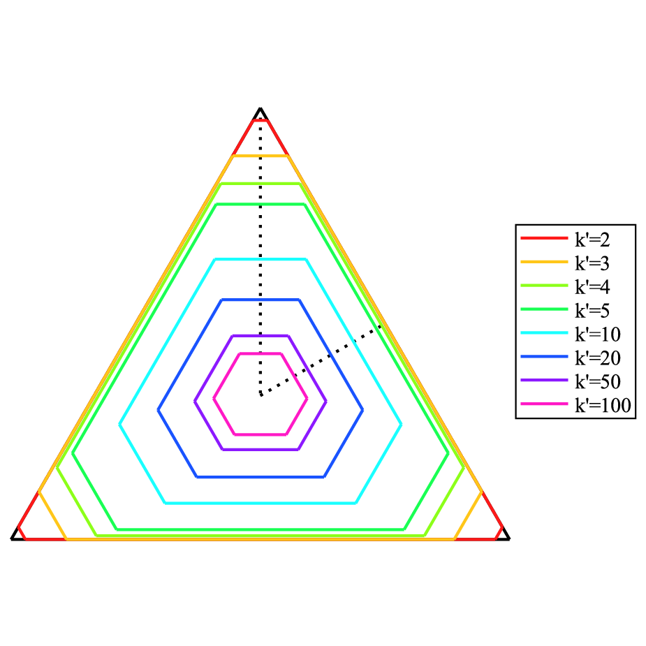
We can now state the main result of this section:

We split the proof of Theorem 4.1 into several lemmas. The first one is an easy consequence of the definition of the operator norm.

The following lemma is a reformulation of the min-max theorem:

We are interested in majorization inequalities which hold uniformly for all norm one elements of a subspace $V$. In other words, we are interested in the quantity

Since $k$ is a fixed parameter of our model, in order to compute the maximum over the Grassmannian, it suffices to consider only a finite number of subspaces $F$:

Note that in Lemma 4.4, $N$ does depend on $\varepsilon$ but can be chosen to be finite for any $\varepsilon>0$.

Now we are ready to prove Theorem 4.1.

The interest of Theorem 4.1 in comparison to Theorem 3.2 is that it does not rely specifically on one measurement of entanglement, as we are able to confine almost surely the eigenvalues in a convex set. Also, our argument relies neither on concentration inequalities nor on net estimates, as we fix $k$. However, unlike Theorem 3.2, Theorem 4.1 does not give explicit control on $n$. It is theoretically possible to give an explicit control on $n$ (using techniques introduced in [19]), but this would lead to considerably involved technicalities.

Once the eigenvalues of the output of a channel have been confined inside a fixed convex polyhedron, entropy inequalities follow easily. Indeed, the confining polyhedron is defined in terms of the majorization partial order, and thus the notion of Schur-convexity (see [4]) is crucial in what follows.

A function $f:\mathbb{R}^{k}\to\mathbb{R}$ is said to be Schur-convex if $x\prec y$ implies $f(x)\leqslant f(y)$. The Rényi entropies $H^{p}$ are Schur-concave, and thus majorization relations $x\prec y$ imply $H^{p}(x)\geqslant H^{p}(y)$ for all $p\geqslant 1$. The reciprocal implication has been studied in [1, 2]: entropy inequalities $H^{p}(x)\geqslant H^{p}(y)$ (for all $p\geqslant 1$) characterize a weaker form of majorization called catalytic majorization, which has applications in LOCC protocols for the transformation of bipartite states.

For the purposes of this paper, the main corollary of Theorem 4.1 is the following

We start with a crucial recent series of result, which we summarize into the following theorem:

This theorem results mainly from the papers [12, 14, 16]. Note that the equality

for any $\Phi_{1}$ and $\Phi_{2}$ and any $p>1$ was a conjecture until 2007, and that even nowadays, no concrete counterexamples are known for $p$ small or $p=1$.

In order to provide counterexamples for the additivity conjectures, one has to produce lower bounds for the minimum output entropy of single copies of the channels (and this is where Theorem 4.1 is useful) and upper bounds for the minimum output entropy of the tensor product of the quantum channels. The latter task is somewhat easier, since one has to exhibit a particular input state such that the output has low entropy.

The choice of the input state for the product channel is guided by the following observation. It is clear that if one chooses a product input state $\rho=\rho_{1}\otimes\rho_{2}$, then the output state is still in product form, and the entropies add up:

Hence, such choices cannot violate the additivity of Rényi entropies. Instead, one has to look at entangled states, and the maximally entangled states are obvious candidates.

All our examples rely on the study of the product of conjugate channels

where

have been introduced in subsection 3.2. Our task is to obtain a good upper bound for

Our strategy is systematically to write

where $E_{tnk}$ is the maximally entangled state over the input space $(\mathbb{C}^{tnk})^{\otimes 2}$. More precisely, $E_{tnk}$ is the projection on the Bell vector

where $\{e_{i}\}_{i=1}^{tnk}$ is a fixed basis of $\mathbb{C}^{tnk}$. Using the graphical formalism of [8], we are dealing with the diagram in Figure 3 (recall that square symbols correspond to $\mathbb{C}^{k}$, round symbols correspond to $\mathbb{C}^{n}$, diamond ones to $\mathbb{C}^{tnk}$ and triangle-shaped symbols correspond to $\mathbb{C}^{1/t}$).

The random matrix $\Phi_{n}\otimes\overline{\Phi}_{n}(E_{tnk})$ was thoroughly studied in our previous paper [8] and we recall here one of the main results of this paper:

From this we deduce the following corollary, which gives an upper bound for the minimum output entropy for the product channel $\Phi\otimes\overline{\Phi}$:

In this section, we start by fixing $t=1/2$. We assume that $k$ is even, in order to avoid non-integer dimensions. A value of $1/2$ for $t$ means that the environment to which the input of the channel is coupled is 2-dimensional, i.e. a single qubit. The main result of this section is that we obtain a violation of the Rényi entropy in this simplest purely quantum case, $k^{\prime}=2$.

Using Theorem 5.2, the asymptotic eigenvalue vector for the output of the product channel is

References

- [1] Aubrun, G. and Nechita, I. Catalytic majorization and norms. Comm. Math. Phys. 278 (2008), no. 1, 133–144.
- [2] Aubrun, G. and Nechita, I. Stochastic domination for iterated convolutions and catalytic majorization. To appear in Ann. Inst. H. Poincaré Probab. Statist.
- [3] Bengtsson, I., Życzkowski, K. Geometry of quantum states. An introduction to quantum entanglement. Cambridge University Press, Cambridge, 2006. xii+466 pp.
- [4] R. Bhatia, Matrix Analysis. Graduate Texts in Mathematics, 169. Springer-Verlag, New York, 1997.
- [5] Brandao, F., Horodecki, M. S. L. On Hastings’s counterexamples to the minimum output entropy additivity conjecture. arXiv/0907.3210v1.
- [6] Braunstein, S. L. Geometry of quantum inference. Phys. Lett. A 219 (1996), no. 3-4, 169–174.
- [7] Collins, B. Product of random projections, Jacobi ensembles and universality problems arising from free probability Probab. Theory Related Fields, 133(3):315�344, 2005.
- [8] Collins, B. and Nechita, I. Random quantum channels I: Graphical calculus and the Bell state phenomenon. To appear in Comm. Math. Phys.
- [9] Collins, B. and Śniady, P. Integration with respect to the Haar measure on unitary, orthogonal and symplectic group. Comm. Math. Phys. 264 (2006), no. 3, 773–795.
- [10] M. Fukuda, C. King Entanglement of random subspaces via the Hastings bound arXiv:0907.5446
- [11] Haagerup, U. and Thorbjørnsen, S. A new application of random matrices: is not a group. Ann. of Math. (2) 162 (2005), no. 2, 711–775.
- [12] Hastings, M.B. A Counterexample to Additivity of Minimum Output Entropy arXiv/0809.3972v3, Nature Physics 5, 255 (2009)
- [13] Hayashi, M. Quantum information. An introduction. Springer-Verlag, Berlin, 2006.
- [14] Hayden, P. The maximal p-norm multiplicativity conjecture is false arXiv/0707.3291v1
- [15] Hayden, P., Leung, D. and Winter A. Aspects of generic entanglement Comm. Math. Phys. 265 (2006), 95–117.
- [16] Hayden, P. and Winter A. Counterexamples to the maximal p-norm multiplicativity conjecture for all . Comm. Math. Phys. 284 (2008), no. 1, 263–280.
- [17] Werner R. and Hoelvo, A. Counterexample to an additivity conjecture for output purity of quantum channels. Journal of Mathematical Physics 43, 4353–4357, 2002.
- [18] Fukuda M., King C. and Moser A. Comments on HastingsÕ Additivity Counterexamples. arXiv/0905.3697v1
- [19] Ledoux, M. Differential operators and spectral distributions of invariant ensembles from the classical orthogonal polynomials part I: the continuous case. Elect. Journal in Probability 9, 177–208 (2004)
- [20] Nechita, I. Asymptotics of random density matrices. Ann. Henri Poincaré 8 (2007), no. 8, 1521–1538.
- [21] Nica, A and Speicher, R. Lectures on the combinatorics of free probability, volume 335 of London Mathematical Society Lecture Note Series. Cambridge University Press, Cambridge, 2006.
- [22] Voiculescu, D.V. A strengthened asymptotic freeness result for ran- dom matrices with applications to free entropy Internat. Math. Res. Notices, (1):41�63, 1998.
- [23] Voiculescu, D.V., Dykema. K.J. and Nica, A. Free random variables, AMS (1992).
- [24] Życzkowski, K., Sommers, H.-J. Induced measures in the space of mixed quantum states. J. Phys. A 34 (2001), no. 35, 7111–7125.