Quantum phase transition of the one-dimensional transverse field compass model

The quantum compass model has been studied extensively in recent years due to the possible long range orbital order and the quantum phase transitions (QPTs)[1, 2, 3, 4, 5, 6, 7, 8]. First, the model could be used to describe the Mott insulators with orbit degeneracies. It depends on the lattice geometry, and belongs to the low energy Hamiltonian originated from the magnetic interactions in Mott-Hubbard systems with the strong spin-orbit coupling[9, 10]. For simplicity, the 1D quantum compass model is regarded as the coupling along one of bonds which shows an Ising type, but different spin components are active along other bond directions. It is exactly the same as the 1D reduced Kitave model[11, 12, 13, 14]. The symmetry of the pseudo-spin Hamiltonian is much lower than SU(2). It is shown in the numerical results that the eigenstates are at least twofold degenerate or highly degenerate[1, 5]. Recently, because of degeneracy in the ground-state (GS), the protected qubit can be implemented, a scalable and error-free scheme of the quantum computation can be designed in this simple model[3].

To shed some insights into this model, a exact solution is clearly desirable. By applying Jordan and Wigner transformation to the pseudo-spin operators, Brzezicki et al. were able to map it into a spinless fermion model and determine the spectrum exactly[5]. More recently, the exact solution of 1D period-two compass model has also been obtained by the present authors and a collaborator with a slightly different method[7]. In order to be useful for quantum information, the GS must be protected from local perturbations, but the spectrum for $h=0$ is gapless in the thermodynamic limit. The extension to finite fields is a crucial step in the search for systems supporting naturally robust quantum information[15]. To the best of our knowledge, the 1D compass model in the transverse magnetic field has not been studied so far, which may be also of fundamental significance. The symmetry of the system is further broken when the transverse magnetic field is applied. The behavior of the energy gap may be changed around the critical point in the thermodynamical limit and the degeneracy in the GS may be lifted, therefore the nature of the QPT may be altered in the presence of the transverse magnetic field. In order to address these questions, an exact solution to the field version is also clearly called for.

Due to the recent progress in quantum information science, some concepts in quantum information theory, such as the fidelity, the fidelity susceptibility (FS), and the quantum entanglement have been extensively used to identify the QPTs in various many-body systems from the perspective of the GS wave functions[16, 17, 18, 19, 20, 21, 22, 23, 24]. Recently, it is proposed that the fidelity approach is a valuable tool to investigate novel phases lacking a clear characterization in terms of local order parameters[25, 26]. With these effective tools and the finite-size scaling analysis of the FS, one can identify the universality class of the QPT in various models[27, 28]. Quantum entanglement is one of the most striking consequences of quantum correlation in many-body systems, and is recognized to be resource that enables quantum computing and communication[29]. It has shown a deep relation with the QPT[31, 30]. The entangled degree between any two nearest-neighbor particles keeps the same for the translational symmetry, and its derivative may play the role of an order parameter to characterize QPT at the critical point. In the context of QPTs, the quantum entanglement has been the subject of considerable interests in the various models[32, 33, 34, 20, 21].

In this paper, we study the 1D compass model in a transverse magnetic field for the first time. The exact solutions are obtained by using the method of mapping into a case with plural spin sites[35]. The GS fidelity, the FS, the concurrence and the block-block entanglement entropy are calculated. The behaviors of the spin correlations function are also given. The paper is organized as follows: In Section II, we describe the model and the scheme to obtain the exact solution in detail. The calculations of the fidelity, the concurrence and the block-block entanglement entropy are presented in Section III, where the scaling analysis is also performed. The correlation functions are analyzed in Section IV. The conclusion is given in the last section.

The 1D XX-YY model in a transverse magnetic field can be regarded as the structure of two pseudo-spin sites inside a unit cell. The Hamiltonian is given by[5]

where $N=2N^{\prime}$ is the total number of the sites. Fig. 1 shows the structure of interactions in Eq. (1).

For $\beta=1$, it becomes the 1D compass model in a transverse magnetic field

where $J$ denotes the strength of the nearest-neighbor interaction, $\alpha$ is the coupling parameter, $\sigma_{s,n}^{x(y,z)}$ are the Pauli matrix on cell $n$ with site $s=1,2$, $N=2N^{\prime}$ is the total number of the sites, and $h$ is the applied magnetic field in the $z$ direction. For convenience, the number of pseudospins $N^{\prime}$ is chosen to be even, and a periodic boundary conditions (PBC) for pseudospins is employed, i.e. $\sigma_{1,N^{\prime}+1}=\sigma_{1,1}$. Note that the 1D compass model without the magnetic field is just a special case of the alternating XY model[36].

In order to diagonalize the Hamiltonian (2), we use the extension of the Jordan and Wigner transformation for the case with plural spin sites[35]. An up-spin state is transformed to a one-fermion state, and a down-spin state to a zero-fermion state. The explicit mapping between spin operators and fermionic operators are given by

Here we denote the fermion creation operator with site number $s$ and cell number $n$ by $a_{s,n}^{\dagger}$. Then the Hamiltonian (2) is transformed into the following form

The Fourier transformation of the fermion operators gives $a_{s,n}=(1/N^{\prime})^{1/2}\sum_{p}e^{-ipn}a_{s}(p)$. For convenience, the antiperiodic boundary condition (ABC) $a_{1,N^{\prime}+1}=-a_{1,1}$ is employed for the fermion operators. After these transformations, the new Hamiltonian $H^{\prime}$ now reads

where $p$ is the wave number in ABC which takes such values as $p=\pm j\pi/N^{\prime},(j=1,3,...N^{\prime}-1)$. The operators $a_{s}^{\dagger}(p)$ and $a_{s}(p)$ are the creation and annihilation operators of the fermion with site numbers $s$ and wave number $p$, which satisfy the following anticommutation relations

Then we find that the Hamiltonian $H^{\prime}$ is the sum of the following independent operators $W(p^{\prime})$:

where $p^{\prime}=j\pi/N^{\prime},(j=1,3,...N^{\prime}-1)$. Note that $[W(p^{\prime}),W(q^{\prime})]=0$, so we can solve the Hamiltonian (5) in the space of $p^{\prime}$.

The parity in the Hilbert space of $W(p^{\prime})$ is conserved, therefore subspace with the even parity can be easily constructed in terms of the following 8 basis vectors $|0\rangle,a_{1}^{\dagger}(p^{\prime})a_{1}^{\dagger}(-p^{\prime})|0\rangle,a_{1}^{\dagger}(p^{\prime})a_{2}^{\dagger}(-p^{\prime})|0\rangle,a_{2}^{\dagger}(p^{\prime})a_{1}^{\dagger}(-p^{\prime})|0\rangle,\newline a_{2}^{\dagger}(p^{\prime})a_{1}^{\dagger}(-p^{\prime})|0\rangle,a_{1}^{\dagger}(p^{\prime})a_{2}^{\dagger}(p^{\prime})|0\rangle,a_{1}^{\dagger}(-p^{\prime})a_{2}^{\dagger}(-p^{\prime})|0\rangle,$ and $a_{2}^{\dagger}(p^{\prime})a_{1}^{\dagger}(p^{\prime})a_{2}^{\dagger}(-p^{\prime})a_{1}^{\dagger}(-p^{\prime})|0\rangle$. While the subspace with the odd parity is obtained by combining the following 8 basis vectors $a_{1}^{\dagger}(p^{\prime})|0\rangle,a_{2}^{\dagger}(p^{\prime})|0\rangle,a_{1}^{\dagger}(-p^{\prime})|0\rangle,a_{2}^{\dagger}(-p^{\prime})|0\rangle,a_{1}^{\dagger}(-p^{\prime})a_{2}^{\dagger}(p^{\prime})\newline a_{1}^{\dagger}(p^{\prime})|0\rangle,a_{2}^{\dagger}(-p^{\prime})a_{2}^{\dagger}(p^{\prime})a_{1}^{\dagger}(p^{\prime})|0\rangle,a_{1}^{\dagger}(p^{\prime})a_{2}^{\dagger}(-p^{\prime})a_{1}^{\dagger}(-p^{\prime})|0\rangle,$ and $a_{2}^{\dagger}(p^{\prime})a_{2}^{\dagger}(-p^{\prime})a_{1}^{\dagger}(-p^{\prime})|0\rangle$. The parity of subspaces determines the boundary conditions. Indeed, the Bogoliubov vacuum has even (odd) numbers of $a$ quasiparticles for ABC (PBC)[5]. For ABC, nonzero elements of the $8\times 8$ Hermit matrix (even parity) for the reduced Hamiltonian $W(p^{\prime})$ are

The eigenvalues for this matrix are then easily derived

The spectral functions $\epsilon(p^{\prime})$ are readily obtained

Actually, the Hamiltonian (5) can be decomposed as

where $\mathcal{H}_{p^{\prime}}^{(s^{\prime})}\equiv\epsilon^{(s^{\prime})}(p^{\prime})\eta_{p^{\prime}}^{\dagger(s^{\prime})}\eta_{p^{\prime}}^{(s^{\prime})}$ ($s^{\prime}=1,2,3,4$) with $\eta_{p^{\prime}}^{(s^{\prime})}$ the operator of fermionic quasiparticles , and the corresponding eigenvectors are $\psi^{(s^{\prime})}(p^{\prime})=\eta_{p^{\prime}}^{\dagger(s^{\prime})}|0\rangle$. Then the GS energy and wave function are given by

It should be stressed here that Eqs. (12) and (13) are valid for any value of $h$. Note also that the exact spectrum is the same as that obtained by Brzezicki et al. for $h=0$ using a different method[5].

The energy gap can be readily obtained as $\Delta=2J[(h/J)^{2}+1\pm 2\alpha+\alpha^{2}]^{1/2}-2J|\alpha\pm 1|$. It does not disappear in the presence of the transverse field even in the thermodynamic limit. The QPT driven by the transverse field will occur at ($\alpha=\pm 1$,$h=0$), which shows the second-order nature, similar to the QPT driven by interaction parameters[8].

For completeness, we will also briefly discuss the spectra based on PBC. For PBC, we need to solve the Hamiltonian (7) in the odd numbers of $a$ quasiparticles subspace. The spectral functions are given by

Note that $p^{\prime}=0$ and $p^{\prime}=\pi$ in ABC must be treated separately and carefully. It is helpful to write down explicitly the spectra for $N=4$ pseudospin sites in the real space

which include the spectra for both ABC [$\omega^{(1-8)}]$ and PBC [$\omega^{(9-16)}]$. The GS energy for PBC can be written as

where $s^{\prime}$=9-16, and $p^{\prime}=2j\pi/N^{\prime},(j=1,2,...\frac{N^{\prime}}{2}-1)$.

The validity of Eq. (16) is also confirmed by comparing with the direct numerical diagonalization of $N=8$ pseudospin sites in real space. In Fig. 2, we present the numerical GS energy from PBC, and the results from Eq. (16) as well. It is clear that the present analytical results for the GS energy are in excellent agreement with the numerical ones.

In order to show the correctness of the present method, we extend to study the celebrated 1D Ising model in a transverse magnetic field, which Hamiltonian reads

With ABC, the exact GS energy is derived as

where $p=j\pi/N^{\prime},(j=1,3,...N^{\prime}-1)$, and the number of total sites is $N=2N^{\prime}$. For PBC, the GS energy is written as

where $min[\omega^{(s^{\prime})}]=-2J-(4J^{2}+h^{2})^{1/2}$ ($2J>h>0$), and $p=2j\pi/N^{\prime},(j=1,2,...\frac{N^{\prime}}{2}-1)$. Therefore, we recover the well known results obtained previously in this model[37]. It is observed that the components in the GS energy are different for the 1D Compass and Ising models in the transverse magnetic fields for both PBC and ABC. It should be pointed out that although the GS in PBC and ABC are slightly different in the finite size system, they are identical in the thermodynamic limit and the essential features in finite-size are also not altered qualitatively. Without loss of generality, we will take ABC in the following discussion.

The GS fidelity and entanglement emerged from quantum information science have been used in signaling the QPTs[16, 17, 18, 26, 27, 30, 31, 34, 28]. We perform finite-size scaling analysis of these two quantities to study the criticality of the present model. By using the exact GS wave function obtained in Eq.(13), the GS fidelity is given by

where $\delta\alpha$ is a small quantity ($\delta\alpha=10^{-4}$ is taken in the present calculation). Its susceptibility can be written as

We calculate the GS fidelity in the $(\alpha,h)$-plane, and the FS as a function of the transverse field $h$ for $\alpha=1.0$. The numerical results are presented in Figs . 3 and 4. The absence of the sudden drop to zero of the fidelity excludes the level-crossing around the critical point ($\alpha=\pm 1.0$,h=0). In the Kosterlitz-Thouless phase transition, no singularity occurs at the critical point[18], so a second-order QPT is highly suggested when driving the magnetic field, which will be confirmed in the following finite size-scaling analysis.

Next, we illustrate the scaling behavior of average FS $\chi_{F}/N^{\prime}$. The finite-size scaling ansatz for the average FS to analyze the second-order QPT takes the form[27, 28]

where $\nu$ is the critical exponent of the correlation length and f(x) is the scaling function. This function should be universal for large $N^{\prime}$ in the second-order QPT. As exhibited in Fig. 4, the FS reaches a maximum point at a certain position $h_{max}$. It can be observed in Fig. 5 that the rescaled FS for larger system sizes tends to collapse onto one single curve if adjusting the critical exponent $\nu=1.00\pm 0.02$. The scaled average FS at the maximum point as a function of $N^{\prime}$ in log-log scale are presented in the inset of Fig. 5. A power law behavior $\chi_{F}^{\max}\propto{N^{\prime}}^{\mu}$ is observed in the large $N^{\prime}$ regime and the finite-size exponent extracted from the curve is $\mu=2$. Both values of exponents $\nu$ and $\mu$ in the present model are the same as those obtained in the 1D transverse-field Ising model[18].

We then turn to the quantum entanglement of this system. Recently, the concept of concurrence is usually adopted as the measure of the local entanglement in spin $-\frac{1}{2}$ systems. The definition of concurrence is given by $C(i,j)=max[r_{1}(i,j)-r_{2}(i,j)-r_{3}(i,j)-r_{4}(i,j),0]$, where $r_{\alpha}(i,j)$ are the square roots of the eigenvalues of the product matrix $R=\rho_{ij}\tilde{\rho_{ij}}$ in descending order[30, 31]. The spin flipped matrix $\tilde{\rho_{ij}}$ is defined as $\tilde{\rho_{ij}}=(\sigma^{y}\otimes\sigma^{y})\rho_{ij}^{*}(\sigma^{y}\otimes\sigma^{y})$. The $\rho_{ij}$ is the density matrix for a pair of qubits from a multi-qubit state, and has the following form

The coefficients are determined by the relations

According to the reflection symmetry and the global phase flip symmetry, considering the Hamiltonian being real, the only nonzero coefficients in Eq. (24) are $p_{00},p_{11},p_{22},p_{33},p_{03},p_{30}$. Because the density matrix must have trace unity, so $p_{00}=1$. The numerical results for the concurrence as a function of $h$ for various coupling coefficient $\alpha$ are shown in Fig. 6. It is evident that the concurrence gradually increases as enhancing $\alpha$. The minimum of concurrence and a cusp of the first derivative of the concurrence occurs right at the critical point ($\alpha=1.0,h=0$).

Furthermore, we calculate the block-block entanglement both near and at the quantum critical point[21, 38, 39, 40] to show the connection with entropy of vacuum in the classical conformal field theory in the present model. The GS in our model can be completely characterized by the expectation values of the two-point correlations $\langle a_{m}^{\dagger}a_{n}\rangle=f_{m,n}$, where $m$ or $n$ is pseudospin site (e.g. $a_{s,n}\to a_{2(n-1)+s}$). Any other expectation value can be expressed through Wick’s theorem. By eliminating the rows and columns in matrix $F=f_{mn},(m,n=1,2...N)$, which are corresponding to pseudospins that do not belong to the block, the correlation matrix $F_{L}$ of the state $\rho_{L}$ is obtained. The corresponding von Neumann entropy then takes the form

where $\lambda_{n}$ is the $n$th eigenvalue of the correlation matrix $F_{L}$. The numerical results for $S_{L}$ as a function of the block size $L$ are presented in Fig. 7. A logarithmic divergence of $S_{L}$ at the quantum critical point is observed, while noncritical entanglement is characterized by a saturation of $S_{L}$ for larger $L$. The coefficient is connected to the central charge of the classical conformal field theories,

where $c=1$ in the compass model. The value of $c$ is different from that in 1D transverse Ising chain ($c=0.5$), but the same as in 1D XX chain without magnetic field[21]. It may follow that the block entanglement depends crucially on the detailed topological structure of a system.

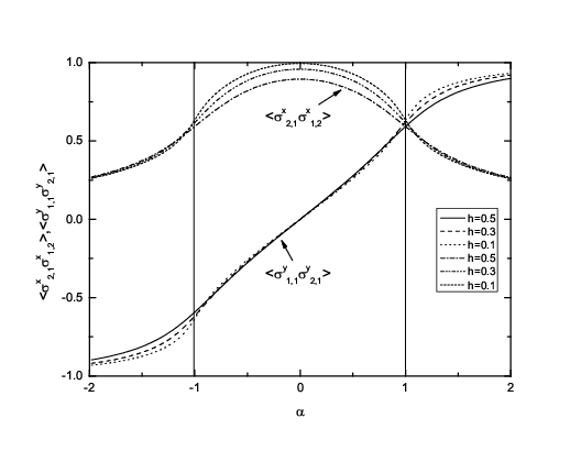
To explore the essential properties of QPT, we will calculate two GS pseudo-spin correlations $\langle\sigma_{2,1}^{x}\sigma_{1,2}^{x}\rangle$ and $\langle\sigma_{1,1}^{y}\sigma_{2,1}^{y}\rangle$. The numerical results for these two correlation functions versus $\alpha$ for different magnetic fields are presented in Fig. 8. We observe that $\langle\sigma_{1,1}^{y}\sigma_{2,1}^{y}\rangle$ is a odd function of $\alpha$, while $\langle\sigma_{2,1}^{x}\sigma_{1,2}^{x}\rangle$ an even one of $\alpha$. The crossing points of $\langle\sigma_{2,1}^{x}\sigma_{1,2}^{x}\rangle$ and $\langle\sigma_{1,1}^{y}\sigma_{2,1}^{y}\rangle$ curves deviate $\alpha=1$ in the presence of transverse field. The numerical results indicate that $\langle\sigma_{2,1}^{x}\sigma_{1,2}^{x}\rangle$ is sensitive to the external magnetic field in the range of $\alpha\in[-1,1]$, but insensitive in the other regions.

As done in Ref. [5], we also calculate the distance dependence of the pseudo-spin correlator $\langle\sigma_{2,1}^{x}\sigma_{1,2+r}^{x}\rangle$ with ABC for different size in terms of the Hamiltonian (1). As shown in Fig. 9 that the correlators at $\beta\rightarrow 1$ decay in an algebraic way in large $r$ regime, indicating a divergent correlation length when approaching the critical points. A power law behavior $\langle\sigma_{2,1}^{x}\sigma_{1,2+r}^{x}\rangle\propto r^{-\eta}$ is obtained with $\eta=1.00\pm 0.03$, indicating a second-order QPT.

Finally, we calculate the pseudospin magnetization $\langle\sigma^{z}\rangle=\langle\sigma_{1,n}^{z}\rangle+\langle\sigma_{2,n}^{z}\rangle$ and the magnetic susceptibility $\chi=\partial\langle\sigma^{z}\rangle/\partial h$. The magnetization $\langle\sigma^{z}\rangle$ as a function of the transverse field $h$ for $\alpha=1.0$ and $N^{\prime}=256$ is exhibited in Fig. 10. The magnetic susceptibility $|\chi(h)-\chi(h_{c})|$ versus $|h-h_{c}|$ shows a power law behavior. The exponent $\gamma$ is estimated to be $1.78\pm 0.05$ by the slop. It is interesting that it is very close to the magnetic susceptibility exponent $1.75$ in 2D classical Ising model. According to Eq. (17), we can also plot the similar scaling curve for 1D transverse field Ising model, which is given in the inset of Fig. 10 as well. A excellent agreement for the slop in the critical regime is clearly shown.

By using the method of mapping into a case with plural spin sites, we obtain the exact GS energy and the GS wave function of 1D compass model in a transverse magnetic field. The pseudo-spin liquid disordered ground state is the universal features in the 1D compass model. Meanwhile, we observe the second-order QPTs at ($\alpha=\pm 1,h=0$). The energy gap $\Delta$ will survive even in the thermodynamic limit for $h\neq 0$. It is useful for supporting naturally robust quantum information. The fidelity, the FS, the concurrence, and the block-block entanglement entropy are also calculated in terms of the obtained exact GS wave functions. The finite-size scaling analysis suggests the second-order QPT occurs by driving the transverse field. The pseudo-spin correlation functions, the distance dependence of the pseudo-spin correlators and the magnetization are also calculated. It is observed that the distance dependence of $\langle\sigma_{2,1}^{x}\sigma_{1,2+r}^{x}\rangle$ correlator displays a divergent correlation length when approaching the critical points. The obtained scaling exponents are nearly the same as those in the 1D transverse field Ising model, suggesting that these two models share the same universality class. The scaling exponent $c=1.0$ of the block-block entanglement entropy is the same as the critical XX chain with no magnetic field, which shows the different topological structure from the quantum Ising model. For the 2D compass model with a transverse field, the degeneracy of GS is removed because of the destruction of the symmetries. It is expected that the QPT becomes more weak and the first-order QPT is unlikely.

We acknowledge useful discussions with Prof. Lei-Han Tang. We also thank Prof. Perk for pointing out one problem in the original version of this paper. This work was supported by National Natural Science Foundation of China, PCSIRT (Grant No. IRT0754) in University in China, National Basic Research Program of China (Grant No. 2009CB929104), Zhejiang Provincial Natural Science Foundation under Grant No. Z7080203, and Program for Innovative Research Team in Zhejiang Normal University.

$*$ Corresponding author. Email:qhchen@zju.edu.cn

References

- [1] J. Dorier, F. Becca, and F. Mila, Phys. Rev. B 72, 024448 (2005).
- [2] H. D. Chen, C. Fang, J. P. Hu, and H. Yao, Phys. Rev. B 75, 144401 (2007).
- [3] B.Doucot, M. V. Feigel’man, L. B. Ioffe, and A. S. Ioselevich, Phys. Rev. B 71, 024505 (2005).
- [4] A. Mishra, M. Ma, F.-C. Zhang, S. Guertler, L.-H. Tang, S. L. Wan, Phys. Rev. Lett. 93, 207201 (2004).
- [5] W. Brzezicki, J. Dziarmaga, A. M.Ole, Phys. Rev. B 75, 134415 (2007).
- [6] R. Ors, A. C. Doherty, and G. Vidal, Phys. Rev. Lett. 102, 077203 (2009).
- [7] K. W. Sun, Y. Y. Zhang and Q. H. Chen, Phys. Rev. B 79, 104429 (2009).
- [8] E. Eriksson and H. Johannesson, Phys. Rev. B 79, 224424(2009).
- [9] W. L. You, and G. S. Tian, Phys. Rev. B 78, 184406 (2008).
- [10] G. Jackeli and G. Khaliullin, Phys. Rev. Lett. 102, 017205 (2009).
- [11] X. Y. Feng, G. M. Zhang, and T. Xiang, Phys. Rev. Lett. 98, 087204 (2007).
- [12] X. F. Shi, Y. Yu, J. Q. You, and F. Nori, Phys. Rev. B 79, 134431 (2009).
- [13] H. Bombin and M. A. Martin-Delgado, Phys. Rev. B 78, 115421 (2008).
- [14] J. Vidal, R. Thomale, K.P. Schmidt, and S. Dusuel, arXiv:0902.3547.
- [15] V. W. Scarola, K. B. Whaley and M. Troyer, Phys. Rev. B 79, 085113 (2009).
- [16] P. Buonsante and A. Vezzani, Phys. Rev. Lett. 98, 110601 (2007).
- [17] M. Cozzini, R. Ionicioiu, and P. Zanardi, Phys. Rev. B 76, 104420 (2007).
- [18] S. Chen, L. Wang, Y. J. Hao, and Y. P. Wang, Phys. Rev. A 77, 032111 (2008).
- [19] J. Preskill, J. Mod. Opt. 47, 127 (2000).
- [20] T. J. Osborne and M. A. Nielsen, Phys. Rev. A 66, 032110 (2002); A. Osterloh et al., Nature (London) 416, 608 (2002).
- [21] G. Vidal et al., Phys. Rev. Lett. 90, 227902 (2003); G. Vidal, ibid. 99, 220405 (2007).
- [22] V. E. Korepin, Phys. Rev. Lett. 92, 096402 (2004); G. C. Levine, ibid. 93, 266402 (2004); G. Refael and J. E. Moore, ibid. 93, 260602 (2004); P. Calabrese and J. Cardy, J. Stat. Mech. (2004) P06002.
- [23] A. Kitaev and J. Preskill, Phys. Rev. Lett. 96, 110404 (2006); M. Levin and X.-G. Wen, ibid. 96, 110405 (2006).
- [24] F. Verstraete, M. A. Martin-Delgado, and J. I. Cirac, Phys. Rev. Lett. 92, 087201 (2004); W. Dur et al., ibid. 94, 097203 (2005); H. Barnum et al., ibid. 92, 107902 (2004).
- [25] H. Q. Zhou, R. Ors, and G. Vidal, Phys. Rev. Lett. 100, 080602 (2008).
- [26] D. F. Abasto, A. Hamma, and P. Zanardi, Phys. Rev. A 77, 022327 (2008).
- [27] S. J. Gu, H. M. Kwok, W. Q. Ning, and H. Q. Lin, Phys. Rev. B 77, 245109 (2008).
- [28] T. Liu, Y. Y. Zhang, Q. H. Chen, and K. L. Wang, Phys. Rev. A 80, 023810(2009)
- [29] M. Nielsen and I. Chuang, Quantum Computing and Quantum Communication (Cambridge Univ. Press, Cambridge, 2000).
- [30] L. F. Zhang and P. Q. Tong, J. Phys. A 38, 7377 (2005).
- [31] A. Osterloh, L. Amico, G. Falci, and R. Fazio, Nature (London) 416, 608(2002); S. J. Gu, H. Q. Lin, and Y. Q. Li, Phys. Rev. A 68, 042330(2003).
- [32] N. Lambert, C. Emary, and T. Brandes, Phys. Rev. Lett. 92, 073602(2004).
- [33] G. Liberti, F. Plastina, and F. Piperno, Phys. Rev. A 74, 022324 (2006). J. Vidal and S. Dusuel, Europhys. Lett. 74, 817(2006)).
- [34] Q. H. Chen, Y. Y. Zhang, T. Liu, and K. L. Wang, Phys. Rev. A 78, 051801(R) (2008).
- [35] S. Sasaki, Phys. Rev. E 53, 168 (1996).
- [36] J. H. H. Perk, H. W. Capel, M. J. Zuilhof and Th. J. Siskens, Physica A 81, 319-348(1975).
- [37] S. Sachdev, Quantum Phase Transitions (Cambridge University Press, Cambridge, England, 1999).
- [38] P. Lou and J. Y. Lee, Phys. Rev. B 74, 134402 (2006).
- [39] G. Refael and J. E. Moore, Phys. Rev. B. 76, 024419 (2007).
- [40] E. Fradkin and J. E. Moore, Phys. Rev. Lett. 97, 050404 (2006).