Reduced density matrices and entanglement entropy in free lattice models
Abstract
We review the properties of reduced density matrices for free fermionic or bosonic many-particle systems in their ground state. Their basic feature is that they have a thermal form and thus lead to a quasi-thermodynamic problem with a certain free-particle Hamiltonian. We discuss the derivation of this result, the character of the Hamiltonian and its eigenstates, the single-particle spectra and the full spectra, the resulting entanglement and in particular the entanglement entropy. This is done for various one- and two-dimensional situations, including also the evolution after global or local quenches.
1 Introduction
Reduced density matrices contain the information on some part of a quantum system and are a basic tool in many-body physics. The ones commonly employed describe the properties of one or two selected particles in a many-particle system and allow to calculate important physical quantities like the total energy or the density correlations. These reduced density matrices (RDM’s) were first introduced by Dirac [1] and studied already in the 1930’s, see e.g. [2, 3]. In the usual terminology, they are just the static one- and two-particle correlation functions.
The RDM’s we want to discuss here are of a different type and refer to a different question. They arise if one divides a system in space, or, more generally, in Hilbert space, and asks how the two parts are coupled in the given wave function. This corresponds to the analysis by Schrödinger in 1935 [4] when he introduced the concept of entanglement. The general form of this coupling is given by the Schmidt decomposition which displays all entanglement features in a simple and transparent way. To obtain it in a specific case, one needs the RDM’s for the two regions in question.
The present interest in this problem, although it had also been a theme in quantum optics, arose in the beginning of the nineties in two seemingly disconnected areas, in the theory of black holes [5, 6, 7] and in the numerical investigation of quantum chains [8, 9]. In both cases, the motivation came from the wish to consider some subsystem which is in contact with its environment. For the quantum chains, this lead to the density-matrix renormalization group (DMRG) which can treat large systems with spectacular accuracy and revolutionized the field [10, 11]. A third input then came from the area of quantum information, where the structure of quantum states also plays a central role. This resulted in particular in a renewed and extensive study of the entanglement entropy [12, 13, 14] which is a simple and convenient measure of the entanglement and follows directly from the RDM eigenvalues.
The purpose of this article is to give a coherent account of the reduced density matrices just described for a class of models where they can be obtained in closed form. These are free fermions including the related spin chains and free bosons in the form of coupled oscillators. They will be considered either in their ground state or in certain other pure quantum states. In this case, the RDM’s are found to have a Boltzmann-like form with a certain free-particle operator in the exponent. The problem is thereby reduced to the study of this associated Hamiltonian and its characteristic features. The main property of interest is the eigenvalue spectrum since it determines the spectrum of the RDM itself and thus the entanglement properties, in particular the entanglement entropy. Both the spectra and the entropies will be presented for a variety of different situations. The problem on a lattice is very clear-cut. The partitioning is done by selecting two sets of discrete sites and there are no divergencies for finite sizes. On the other hand, there is only a small number of analytical results and one has to invoke numerics frequently. Lattice systems are also required for the DMRG, and the initial motivation for the studies was to understand the performance of this intriguing numerical method by looking at solvable models.
In section 2 we will provide some background on entanglement, the Schmidt decomposition and the RDM’s. Then, in section 3, we give the general form of the reduced density matrices for free fermions or bosons and discuss the methods for obtaining them. For quantum chains, this also contains relations to two-dimensional classical models. In section 4 we show the eigenvalue spectra for various one- and two-dimensional systems and discuss their typical appearance, their scaling behaviour and the change with the dimension. The characteristics of the single-particle eigenfunctions, the nature of the effective Hamiltonian and some further aspects are the topics of section 5. In section 6 we turn to the entanglement entropy and summarize the important results with emphasis on their relation to the spectra. Finally, in section 7, we review the temporal behaviour of the entanglement after different types of quenches. The material is drawn preferentially from our own studies and some of it also appeared in a recent book [15]. However, the scope is different here and a considerable number of figures were prepared exclusively for this review.
2 Background
In this section, we summarize the basic features of entangled states and reduced density matrices in order to create the frame for the results to be presented later. For more details, see e.g. the short review [16].
2.1 Schmidt decomposition
Consider a quantum system which is divided into two distinct parts 1 and 2. Then a state of the total system can be written
| (1) |
where and are orthonormal basis functions in the two Hilbert spaces. But a rectangular matrix can always be written in the form where is unitary, is diagonal and the rows of are orthonormal. This is called the singular-value decomposition and similar to the principal-axis transformation of a symmetric square matrix [17]. Using this in (1) and forming new bases by combining the with and the with , one obtains the Schmidt decomposition [18]
| (2) |
which gives the total wave function as a single sum of products of orthonormal functions. Here the number of terms is limited by the smaller of the two Hilbert spaces and the weight factors are the elements of the diagonal matrix . If is normalized, their absolute magnitudes squared sum to one. The entanglement properties are encoded in the set of . Only if all except one are zero, the sum reduces to a single term and is a product state, i.e. non-entangled. In all other cases a certain entanglement is present and if all are equal in size, one would call the state maximally entangled. Of course, this refers to a particular bipartition and one should investigate different partitions to obtain a complete picture.
2.2 Reduced density matrices
The entanglement structure just discussed can also be found from the density matrices associated with the state . This is, in fact, the standard way to obtain it. Starting from the total density matrix
| (3) |
one can, for a chosen division, take the trace over the degrees of freedom in one part of the system. This gives the reduced density matrix for the other part, i.e.
| (4) |
These hermitian operators can be used to calculate arbitrary expectation values in the subsystems. Moreover, it follows from (2) that their diagonal forms are
| (5) |
This means that
- •
and have the same non-zero eigenvalues
- •
these eigenvalues are given by
Therefore the eigenvalue spectrum of the gives directly the weights in the Schmidt decomposition and a glance at this spectrum shows the basic entanglement features of the state, for the chosen bipartition. For this reason, it has also been termed “entanglement spectrum” recently [19]. One also sees that the appearing in (2) are the eigenfunctions of the . For the single-particle RDM’s mentioned in the introduction, these eigenfunctions are known as “natural orbitals” in quantum chemistry [20].
In the DMRG algorithm, these properties are used to truncate the Hilbert space by calculating the , selecting the states with largest weights and deleting the rest. This procedure is expected to work well if the total weight of the discarded states is sufficiently small. Therefore the form of the density-matrix spectra is decisive for the success of the method.
It is interesting that Schmidt himself already worked with the RDM’s. Studying coupled linear integral equations, he derived a spectral representation of the form (2) for an unsymmetric kernel in terms of the eigenfunctions of the two symmetric operators and . His paper (which is based on his doctoral thesis with Hilbert) also contains the recipe for the best approximation as it is used in the DMRG.
2.3 Entanglement entropy
Whereas the full RDM spectra give the clearest impression of the entanglement in a bipartite system, it is also desirable to have a simple measure which condenses this information into one number. This can be achieved by generalizing the usual (von Neumann) entropy definition to reduced density matrices. The entanglement entropy therefore reads:
| (6) |
where the trace has been rewritten as a sum using the eigenvalues . The most important properties are as follows.
- •
The entropy is determined purely by the spectrum of , which is known to be identical to the spectrum of . Therefore holds for arbitrary bipartitions and one can simply write and talk of the entanglement entropy.
- •
The entropy vanishes for product states, and has a maximal value of if one has non-zero eigenvalues which are all equal, for . Using this, one can write in general , thereby defining an effective number of states coupled in parts and . This gives a simple interpretation to .
Although there are other entanglement measures [21], the entropy is the standard one for bipartitions and will be discussed in detail later. It is important to keep in mind that it measures a mutual connection and will, in general, not be proportional to the size of a subsystem.
3 RDM’s for free lattice models
3.1 Systems
In the following we consider models with a Hamiltonian which is quadratic in either fermion or boson operators and thus can be diagonalized by a Bogoliubov transformation. In principle, these can be quite general, but we will concentrate on the following physically important systems
- •
Fermionic hopping models with conserved particle number and Hamiltonian
(7) where the symbol denotes nearest neighbours. Apart from homogeneous systems we will consider dimerized chains, where alternates between , and the case of single defects.
- •
Coupled oscillators with eigenfrequency and Hamiltonian
(8) These are systems with an optical spectrum and bosonic pair creation and annihilation.
- •
Spin one-half chains which are equivalent to free fermions via the Jordan-Wigner transformation. The most general one is the XY chain with a Z field, described by
(9) where the are Pauli matrices at site . For this reduces to the XX model, corresponds to (7) with nearest-neighbour hopping and can also model hard-core bosons. For , it contains pair creation and annihilation terms. For it becomes the Ising model in a transverse field (TI model) which we write, in a slightly different notation
(10)
The solubility of the models in itself does not yet mean that the RDM’s are easily accessible. For example, they have been considered in the critical XXZ spin chain, but the formulae are very complicated, see [22, 23]. The free lattice models, however, have eigenstates with special properties which permit to make a simple general statement.
3.2 General result
For these free-particle models, the reduced density matrices for the ground state can be written
| (11) |
Here is the number of sites in subsystem and the operators , are fermionic or bosonic creation and annihilation operators for single-particle states with eigenvalues . The ’s are related to the original operators in the subsystem by a canonical transformation. Thus has the form of a thermal density matrix with an effective Hamiltonian which is of the same free-particle type as . In (11) it is already given in diagonal form. The constant , written in analogy to thermodynamics, ensures the correct normalization .
This form of is rather suggestive since one has a similar situation as for a system in contact with a thermal bath. However, no assumption about the relative sizes of the two coupled systems enters here. More importantly, the operator is not the Hamiltonian restricted to the subsystem . Therefore (11) is not a true Boltzmann formula. Nevertheless, the problem has been reduced to the study of a certain Hamiltonian and its thermodynamic properties. The features of will be the topic of the next chapters. Generally, one can say that it corresponds to an inhomogeneous system even if the subsystem it describes is homogeneous. This will be seen in more detail in section 5.2. Here we first discuss how one arrives at (11). These considerations will also show that validity of (11) goes even beyond the ground state.
3.3 Methods
Basically, there are three methods to obtain the reduced density matrices.
(I) Integration over part of the variables according to the definition (4). This can be done e.g. for coupled harmonic oscillators [24, 25]. In this case the ground state is a Gaussian in the normal coordinates, provided no normal frequency vanishes. In terms of the original coordinates of the oscillators, it has the form
| (12) |
Here is a normalization constant and the matrix is the square root of the dynamical matrix associated with the potential energy. By forming and integrating out e.g. the variables one obtains which is again a Gaussian. With proper linear combinations of the coordinates, it contains only squares and differences . Early treatments worked with this integral operator [5, 6]. However, one can convert the differences into second derivatives and thereby obtain the differential operator
| (13) |
where the exponents become quadratic expressions in terms of boson operators. A diagonalization then gives the single exponential (11) with describing a collection of new harmonic oscillators. Their eigenfrequencies follow from by dividing it into the submatrices , and , according to whether the sites are in part 1 or in part 2. Then the matrix has the eigenvalues .
If , there is just one such oscillator with a frequency which differs from . Its eigenstates have a different spatial extent and may therefore be called “squeezed”. For the resulting Schmidt decomposition of in terms of these states can easily be written down and is well known, see e.g. [26, 27].
The method can also be used for systems of non-interacting fermions. In this case one first has to write the ground state in exponential form and then use Grassmann variables for the integration [28, 29].
(II) Via correlation functions [30, 12, 31]. The simplest case is a system of free electrons hopping on lattice sites in a state described by a Slater determinant. In such a state, all many-particle correlation functions factorize into products of one-particle functions. For example,
| (14) |
If all sites are in the same subsystem, a calculation using the reduced density matrix must give the same result. This is guaranteed by Wick’s theorem if is the exponential of a free-fermion operator
| (15) |
where and are sites in the subsystem. With the form of fixed, the hopping matrix is then determined such that it gives the correct one-particle correlation functions . The two matrices are diagonalized by the same transformation and one finds (see also [29])
| (16) |
The same formula also relates the eigenvalues and of and . Expressed differently, the follow from the equation
| (17) |
If there is pair creation and annihilation, one has to include the ’anomalous’ correlation functions and . To reproduce them, the operator then must also contain pair terms. Diagonalizing it in the usual way [32], one finds that the single-particle eigenvalues follow from two coupled equations, which can be combined into a single one. For real this reads
| (18) |
and reduces to the previous result (17) if vanishes. Alternatively, one can work with Majorana operators [12, 13] and and form the correlation matrix . Restricted to the subsystem, it contains the same elements as the two matrices in (18) but arranged differently. Writing , the matrix of the subsystem has the eigenvalues .
This method is very general. It works in any dimension, for arbitrary quadratic Hamiltonians, for all states which are Slater determinants, and even at finite temperature. Thus it has been used in a large number of situations ranging from homogeneous chains to defect problems, random systems, higher dimensions and the time evolution after a quench.
Factorization properties as in (14) are well-known for Gaussians, and therefore the approach is equally applicable to coupled oscillators in the ground state (12). Thus must be the exponential of a bosonic operator (as found in (I)) and is again determined such that it reproduces the correlation functions, in this case those of positions and momenta, and . In analogy to (18) the single-particle eigenvalues then follow from [33, 30, 34]
| (19) |
Since for the total system and , the matrix on the left side of (19) is seen to be the restriction of to the subsystem multiplied by the restriction of its inverse. This is exactly the expression given in (I). As in the fermionic case, one can also combine coordinates and momenta, which are analogous to the Majorana variables, and consider the corresponding correlation matrix, usually called covariance matrix. Its reduction to diagonal form is a well-known problem in mathematics [35] and the resulting are also referred to as symplectic eigenvalues [36, 37].
(III) Via classical statistical models [40, 41]. In one dimension one can exploit the relations between quantum chains and two-dimensional classical models. The starting point is a discrete version of a path-integral representation.
Consider a quantum chain of finite length and imagine that one can obtain its state from an initial state by applying a proper operator many times. If is the row-to-row transfer matrix of a classical model, one has thereby related to the partition function of a two-dimensional semi-infinite strip of that system. The total density matrix is then given by two such strips. This is sketched on the far left of Fig.1. The reduced density matrix, e.g. for the left part of the chain, follows by identifying the variables along the right part of the horizontal edges and summing them, which means tying the two half-strips together. In this way, is expressed as the partition function of a full strip with a perpendicular cut, as shown half left in the figure.
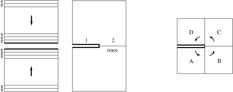
This procedure works for the ground state of a number of integrable quantum chains. For example, the TI chain can in this way be related to a two-dimensional Ising model on a square lattice which is rotated by with respect to the horizontal [41]. In the same way, a chain of coupled oscillators is connected with a two-dimensional Gaussian model [24] and an XY chain with an Ising model on a triangular lattice [42]. Analogous correspondences link XXZ, XYZ and higher-spin chains to vertex models [41, 43, 44]. To use these relations, however, one needs a way to actually calculate the resulting partition function. This is possible with the help of the corner transfer matrices (CTM’s) introduced by Baxter [45]. These are partition functions of whole quadrants as shown on the right of Fig.1, or of sextants, if one is dealing with a triangular lattice. By multiplying these transfer matrices one can then obtain the reduced density matrix for a half-chain as
| (20) |
Since is given by an infinite strip, one also needs infinite-size CTM’s in this relation. But exactly in this limit they are known for several non-critical integrable models and have the form
| (21) |
where contains the anisotropy of the two-dimensional system. This is a consequence of the star-triangle relations on which the integrability rests [46]. This approach gives in the original variables, see section 5.2, and explicit expressions for the single-particle eigenvalues in the diagonalized form. According to the derivation, it applies to one-half of an infinite chain, but in practice the chain has only to be much longer than the correlation length.
Summing up, we have shown how to arrive at (11) and how to obtain the . The eigenstates of and their eigenvalues then follow by specifying the occupation numbers of all single-particle levels. The analytical result for just mentioned is exceptional. For finite subsystems beyond one or two sites, one has to find the numerically. This leads to a characteristic difficulty, because the eigenvalue equations in (II) contain hyperbolic functions which approach for large . As the subsystem size grows, more and more values lie (exponentially) close to , and can only be obtained reliably with special techniques [47]. Therefore the values of the in most of the following figures do not exceed 20-30.
4 Spectra
In this section we give an overview of the single-particle spectra and the full -spectra for various situations. These include different dimensions, critical and non-critical systems and the geometrical shape of the subsystem. We will focus on the because these are the primary quantities.
4.1 One dimension
(I) Non-critical chains.
For infinite TI, XY and oscillator half-chains, the CTM approach gives the universal formula
| (22) |
where . Thus one has equidistant levels and in a plot the dispersion is strictly linear.
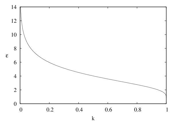
The only free parameter is the level spacing which depends on the details of the model. It is given by
| (23) |
where denotes the complete elliptic integral of the first kind, and . The elliptic modulus with is given in the TI model by
| (24) |
In the XY model, the ordered region is subdivided by the so-called disorder line and one has to distinguish three cases
| (25) |
Here the last formula comes from a different approach [48, 49]. For the oscillator chain, is the nearest-neighbour coupling and one has to put . In this case, there is no ordered region. In all models, the critical point is given by and since diverges for , the level spacing vanishes there and the dispersion curve becomes flat. The complete behaviour of is shown in Fig. 2.
Results for finite TI chains are shown in Fig. 3 on the left. The linear behaviour is perfect for the smallest . As one comes closer to the critical point, the slope decreases as predicted, but there are also deviations from the linearity for large . Thus the linear region shrinks and is no longer visible at the critical point. This is the typical finite-size scenario in these models. On the right side, the resulting , ordered by magnitude, are shown. One can see a rapid decrease with which is fastest for the smallest but is still impressive at criticality (note the vertical scale). This means that a Schmidt decomposition could be truncated safely after about 10 terms and is the basis for the fantastic performance of the DMRG in this case [50].


The lowest -curve also shows a step structure with plateaus which become longer with . These are a consequence of the equidistant levels, a certain eigenvalue of can then be realized by different combinations of . The degeneracy is given by the number of partitions of an integer into other (odd or even) integers. Using asymptotic formulae for the , one finds the leading large- behaviour [51]
| (26) |
where . The same result with a different constant holds for bosons. If the dispersion is not strictly linear, the steps are smeared and a rather smooth spectrum is obtained.
An important new feature appears in the -spectra, if the subsystem is a segment in a chain. Then a two-fold degeneracy is found, at least for the lowest eigenvalues. The reason lies in the form of the eigenfunctions, which are concentrated near the ends, as will be demonstrated in section 5. This leads to a degeneracy of the , with a factor of 2 for each which is involved, and therefore to a significantly slower decay.
For the spin chains, there are cases where the ground state simplifies and becomes a doublet of product states. Then one is zero, while all others diverge. As a consequence, all except two collapse to zero. This happens not only in the TI model for , but also in the XY model on the disorder line [28]. If the result were not known, one could locate the line from the behaviour of the spectra.
Finally, we note that also a dimerized half-filled hopping model shows such equidistant because one can relate it to the TI model via the correlation functions. The parameter is then given by , where is the dimerization parameter.
(II) Critical chains.
In critical systems, the size of the subsystem affects not only the upper part of the single-particle spectrum. This is shown in Fig. 4 for a segment in a half-filled hopping model, or XX chain.


The eigenvalues follow in this case from the simple correlation matrix
| (27) |
where for half filling. One sees that the whole dispersion curve is shifted towards the horizontal axis and becomes flatter as the length increases. The shift is not rapid, the first few eigenvalues vary as with somewhat different constants around 2.5. From a continuum approximation for the eigenvalue problem, one obtains the asymptotic formula
| (28) |
which can also be derived with conformal considerations [52]. A similar expression for bosons was given in [53]. The formula is also valid for a segment of sites at the end of a chain, if one substitutes , which increases the values roughly by 2. It predicts the behaviour, but also a linear dispersion as in the non-critical case. In practice, this can only be seen if in addition to also is large, which requires huge sizes. Nevertheless, it is an important guide for the understanding of the situation and will be used again later. Formulae of this type and the numerical difficulties in verifying them are known from studies of critical finite-size CTM’s [54, 55, 56].
Although the change of the is slow, it has a clear effect on the spectra, as seen on the right of the figure. The decay becomes significantly slower for larger systems, which means that the entanglement grows with the size. Invoking conformal results, one can obtain the functional form of the -spectrum [57, 58]. Asymptotically, (26) is still valid, but now varies with the length. Therefore the DMRG method does not work as well in this case, although it still can handle sizes of .
Finally we want to show how certain modifications of the ground state affect the spectra. In the previous cases, the system was always half filled, which leads to a symmetric spectrum ( appear) [29]. If the filling is varied in (27), one finds that the -dispersion curve is moved up or down in a similar way as the Fermi level, see Fig. 5. For a completely full or empty system, which is a product state (in spin language all spins are up or down), the are all infinite and becomes a Kronecker symbol, , as it should.


If the Fermi sea consists of several disconnected parts, one finds degeneracies in the eigenvalues, if empty and full regions in momentum space have equal size. This is shown in Fig. 5 on the right. It looks as if one had several independent kinds of particles. Effectively, the dispersion then rises only with a fraction of the slope. The same holds in the case of non-equal Fermi seas, where the degeneracies are washed out. Such a situation occurs, for example, for the ground state of the chain with an energy current [59]. As in the previous examples, the then decrease more slowly and the entanglement becomes larger.
If one modifies the hopping between the segment and the environment at one interface, one can interpolate continuously between a homogeneous chain and one with an open end. [60]. The -spectrum in this case is shown in Fig. 6 on the left. As the bond is weakened, a region with a steeper initial ascent appears before the curve follows the pattern without defect. This region can be associated with the developing free end and remains when the bond is cut completely. If, on the other hand, the bonds at both interfaces are weakened, the dispersion is shifted upwards resp. downwards as a whole and a gap develops. In the decoupling limit it goes to infinity and the entanglement vanishes.


4.2 Two dimensions
(I) Non-critical systems
The simplest two-dimensional system consists of a set of uncoupled identical parallel chains, all divided at the same point such that the subsystem has the form of a half-strip [61]. This is the usual DMRG geometry. The combined RDM is then a product of the individual ones and becomes a sum
| (29) |
where is the chain index. Since , the single-particle eigenvalues are simply -fold degenerate. For free particles, a coupling of the chains does not change this situation because one can separate the system into new independent chains by a Fourier transformation in the perpendicular direction [25, 62]. The index in (29) then becomes the Fourier index . Only will depend on and the -fold degenerate levels will become bands.
For coupled oscillators and an infinite half-strip, the problem can in this way be solved exactly by invoking the one-dimensional results. One only has to determine the elliptic parameter for each Fourier component from the coupling in the chain direction and the frequency via
| (30) |
Numerical results for a system of 10 chains with actually finite length are shown in Fig. 7.

The coupling of the chains was varied and one can see nicely, how the plateaus with 10 levels develop into bands and a rather smooth, roughly linear curve results in the isotropic case. The initial plateaus, combined with the large freedom in the bosonic occupation numbers, lead to even larger plateaus in the -spectrum. In the isotropic case, one can derive an asymptotic formula as (26) by assuming a strictly linear behaviour with a slope
| (31) |
Then one finds (26) with a coefficient . The crucial difference is that depends inversely on the width, which makes the decay of the exceedingly slow for wide systems. The entanglement becomes correspondingly high. This is a general feature and will be taken up again in section 6. For the DMRG it means that the width of the strip puts a fundamental limit on its applicability.
For subsystems in the form of squares embedded in an infinite lattice, one can obtain similar results by solving the equation (19) numerically. One finds again bands as in Fig. 7, but the number of states in the lowest bands is now given by , which one recognizes as the the number of boundary sites. Plotting the as a function of the scaled index , the results fall essentially on top of each other. This is the same behaviour as for the single straight boundary, where enters. It is a clear indication that the single-particle states are associated with the interface between the subsystem and its surrounding, as in one dimension.
(II) Critical systems
In this case one finds similar features which we will exhibit for the hopping model on a square lattice. The isotropic half-filled model has the well-known quadratic Fermi surface with corners at and in momentum space. This gives the correlation function as the product of two one-dimensional ones as in (27)
| (32) |
where and are integers. If the model is anisotropic, the Fermi surface is more complicated and one momentum integration has to be done numerically. With these functions one can calculate the spectra for arbitrary subsystems embedded in an infinite lattice. For half filling, the spectra are again symmetric, i.e. the eigenvalues occur in pairs .
Fig. 8 shows results for squares, plotted to exhibit the scaling behaviour. On the left, the are shown as a function of the scaled index . One can see low-lying bands which all have the same horizontal length 1 and thus contain states. However, their height still varies with . Only by plotting they all collapse on one curve, as shown on the right. This demonstrates that, on the one hand, the linear size enters as in the non-critical case, but that also the inverse logarithmic dependence on found in one dimension remains. As a result, logarithmic corrections appear in the entanglement entropy, see section 6. Note also that enters, and not as before. This is most obvious in a band of eigenvalues which are exactly zero (the figure shows only one-half of it). The latter feature is peculiar to the square and does not occur for rectangles, where the dispersion rises smoothly from zero.


The resulting spectrum of is shown in Fig. 9 for three relatively small systems. For the square, all eigenvalues are displayed and the s-shaped curve actually reflects the symmetry of the spectrum. The system gives much smoother results which can be fitted well by the law (26). For it, and also for the system, the curves drop only to a value of about for around , which is to be compared with the one-dimensional results of Fig. 4, where this value is reached already at for . The same feature is found for other geometries [28, 47]. This shows very clearly the basic difference between one and two (and also higher) dimensions.

5 Further aspects
5.1 Single-particle wave functions
(I) Chains
The eigenfunctions associated with the have a particular nature. In Fig.10 they are shown for the smallest in the case of a segment in a half-filled hopping model. On the left, the model is dimerized, i.e. non-critical, and one sees that the amplitude is concentrated near the two interfaces to the remainder and almost zero in the middle. This feature persists even in the homogeneous critical case seen on the right, although there is now a slow decay into the interior. For the highest , on the other hand, the amplitude is concentrated in the centre of the subsystem and the eigenfunction resembles a Gaussian. The same pattern can be seen in oscillator chains [25, 63, 36]. It is very suggestive, since it means that the states which are most important in the entanglement are those closest to the boundary. The whole entanglement appears as a phenomenon taking place within a layer whose width is given by the correlation length.


A lattice result for in the hopping model is only available in the case which occurs for odd [52]. The wave function then is u-shaped and vanishes at every second site, see [64]. However, one can derive an expression in the continuum limit. Putting , it reads for a segment located between and [52]
| (33) |
Such logarithmic oscillations were found earlier in CTM studies related to the TI [56] and the oscillator half-chain [65]. In the latter case, which was also treated in [53], the square-root prefactor is absent.
(II) Planar systems
It is clear that the basic feature, namely the concentration near the interface, will also be found in two dimensions. As an example, Fig. 11 shows the

situation for the states which occur for a quadratic subsystem in a planar hopping model. Due to the degeneracy, the individual states are not uniquely defined and one has to consider all simultaneously. The maxima at the boundary are clearly visible and one has the same u-shaped pattern as in the one-dimensional case. In addition, there is a slight enhancement along the diagonals. In general, the eigenfunctions have variations parallel to the interface which are related to the square symmetry. To bring out their “radial”behaviour one has to calculate the analogue of a radial distribution function. One then sees, apart from a small bump in the centre, a clear increase towards the boundary for all low-lying bands. This will be even more pronounced in a non-critical system.
5.2 Nature of
The eigenfunctions presented in the previous subsection have their origin in a particular form of the effective Hamiltonian, which we now address. In the CTM approach it is possible to give an explicit expression for . This is done by considering (21) in the limit of a very anisotropic system [66, 67, 68]. For the TI half-chain this leads to the result
| (34) |
where the constant depends on . Therefore also describes a TI chain, but an inhomogeneous one, with coefficients which increase linearly away from the interface. In the two-dimensional problem, this reflects the wedge-shaped geometry. In the RDM context, it suppresses the influence of sites far in the interior because enters exponentially into . This Hamiltonian can also be diagonalized directly [67, 68] and one recovers the result (22) for . In the limits and , the level structure (22) can directly be read off the coefficients in (34).
For any finite subsystem, can in principle be determined numerically. This is particularly simple for the homogeneous hopping model. Then the matrix elements follow from the correlation-matrix eigenfunctions via
| (35) |
The result for a segment in a chain is shown on the left of Fig. 12.


The dominant elements are those for nearest-neighbour hopping and vary roughly parabolically. This is the generalization of the linear law in the semi-infinite chain to this geometry. However, there is also hopping to more distant neighbours, although with rapidly decreasing amplitude. If the segment is located at the end of a chain, one finds the same behaviour but with only one-half of the parabola, i.e. the hopping saturates at the free end. The situation for a square in a two-dimensional lattice is shown on the right of the figure. Going parallel to an edge, the hopping in this direction varies again parabolically. It is smallest close to the edge and largest halfway in between the edges. This shows that the inhomogeneity in always follows the same pattern. One finds it also in the XXZ model with [69].
In the XX chain, one can actually show that for a segment commutes with the operator,
| (36) |
where the hopping is strictly only to the nearest neighbours and has exactly parabolic form [52]. Thus they have common eigenfunctions, and the result (33) was actually found from . Also the low-lying eigenvalues are related, and it could be that in the limit both operators become identical up to a factor. One cannot check that numerically, however, because then large appear which are not accessible, see section 3.
5.3 Definition of a temperature
It has been pointed out in section 3 that is not a true Boltzmann operator, since differs from the Hamiltonian , as shown above. However, if the single-particle excitations have the same functional form, one can bypass this argument. This is the case for the homogeneous hopping model [70]. Then the vary linearly for large according to (28) and the same holds for the single-particle energies in in the vicinity of the Fermi point. For hopping to nearest neighbours with matrix element these are, in the subsystem, given by
| (37) |
Therefore, one can write with an effective temperature
| (38) |
which depends on the length of the subsystem and vanishes for . Therefore can be regarded as a true grand canonical Boltzmann distribution for all expectation values, where only the small single-particle energies are important and the wave functions do not play a role. This holds, for example, for the particle-number fluctuations in the subsystem, which vary as at finite temperatures. Inserting (38), this is turned into the -behaviour for the segment in the chain.
5.4 Thermal states
Although our interest is in ground-state properties, it is instructive to see what happens if one calculates for a system at a finite temperature. This is quite easy with the correlation function approach, and the resulting spectra for the homogeneous half-filled hopping model with are shown in Fig. 13.

The steepest curve is the ground-state result. As the temperature is increased it flattens, bends over and assumes the shape of the dispersion for the single-particle energies in . In fact, one can write, expanding the Fermi function for
| (39) |
which has eigenvalues in the subsystem
| (40) |
and gives
| (41) |
In other words, for high temperature
| (42) |
which is a very plausible result. Apart from the shape of the spectrum, the essential point is that the level spacing is reduced from a value of order one to . Such a situation is also found in quenches, see section 7.
6 Entanglement entropy
In this section, we show how the properties of the RDM spectra seen in section 4 translate into in the behaviour of the entanglement entropy. Due to the form of the it is given by the same expression as in statistical physics
| (43) |
where the upper(lower) sign refers to fermions(bosons). From this formula, one can immediately draw two general conclusions
- •
The largest contributions come from small (corresponding to high temperature in usual thermodynamics). Therefore the entropy will be particularly large in critical systems. For fermions its maximum value of is reached if all vanish.
- •
If all are -fold degenerate, the value of is times its value without degeneracy. This answers e.g. how compares for one or two (noncritical) interfaces, or for one or two Fermi seas.
(I) One dimension
Analytical results can be given for the non-critical half-chains with the spectrum (22). The sums then lead to elliptic integrals [60] and one obtains for fermions in the disordered region
| (44) |
while for bosons the formula is
| (45) |
A similar expression with an additional contribution of coming from the eigenvalue holds in the ordered region. Also the results for XXZ and XYZ chains [72, 43] can be brought in this form. The entropy for the anisotropic XY chain with can be written as the sum of the expressions in the ordered and the disordered region [42, 71]. A plot of , based on a numerical evaluation of the sums, was first shown in [72]. Curves for the XY model can be found in [73]. The case of a segment in an XY chain was treated even before the half-chain. Using the correlation matrix and solving a Riemann-Hilbert problem, was obtained as an integral over theta functions [48, 49]. This is equivalent to the half-chain result multiplied by two.
In the disordered region there is little difference between fermions and bosons. The values of are typically of order one or smaller, so that the corresponding ground states have states in the Schmidt decomposition. This reflects the rapid decay of the spectrum in Fig. 3. An exception is only the vicinity of the critical point. As anticipated, becomes large there and actually diverges for this geometry. The formulae give for
| (46) |
where for the TI model and for the bosons. Since the correlation length varies as , the logarithm is of the form [72].
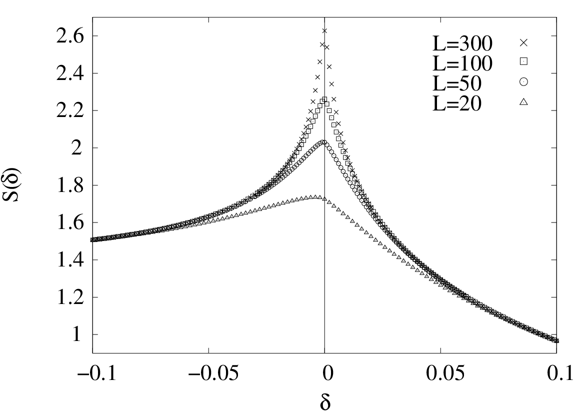
The behaviour for a finite subsystem is shown in Fig. 14 for segments in a dimerized hopping model. In this case, no longer diverges at criticality but shows a maximum which becomes higher with increasing . The size dependence at the critical point can be obtained in a very simple way [53]. Using the asymptotic form (28) of the in (43) and converting the sums into integrals gives
| (47) |
and since both integrals equal one finds
| (48) |
On the lattice, this behaviour was first found numerically [12, 13] and then by using the asymptotic properties of the correlation matrices [74, 75]. The general formula for critical chains is
| (49) |
Here is the central charge, the number of contact points between the (singly-connected) subsystem and the remainder of the chain, and a non-universal constant which depends on the model parameters and the geometry. An estimate for can be obtained if one replaces in (47), using the scaling found for the first few eigenvalues. This gives for the hopping model, whereas the correct value is . As the numerics show, the logarithmic behaviour of can already be observed in relatively small systems, where (28) is not yet valid. Since it holds for all conformally invariant models [7, 72] the formula (49) is a central result.
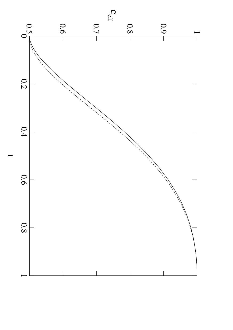
The interpolation between one and two contact points via a modified bond has already been discussed in section 4.1. Regarding the entropy, it can be described by an effective central charge in (49) which varies continuously between 1/2 and 1. The spectrum on the left of Fig. 6 then leads to the result in Fig. 15.
A formula for based on boundary conformal theory was given in [76]. The problem was also generalized to the case of two coupled planes [77]. Completely inhomogeneous systems were studied in the form of chains with extended defects [78], gradients [79], aperiodic [80] and random [81, 82, 83] couplings. On the other hand, one can consider situations where the subsystem is not singly connected and thus has many contact points. For comb-like geometries, the leading term in then becomes proportional to [84]. For example, if the sites of the subsystem are two lattice spacings apart, one has in the hopping model. This is a direct consequence of (27) which reduces to and gives for all . Conformal results for multiple intervals are reviewed in [58].
(II) Two dimensions
The influence of the interface on the spectra in two dimensions has already been demonstrated in section 4.2. In the entanglement entropy, it leads to the famous “area law” which has been the topic of many investigations, see [85] for a recent review. Consider, for example, the non-critical half-strip of oscillators. Each band of contributes an amount of order to which thereby becomes proportional to the length of the interface. Expressed differently, is the sum of the individual -chain entropies and can be written, for large ,
| (50) |
For a square-shaped subsystem where the lowest band contains as many states as there are interface sites, one obtains an analogous result.
The argument also holds for critical systems [62]. Regarding a two-dimensional hopping model as a system of coupled chains, the Hamiltonian reads, for ,
| (51) |
Thus for each -value one has a chain with a chemical potential . This affects the filling but does not change the -behaviour of , which therefore becomes proportional to . This is still an area law, but the occurrence of the second length disturbs the picture somewhat. The same holds for a square subsystem with the spectrum found in Fig. 8. There the number of states scales as but the value of the as . Thus one finds logarithmic corrections to the area law. This was proven exactly by constructing bounds on [86, 87, 88] and an expression for the prefactor was given in [87]. The problem was also investigated numerically in two [39, 89] and three [89] dimensions, and the presence of the logarithm traced to a finite Fermi surface in the system. For bosonic systems, on the other hand, no logarithmic corrections were found in the critical limit.
Finally, we want to comment briefly on the largest eigenvalue of the RDM, which has a close relation to . It plays a role in the so-called single-copy entanglement, where one asks which maximally entangled state one can reach from an initial state [90]. From (11) one sees that
| (52) |
where is the smallest eigenvalue of . This can be evaluated for the non-critical half-chains in the same way as . For example, putting , one finds in the bosonic case
| (53) |
In the critical limit, this diverges as and one finds that . The same holds for fermions [90, 91]. One can show that this is a general result for conformally invariant systems [91, 92, 93].
7 Entanglement evolution
In this last chapter we present results on the entanglement evolution after a change of the Hamiltonian . This can be treated via correlation functions as before and leads to interesting phenomena. The simplest case is a quench, where the change is instantaneous and generates a unitary time evolution . If is also a free-particle operator, the arguments work as before [94] and the RDM has the exponential form (11) as in equilibrium but with a time dependent operator
| (54) |
In the case of particle conservation, the eigenvalues follow again from the restricted correlation matrix, but now taken at time
| (55) |
Therefore, one only needs to determine the time evolution of the operators in the Heisenberg picture. In the following we discuss three different situations.
7.1 Global quench
In a global quench, the system is modified everywhere in the same way, a situation which can actually be realized in optical lattices [95]. Then the initial state becomes a highly excited state of with an extensive excess energy.
An example which illustrates the situation very well is a hopping model which is initially fully dimerized () and then made homogeneous (). The time evolution of the correlation matrix is then given explicitly in terms of Bessel functions [96]
| (56) |
The resulting single-particle spectra are shown on the left of Fig. 16. One sees that the dispersion is linear near zero and that its slope decreases with time. This leads to the initial increase of the entropy shown on the right of the figure. For times , however, the approach a limiting curve and saturates. The asymptotic form of the spectrum can be obtained from the tridiagonal correlation matrix as in section 5.4
| (57) |
leading to
| (58) |
The spacing of the is proportional to and gives an extensive entropy , a value which was also found in [94] for a similar quench in the TI model. An initial state where the sites are alternatingly full and empty, would even give the maximal possible value .


The build-up of an extensive entropy is a typical signature of global quenches. It was given a phenomenological description in terms of emitted pairs of quasiparticles which create entanglement between the subsystem and the remainder of the system [94, 58]. In our case these quasiparticles have maximum velocity . This simple picture also accounts for the “light-cone effect” [97, 98] reflected in the entropy at , where the linear increase turns into a saturation. If one starts from an inhomogeneous state the increase of can also be non-linear [79]. A closed expression for in the XY model was given in [99].
From the extensivity of one might conjecture a relation of the quench state to a true thermal state. But a comparison of the spectra in Figs. 13 and 16 shows that, apart from the linear region, they are different. A calculation of via (35) shows that it has long-range hopping which decreases as in the interior. However, there are cases, where the final effective Hamiltonian resembles . This happens e.g. if one starts from a chain with alternating site energies . Then one finds that for large the asymptotic have the form (41) with . This explains the observations in [100]. In general, the emergence of a after a global quench may still be viewed as a local thermalization and is a rather general feature of one-dimensional integrable systems, see e.g. [101, 102] for a rigorous treatment.
7.2 Local quench
A very different behaviour is obtained if one makes sudden local changes in the system, for example by removing defects in a hopping model. The resulting entanglement evolution has been investigated for various situations and geometries [96, 103, 104, 58]. We will consider here the case where a finite segment is joined to an infinite half-chain either on one or on both sides [104]. These two setups will be called the semi-infinite and the infinite geometry, respectively.
The time evolution of the Fermi operators is again given in terms of Bessel functions, and in the infinite geometry the correlation matrix reads
| (59) |
The double sum over all sites has in this case to be evaluated numerically. In the semi-infinite geometry, a similar expression is obtained.
On the left of Fig. 17 we show the low-lying single-particle spectrum for the semi-infinite case on a logarithmic time scale. Since the segment is initially unentangled, all first drop and evolve to a transient regime up to where all but one relax to the stationary eigenvalues of the equilibrium chain. The remaining anomalous eigenvalue evolves rather slowly showing avoided crossings with the already relaxed levels. The large-time behaviour is therefore characterized by a slow approach to the local equilibrium state.


The resulting entropy evolution in the transient region is shown on the right of Fig. 17. For both geometries one can see a plateau with a characteristic shape but the height and the length are different. The latter effect is already scaled out in the figure by choosing for the infinite and for the semi-infinite case. Using methods of conformal field theory [103, 104], one can derive analytical formulae for both cases
| (60) |
where is the number of contact points and is a constant which depends on the geometry. These curves are indicated by the dashed lines in the figure and, apart from deviations at the ends of the interval, are in good agreement with the numerical data. For , Eq. (60) gives a logarithmic entropy growth in contrast to the linear increase in case of the global quench. If this behaviour persists for all times.
The emergence of the plateau region can be related to a front starting from the defect site and propagating with unit velocity. It becomes clearly visible if one looks at the eigenvectors belonging to the in Fig. 17. The plateau ends when the front leaves the subsystem, which also explains the doubling of the length due to reflection in the semi-infinite case. In addition to these traveling fronts, which represent the maximal-velocity excitations, there are also more subtle signatures of the slowest ones. These are visible as flat parts in the evolution of the anomalous eigenvalue.
In the above examples we have considered defects which initially cut the system into separate pieces. However, the behaviour is rather similar, if initially the corresponding bonds are only weakened. Only the height of the plateau decreases. Since is proportional to in Eq. (60), this decrease can be described by effective central charges [96]. These depend smoothly on the initial defect strength and one obtains similar curves as in the equilibrium situation depicted in Fig. 15. A plateau is also found for local quenches in a non-critical TI chain. The difference in this case is that it becomes flat and does not scale with the subsystem length [104]. In summary, for a finite subsystem a local quench is characterized by bursts of the entanglement: a rapid development of a plateau region is followed by a slow relaxation towards a local equilibrium.
7.3 Periodic quench
As a final example, we discuss a periodic sequence of changes and its effect on the entanglement. The change in the Hamiltonian can be either global or local.
In the global case, we consider again the dimerized hopping model and switch periodically between dimerizations [105, 106]. This corresponds to a simple interchange of weak and strong bonds. The time-evolution operator up to the end of the -th period reads
| (61) |
where is the length of a half-period. For arbitrary times between periods and one has to multiply by an additional unitary operator. Thus, the problem reduces to finding the diagonal form of which can be done analytically by a Fourier transformation. It is convenient to write it as a single exponential of an average Hamilton operator
| (62) |
with Fermi operators and . In the case , the single-particle energies are given by where
| (63) |
The time evolution of the entropy is obtained again from (55) and depicted on the left of Fig. 18 for several values of the dimerization and fixed . The overall behaviour is an initial, step-like increase followed by a sharp bend and a final approach to an asymptotic value. The steps are sharp in the fully dimerized case, but for smaller they become washed out and their height decreases. For general and the entropy displays additional slow oscillations.
The characteristics of the time evolution can be understood from the dispersion of . For and it is strictly linear, resulting in a completely regular staircase with . Thereby a segment of size becomes maximally entangled after periods. This case also gives an exact lattice example of the quasiparticle picture in [94]. In the general case, becomes more complicated and can have several local maxima, which give rise to the slow oscillations in .


Apart from the fine structure, the picture is similar to that of the single quench. Both problems become identical in the limit of very rapid switching, . Then the average Hamiltonian is just the simple average and one recovers the quench to the homogeneous chain. However, the asymptotic entropy seems to be always larger in the periodic case, and in general is a complicated non-monotonic function of [105].
On the right of Fig. 18 we show results for a local periodic quench. Here two halves of an infinite hopping model are periodically connected and separated. The subsystem consists of the first sites in one of the initially disconnected chains. One sees a characteristic difference. For a large half-period , one has a step structure like in the case of the global quench, and the entropy grows linearly with the number of the periods. This is the result found analytically in [107] by studying a continuum model and taking the subsystem as one of the half-chains. For small , however, the entropy curve resembles the plateau of a single local quench, with an additional fine structure due to the switching. In this case, the entropy grows only logarithmically. The interpretation is that, for slow switching, the system has enough time to recover and thereby the entanglement gain repeats itself after each new connection. For rapid switching, this is not the case, and for one recovers a single quench as before. The transition between both regimes occurs around . The phenomenon can also be seen in interacting systems [108].
8 Conclusion
We have shown that the reduced density matrices of free lattice models have a special structure. This permits to view entanglement questions in these systems as thermodynamic problems and provides a very clear physical picture of the situation. In particular, the entanglement entropy can be understood from the character and the scaling behaviour of the single-particle spectra, as for conventional thermodynamical systems. Therefore the emphasis throughout the review was on the properties of these spectra. In addition to presenting them for a number of important situations, we also discussed the character of the corresponding eigenfunctions and of the effective Hamiltonian itself. Thereby the role of the interface between the two parts of the system entered in a natural way. From the character of the eigenfunctions in the ground state problem, one can say that the entanglement “resides” mainly near the interface [12]. Therefore the states are rather weakly entangled in one dimension, but already in two dimensions this is no longer true and limits the applicability of the DMRG seriously. On the other hand, this role of the interface is not a general feature. Not only at finite temperatures, but also after global quenches, the entanglement entropy becomes extensive and typically the whole bulk of the subsystem is involved in the entanglement. On the other hand, simple local quenches only lead to logarithmic effects and time-dependent DMRG can be done. We have only considered quenches, but there are also results for continuous changes, see e.g. [109, 110], which one could discuss in the same way as here. On the whole, time-dependent phenomena should be the area of further applications. Of course, the study of non-interacting systems is always combined with the hope that they serve as guides for more realistic ones. For the DMRG this is certainly the case.
References
References
- [1] Dirac P A M 1930 Proc. Cambr. Phil. Soc. 26 376
- [2] Fock V 1931 Z. Physik 61 126
- [3] Watanabe S 1939 Z. Physik 113 482
- [4] Schrödinger E 1935 Naturwissenschaften 23 807
- [5] Bombelli L, Koul R K, Lee J and Sorkin R D 1986 Phys. Rev. D 34 373
- [6] Srednicki M 1993 Phys. Rev. Lett. 71 666
- [7] Holzhey C, Larsen F and Wilczek F 1994 Nucl. Phys. B 424 443
- [8] White S R 1992 Phys. Rev. Lett. 69 2863
- [9] White S R 1993 Phys. Rev. B 48 10345
- [10] Peschel I, Wang X, Kaulke M and Hallberg K, eds 1999 Density-Matrix Renormalization vol 528 of Lecture Notes in Physics (Berlin: Springer)
- [11] Schollwöck U 2005 Rev. Mod. Phys. 77 259
- [12] Vidal G, Latorre J I, Rico E and Kitaev A 2003 Phys. Rev. Lett. 90 227902
- [13] Latorre J I, Rico E and Vidal G 2004 Quantum Inf. Comput. 4 48
- [14] Amico L, Fazio R, Osterloh A and Vedral V 2008 Rev. Mod. Phys. 80 517
- [15] Peschel I and Eisler V in Computational Many-Particle Physics Fehske H, Schneider R and Weisse A, eds 2008 Lecture Notes in Physics vol 739 (Berlin: Springer) pp 581-596
- [16] Ekert A and Knight P L 1995 Am. J. Phys 63 415
- [17] Horn R and Johnson C 1991 Topics in Matrix Analysis (Cambridge University Press) chap 3
- [18] Schmidt E 1907 Math. Annalen 63 433
- [19] Li H and Haldane F D M 2008 Phys. Rev. Lett. 101 010504
- [20] Löwdin P-O 1955 Phys. Rev. 97 1474
- [21] Plenio M B and Virmani S 2007 Quantum Inf. Comput. 7 1
- [22] Sato J, Shiroishi M and Takahashi M 2006 J. Stat. Mech. P12017
- [23] Sato J and Shiroishi M 2007 J. Phys. A: Math. Theor. 40 8739
- [24] Peschel I and Chung M-C 1999 J. Phys. A: Math. Gen. 32 8419
- [25] Chung M-C and Peschel I 2000 Phys. Rev. B 62 4191
- [26] Han D, Kim Y S and Noz M E 1999 Am. J. Phys. 67 61
- [27] Braunstein S L and van Loock P 2005 Rev. Mod. Phys. 77 513
- [28] Chung M-C and Peschel I 2001 Phys. Rev. B 64 064412
- [29] Cheong S A and Henley C L 2004 Phys. Rev. B 69 075111
- [30] Peschel I 2003 J. Phys. A: Math. Gen. 36 L205
- [31] Latorre J I and Riera A 2009 in this special issue
- [32] Lieb E, Schultz T and Mattis D 1961 Ann. Phys. 16 407
- [33] Audenaert K, Eisert J, Plenio M B and Werner R F 2002 Phys. Rev. A 66 042327
- [34] Cramer M, Eisert J, Plenio M B and Dreißig J 2006 Phys. Rev. A 73 012309
- [35] Williamson J 1936 Am. J. Math. 58 141
- [36] Botero A and Reznik B 2004 Phys. Rev. A 70 052329
- [37] Adesso G and Illuminati F 2007 J. Phys. A: Math. Theor. 40 7821
- [38] Casini H and Huerta M 2005 J. Stat. Mech. P12012
- [39] Barthel T, Chung M-C and Schollwöck U 2006 Phys. Rev. A 74 022329
- [40] Nishino T and Okunishi K 1997 J. Phys. Soc. Jpn. 66 3040
- [41] Peschel I, Kaulke M and Legeza Ö 1999 Ann. Physik (Leipzig) 8 153
- [42] Peschel I 2004 J. Stat. Mech. P12005
- [43] Ercolessi E, Evangelisti S and Ravanini F 2009 e-print arXiv:0905.4000
- [44] Weston R 2006 J. Stat. Mech. L03002
- [45] Baxter R J 1982 Exactly Solved Models in Statistical Mechanics (London: Academic Press)
- [46] for a brief overview see: Cardy J L in Fields, Strings and Critical Phenomena Brezin E and Zinn-Justin J, eds 1990 Les Houches Summer School Session vol 49 p 169
- [47] Chung M-C 2002 Ph.D. thesis Freie Universität Berlin unpublished
- [48] Its A R, Jin B-Q and Korepin V E 2005 J. Phys. A: Math. Gen. 38 2975
- [49] Its A R and Korepin V E 2009 in this special issue
- [50] Legeza Ö and Fáth G 1996 Phys. Rev. B 53 14349
- [51] Okunishi K, Hieida Y and Akutsu Y 1999 Phys. Rev. E 59 R6227
- [52] Peschel I 2004 J. Stat. Mech. P06004
- [53] Callan C and Wilczek F 1994 Phys. Lett. B 333 55
- [54] Truong T T and Peschel I 1988 J. Phys. A: Math. Gen. 21 L1029
- [55] Davies B 1989 Physica A 159 171
- [56] Davies B and Pearce P A 1990 J. Phys. A: Math Gen. 23 1295
- [57] Calabrese P and Lefevre A 2008 Phys. Rev. A 78 032329
- [58] Calabrese P and Cardy J L 2009 in this special issue
- [59] Eisler V and Zimborás Z 2005 Phys. Rev. A 71 042318
- [60] Peschel I 2005 J. Phys. A: Math. Gen. 38 4327
- [61] du Croo de Jongh M S L 1999 Ph.D. thesis Leiden University unpublished
- [62] Cramer M, Eisert J and Plenio M B 2007 Phys. Rev. Lett. 98 220603
- [63] Gaite J 2001 Mod. Phys. Lett. A 16 1109
- [64] Cheong S A and Henley C L 2004 Phys. Rev. B 69 075112
- [65] Peschel I and Truong T T 1991 Ann. Phys. 48 185
- [66] Baxter R J 1977 J. Stat. Phys. 17 1
- [67] Davies B 1988 Physica A 154 1
- [68] Truong T T and Peschel I 1989 Z. Physik B 75 119
- [69] Nienhuis B, Campostrini M and Calabrese P 2009 J. Stat. Mech. P02063
- [70] Eisler V, Legeza Ö and Rácz Z 2006 J. Stat. Mech. P11013
- [71] Iglói F and Juhász R 2008 Europhys. Lett. 81 57003
- [72] Calabrese P and Cardy J L 2004 J. Stat. Mech. P06002
- [73] Franchini F, Its A R, Jin B-Q and Korepin V E 2007 J. Phys. A: Math. Theor. 40 8467
- [74] Jin B Q and Korepin V E 2004 J. Stat. Phys. 116 79
- [75] Keating J P and Mezzadri F 2004 Comm. Math. Phys. 252 543
- [76] Sakai K and Satoh Y 2008 J. High Energy Phys. 12 001
- [77] Levine G C and Miller D J 2008 Phys. Rev. B 77 205119
- [78] Iglói F, Szatmári Z and Lin Y-C 2009 Phys. Rev. B 80 024405
- [79] Eisler V, Iglói F and Peschel I 2009 J. Stat. Mech. P02011
- [80] Iglói F, Juhász R and Zimborás Z 2007 Europhys. Lett. 79 37001
- [81] Laflorencie N 2005 Phys. Rev. B 72 140408
- [82] Iglói F, Lin Y-C, Rieger H and Monthus C 2007 Phys. Rev. B 76 064421
- [83] Iglói F and Lin Y-C 2008 J. Stat. Mech. P06004
- [84] Keating J P, Mezzadri F and Novaes M 2006 Phys. Rev. A 74 012311
- [85] Eisert J, Cramer M and Plenio M B 2009 Rev. Mod. Phys. to appear
- [86] Wolf M M 2006 Phys. Rev. Lett. 96 010404
- [87] Gioev D and Klich I 2006 Phys. Rev. Lett. 96 100503
- [88] Farkas S and Zimborás Z 2007 J. Math. Phys. 48 102110
- [89] Li W, Ding L, Yu R, Roscilde T and Haas S 2006 Phys. Rev. B 74 073103
- [90] Eisert J and Cramer M 2005 Phys. Rev. A 72 042112
- [91] Peschel I and Zhao J 2005 J. Stat. Mech. P11002
- [92] Orus R, Latorre J I, Eisert J and Cramer M 2006 Phys. Rev. A 73 060303
- [93] Zhou H Q, Barthel T, Fjærestad J O and Schollwöck U 2006 Phys. Rev. A 74 050305(R)
- [94] Calabrese P and Cardy J L 2005 J. Stat. Mech. P04010
- [95] Bloch I, Dalibard J and Zwerger W 2008 Rev. Mod. Phys. 80 885
- [96] Eisler V and Peschel I 2007 J. Stat. Mech. P06005
- [97] Bravyi S, Hastings M B and Verstraete F 2006 Phys. Rev. Lett. 97 050401
- [98] Eisert J and Osborne T J 2006 Phys. Rev. Lett. 97 150404
- [99] Fagotti M and Calabrese P 2008 Phys. Rev. A 78 010306(R)
- [100] Rigol M, Muramatsu A and Olshanii M 2006 Phys. Rev. A 74 053616
- [101] Cramer M, Dawson C M, Eisert J and Osborne T J 2008 Phys. Rev. Lett. 100 030602
- [102] Barthel T and Schollwöck U 2008 Phys. Rev. Lett. 100 100601
- [103] Calabrese P and Cardy J L 2007 J. Stat. Mech. P10004
- [104] Eisler V, Karevski D, Platini T and Peschel I 2008 J. Stat. Mech. P01023
- [105] Eisler V and Peschel I 2008 Ann. Phys. (Berlin) 17 410
- [106] Barmettler P, Rey A M, Demler E, Lukin M D, Bloch I and Gritsev V 2008 Phys. Rev. A 78 012330
- [107] Klich I and Levitov L 2009 Phys. Rev. Lett. 102 100502
- [108] Harder G private communication
- [109] Cherng R W and Levitov L S 2006 Phys. Rev. A 73 043614
- [110] Cincio L, Dziarmaga J, Rams M M and Zurek W H 2007 Phys. Rev. A 75 052321