Shear and Magnification: Cosmic Complementarity

L. Van Waerbeke University of British Columbia, 6224 Agricultural Road, Vancouver, V6T 1Z1 B.C.,Canada.

11 January 2007

Abstract

The potential of cosmic shear to probe cosmology is well recognized and future optical wide field surveys are currently being designed to optimize the return of cosmic shear science. High precision cosmic shear analysis requires high precision photometric redshift. With accurate photometric redshifts, it becomes possible to measure the cosmic magnification on galaxies by galaxies and use it as a probe of cosmology. This type of weak lensing measurement will not use galaxy shapes, instead it will strongly rely on precise photometry and detailed color information. In this work it is shown that such a measurement would lead to competitive constraints of the cosmological parameters, with a remarkable complementarity with cosmic shear. Future cosmic shear surveys could gain tremendously from magnification measurements as an independent probe of the dark matter distribution leading to a better control of observational and theoretical systematics when combined with shear.

Keywords:

cosmology: cosmological parameters - gravitational lenses - large-scale structure of Universe - observations

1 Introduction

The distortion of the images of distant galaxies due to mass inhomogeneities along the line-of-sight, the cosmic shear, is a powerful tool to probe the dark matter distribution in the Universe. Recent results (Benjamin et al. (2007),Fu et al. (2008)) demonstrate that the technique of cosmic shear has greatly matured since the early detections. For recent reviews, see Munshi et al. (2008) and Hoekstra & Jain (2008). Nevertheless, cosmic shear still suffers from practical difficulties encountered with galaxy shape measurements, those difficulties triggered a massive effort aiming at a better control of the residual systematics (Heymans et al. (2006), Massey et al. (2007), Bridle et al. (2008)). It becomes increasingly important to explore parallel avenues to cosmic shear which could provide a similar, yet independent, probe of dark matter distribution and give additional ways for controlling the cosmic shear residual systematics. The detection of cosmic magnification from the Sloan Digital Sky Survey (Scranton et al. (2005)) could provide an interesting and viable option. The gravitational lensing effect leads to a change in the object size through the magnification, and since the surface brightness is conserved, the apparent magnitude of distant galaxies is modified. This effect leads to a non vanishing angular cross-correlation between distant (lensed) objects and foreground (lenses) galaxies, which can serve as a probe of cosmology (Narayan (1989),Moessner & Jain (1998)).

The cosmic magnification has been measured successfully in the Sloan Digital Sky Survey through the QSO-galaxy correlation function (Scranton et al. (2005)). Previous attempts to measure magnification faced a challenging cosmological interpretation, but Scranton et al. (2005) showed for the first time convincing evidence of the cosmological origin of the signal. The main challenge in the measurement of the magnification effect lies in the fact that the foreground and background populations have to be clearly separated in redshift in order to avoid any spurious angular clustering contamination. This was possible with the SLOAN survey because bright QSOs at redshift higher than $1.5$ were clearly distinguishable from low redshift galaxies. This was essentially the main reason for the successful detection in Scranton et al. (2005). Ideally, we would like to use galaxies as sources because they are much more numerous and they spread over a larger redshift range than QSOs. It would probe similar dynamical regimes and redshift range as cosmic shear.

The tremendous progress made in photometry and photometric redshift measurements in the last decade (Ilbert, O., et al. (2006),Hildebrandt et al. (2008),Erben et al. (2009),Coupon et al. (2009)) may enable this possibility. In particular, future wide field optical surveys ¹¹ 1 e.g. Large Synoptic Survey Telescope http://www.lsst.org/lsst and Joint Dark Energy Mission http://jdem.lbl.gov/DarkEnergy.html for ground based and space based surveys respectively will be designed to cover a wide range of wavelengths with many filters in order to obtain accurate photometric redshifts for lensing and many other applications. The required accuracy (Huterer et al. (2006)) is such that it enables the possibility to measure the magnification effect on galaxies by galaxies. This would open an entirely new window for dark matter searches which could become a very useful complement of cosmic shear measurements. Cosmic magnification has several advantages over cosmic shear which will be discussed in this paper, but a particularly noticeable one is that magnification is not sensitive to Point Spread Function corrections. The magnification offers a complementary approach to cosmic shear, with a radically different sensitivity to observational and theoretical systematics. This paper is an exploratory work which examines to what extends the cosmic magnification could be measured on galaxies and how and why it could be integrated in the design of future ambitious surveys.

The first section introduces notations and definitions used in this work. Section 3 details the calculation of the cosmic magnification covariance matrix necessary in order to gauge the ability of cosmic magnification to measure cosmological parameters and Section 4 details how the CFHTLS Deep data are used to calibrate the free parameters needed in the predictions. In Section 5 we discuss the complementarity with cosmic shear and how magnification can be used to constrain cosmology. We then conclude on the outcome and implications of this work.

2 Theory

2.1 Definitions and Notations

The gravitational lensing effect is to first order described by the magnification matrix $A$

A=\pmatrix{1-\kappa+\gamma_{1}&-\gamma_{2}\cr-\gamma_{2}&1-\kappa-\gamma_{1}}

(1)

where $\kappa$ is the convergence and ${{\hbox{$\bf\gamma$}}}=\gamma_{1}+i\gamma_{2}$ is shear in complex notation. In the following the notations and definitions from Schneider et al. (1998) are being used. The convergence is the line-of-sight integral

\kappa({{\hbox{$\bf\theta$}}})={3\over 2}\Omega_{m}\int_{0}^{w_{H}}{\rm d}~wg(w)f_{K}(w){\delta(f_{K}(w){{\hbox{$\bf\theta$}}},w)\over a(w)},

(2)

where $w(z)$ is the comoving radial coordinate at redshift $z$ , $f_{K}(w)$ is the angular diameter distance at distance $w$ , and $\delta(f_{K}(w){{\hbox{$\bf\theta$}}},w)$ is the mass density contrast. $w_{H}$ is the horizon distance and $g(w)$ is an integral over the source redshift distribution:

g(w)=\int_{w}^{w_{H}}{\rm d}w^{\prime}p_{w}(w^{\prime}){f_{K}(w^{\prime}-w)\over f_{K}(w^{\prime})},

(3)

where $p_{w}(w){\rm d}w=p_{z}(z){\rm d}z$ is the source redshift distribution.

Let us consider a lensing survey complete down to some limiting magnitude $m_{\rm lim}$ . Along a given line-of-sight $\bf\theta$ , the number density of unlensed galaxies with magnitude $[m,m+dm$ is defined by $N_{0}(m)dm$ and $N(f,{{\hbox{$\bf\theta$}}})dm$ is the number of lensed galaxies. Calling $\mu$ the magnification factor, then the galaxy number counts follow the relation Narayan (1989):

N(m,{{\hbox{$\bf\theta$}}})dm=\mu^{2.5s(m)-1}N_{0}(m)dm,

(4)

where $s(m)$ is the slope of the galaxy number counts at magnitude $m$ :

s(m)={{\rm d}N_{0}(m)\over{\rm d}m}

(5)

To first order, when the shear and convergence fields are small compared to one $(\kappa$ , $\gamma$ $<<1$ ), the magnification is given by

\mu({{\hbox{$\bf\theta$}}})\simeq 1+2\kappa({{\hbox{$\bf\theta$}}}).

(6)

The magnification can be measured through the angular cross-correlation of a background lensed population of galaxies with foreground galaxies (the lenses). The angular cross-correlation $w_{12}(\theta)$ at separation $\theta=|{{\hbox{$\bf\theta$}}}_{i}-{{\hbox{$\bf\theta$}}}_{j}|$ is given by

w_{12}(\theta)=\langle\delta_{1}({{\hbox{$\bf\theta$}}}_{i})\delta_{2}({{\hbox{$\bf\theta$}}}_{j})\rangle,

(7)

where $\delta_{1}$ and $\delta_{2}$ are the fractional densities of the foreground and background galaxy populations at redshift $z_{1}$ and $z_{2}$ . Expressing the fractional densities as fractional number counts and taking into account the effect of lensing by large scale structures (Eq.4), the cross-correlation at angular separation $\theta$ becomes (Bartelmann (1995)):

	$\displaystyle w_{12}(\theta)$	$\displaystyle=$	$\displaystyle 3b(\alpha(m)-1)\Omega_{m}\int{s{\rm d}s\over 2\pi}\int{\rm d}w{g(w)\over a(w)}{p_{1}(w)\over f_{K}(w)}\times$		(8)
			$\displaystyle P_{3D}\left({s\over f_{K}(w)};w\right)J_{0}(\theta s).$		(9)

where $P_{3D}$ is the 3-dimensional matter power spectrum, $J_{0}(\theta s)$ the zeroth order Bessel function of the first kind, and $\alpha(m)=2.5s(m)$ . The galaxy basing parameter $b$ is defined by $\delta_{1}=b\delta$ . Eq.9 shows the well known fact that the magnification effect depends on the number count slope of the lensed population and on how the foreground galaxies trace the underlying matter distribution. In the following we will take $b=1$ , although means to alleviate this assumption or to measure the biasing will be discussed in the conclusion. This assumption does not alter the main conclusion of this work regarding the cosmological constraints of the cosmic magnification.

2.2 Practical Estimator

We assume we have a compact survey of area $A$ , with two galaxy populations at two different redshifts $z_{1}$ and $z_{2}$ and number density of galaxies $n_{1}$ and $n_{2}$ respectively. The sky is finely gridded with ”pixels” at location ${{\hbox{$\bf\theta$}}}_{i}$ , and the ”density” of galaxy population $k$ at this location ${{\hbox{$\bf\theta$}}}_{i}$ is called $\delta_{k}({{\hbox{$\bf\theta$}}}_{i})$ . Note that for a sufficiently high resolution grid, $\delta_{k}$ is zero or one.

The angular cross-correlation between the two galaxy populations, for angular separation $\theta$ , is given by

w_{12}(\theta)=\langle\delta_{1}({{\hbox{$\bf\theta$}}}_{i})\delta_{2}({{\hbox{$\bf\theta$}}}_{j})\rangle_{\left|{{\hbox{$\bf\theta$}}}_{i}-{{\hbox{$\bf\theta$}}}_{j}\right|=\theta}

(10)

The discretized estimator of this correlation function is given by

w_{12}(\theta)={1\over N_{p}(\theta)}\sum_{i,j}\delta_{1}({{\hbox{$\bf\theta$}}}_{i})\delta_{2}({{\hbox{$\bf\theta$}}}_{j})\Delta_{\theta}(ij)

(11)

where $N_{p}(\theta)$ is the number of pairs with separation $[\theta-d\theta/2,\theta+d\theta/2]$ and $\Delta_{\theta}(ij)$ is defined as $\Delta_{\theta}(ij)=\Delta_{\theta}(\left|{{\hbox{$\bf\theta$}}}_{i}-{{\hbox{$\bf\theta$}}}_{j}\right|)=1$ for

$\theta-d\theta/2<\left|{{\hbox{$\bf\theta$}}}_{i}-{{\hbox{$\bf\theta$}}}_{j}\right|<\theta+d\theta/2$ and zero otherwise. Since we assumed a continuous survey, the number of pairs $N_{p}(\theta)$ is given by:

N_{p}(\theta)\simeq A~n_{1}~2\pi\theta~d\theta~n_{2}

(12)

As a self consistency check, we should demonstrate that Eq.11 is an unbiased estimator of Eq. 10. With a number of galaxies $N_{1}=n_{1}A$ and $N_{2}=n_{2}A$ , there are $N_{1}(N_{2}-1)\sim N_{1}N_{2}$ pairs, so for large $N$ , and applying the change of variable ${{\hbox{$\bf\psi$}}}={{\hbox{$\bf\theta$}}}_{1}-{{\hbox{$\bf\theta$}}}_{2}$ , Eq.11 can be rewritten:

$\displaystyle w_{12}(\theta)$	$\displaystyle=$	$\displaystyle{1\over N_{p}(\theta)}{N_{1}N_{2}\over A^{2}}\int_{A}{\rm d}{{\hbox{$\bf\theta$}}}_{1}\int_{A}{\rm d}{{\hbox{$\bf\theta$}}}_{2}\Delta_{\theta}(12)\langle\delta_{1}({{\hbox{$\bf\theta$}}}_{1})\delta_{2}({{\hbox{$\bf\theta$}}}_{2})\rangle$	(13)
	$\displaystyle=$	$\displaystyle{1\over N_{p}(\theta)}{N_{1}N_{2}\over A^{2}}\int{\rm d}{{\hbox{$\bf\theta$}}}_{1}\int{\rm d}{{\hbox{$\bf\theta$}}}_{2}\Delta_{\theta}(12)w_{12}(\left\|{{\hbox{$\bf\theta$}}}_{1}-{{\hbox{$\bf\theta$}}}_{2}\right\|)$	(14)
	$\displaystyle=$	$\displaystyle{1\over N_{p}(\theta)}{N_{1}N_{2}\over A^{2}}\int_{A}{\rm d}{{\hbox{$\bf\theta$}}}_{1}\int_{0}^{2\pi}{\rm d}\hat{\psi}\int_{\theta-d\theta/2}^{\theta+d\theta/2}\psi{\rm d}\psi~w_{12}(\psi)$	(15)
	$\displaystyle\simeq$	$\displaystyle{1\over N_{p}(\theta)}{N_{1}N_{2}\over A}2\pi\int_{\theta-d\theta/2}^{\theta+d\theta/2}\psi{\rm d}\psi~w_{12}(\theta)$	(16)
	$\displaystyle\simeq$	$\displaystyle w_{12}(\theta)$	(17)

This shows that Eq.11 is an unbiased estimator of Eq.10. A practical implementation of the estimator Eq.11 is given in Landy & Szalay (1993) for which Eq11 can be rewritten as:

w_{12}={(N_{1}-R_{1})(N_{2}-R_{2})\over R_{1}R_{2}}

(18)

where $R_{1}$ and $R_{2}$ are the number of objects in two distinct random samples. This estimator follows directly from the explicit expressions for $\delta_{1}$ and $\delta_{2}$ :

\delta_{k}={N_{k}-R_{k}\over R_{k}}

(19)

where $k=(1,2)$ refers to the population $1$ or $2$ .

3 Covariance matrix

The cosmic magnification covariance matrix is derived in this section. It is also compared to the cosmic shear covariance matrix and the efficiency of the two weak lensing techniques is compared.

The cosmic magnification signal is the cross-correlation function $w_{12}(\theta)$ as defined in Eq.9. The covariance matrix is defined as $C_{\theta\phi}=\langle w_{12}(\theta)w_{12}(\phi)\rangle$ . With the practical estimator for $w_{12}$ given by Eq.11, the covariance matrix can be written as:

	$\displaystyle C_{\theta\phi}$	$\displaystyle=$	$\displaystyle{1\over N_{p}(\theta)~N_{p}(\phi)}\sum_{ijkl}\Delta_{\theta}(ij)\Delta_{\phi}(kl)\times$		(20)
			$\displaystyle\langle\delta_{1}({{\hbox{$\bf\theta$}}}_{i})\delta_{2}({{\hbox{$\bf\theta$}}}_{j})\delta_{1}({{\hbox{$\bf\theta$}}}_{k})\delta_{2}({{\hbox{$\bf\theta$}}}_{l})\rangle$		(21)

$\delta_{1}({{\hbox{$\bf\theta$}}})$ and $\delta_{2}({{\hbox{$\bf\theta$}}})$ refer to the number count contrast of the foreground and background populations respectively. From the expressions for the magnification effect (Eqs 4 and 6), the count density contrasts are given by:

	$\displaystyle\delta_{2}({{\hbox{$\bf\theta$}}})$	$\displaystyle=$	$\displaystyle{N_{2}(m,{{\hbox{$\bf\theta$}}})-\overline{N_{2}(m)}\over\overline{N_{2}(m)}}=2(\alpha(m)-1)\kappa({{\hbox{$\bf\theta$}}})+\delta_{N_{2}}({{\hbox{$\bf\theta$}}})$		(22)
	$\displaystyle\delta_{1}({{\hbox{$\bf\theta$}}})$	$\displaystyle=$	$\displaystyle{N_{1}(m,{{\hbox{$\bf\theta$}}})-\overline{N_{1}(m)}\over\overline{N_{1}(m)}}=\delta_{N_{1}}({{\hbox{$\bf\theta$}}})$		(23)

where $\delta_{N_{1}}$ and $\delta_{N_{2}}$ are the unlensed count density contrast. It is assumed that only the background population is lensed, although in principle the foreground population contrast $\delta_{1}({{\hbox{$\bf\theta$}}})$ should also contain a convergence term coming from lenses at even lower redshift. This term is however negligible for a reason given later in this Section (Eq. 44). The covariance matrix $C_{\theta\phi}$ contains therefore terms with convergence and terms with unlensed density contrasts $\delta_{N_{i}}$ . The later is a major source of noise for the magnification measurement since it depends on the clustering of galaxies in each population (low and high redshift). The covariance matrix can therefore be split in two terms:

C_{\theta\phi}=C_{\theta\phi}^{S}+C_{\theta\phi}^{L}+C_{\theta\phi}^{P},

(24)

Where $C^{S}$ is the clustering term, $C^{L}$ contains the weak lensing contribution and $C^{P}$ is the shot noise Poisson term. We focuss on $C^{S}$ first, before showing that the terms containing lensing quantities $C^{L}$ is negligible in comparison. $C^{P}$ is calculated at the end of this Section.

It is assumed that the galaxies distributions are gaussian random fields, therefore four point correlation functions can be expressed as the sum of product of all possible combinations of two-point correlation functions. Moreover, the cross-correlation terms $\langle\delta_{N_{1}}\delta_{N_{2}}\rangle$ are zero if the background and foreground populations are well separated in redshift. The only contribution to the clustering term in the covariance matrix will come from the auto-correlation functions of each population, which are defined as:

w_{kk}(\theta)=\langle\delta_{N_{k}}({{\hbox{$\bf\theta$}}}_{i})\delta_{N_{k}}({{\hbox{$\bf\theta$}}}_{j})\rangle

(25)

where $k=(1,2)$ refers to the population redshift. The clustering term in the covariance matrix can therefore we written as

	$\displaystyle C_{\theta\phi}^{S}$	$\displaystyle=$	$\displaystyle{1\over N_{p}(\theta)~N_{p}(\phi)}\sum_{ijkl}\Delta_{\theta}(ij)\Delta_{\phi}(kl)~\langle\delta_{N_{1}}({{\hbox{$\bf\theta$}}}_{i})\delta_{N_{1}}({{\hbox{$\bf\theta$}}}_{k})\rangle~\times$		(26)
			$\displaystyle\langle\delta_{N_{2}}({{\hbox{$\bf\theta$}}}_{j})\delta_{N_{2}}({{\hbox{$\bf\theta$}}}_{l})\rangle$		(27)

The rest of the calculations follow closely the steps taken for the shear covariance matrix in Schneider et al. (2002). There is approximately $\sim N_{1}^{2}N_{2}^{2}$ identical terms in Eq.27, therefore we can take the continuum limit. For clarity let’s introduce the quantity $C^{\prime}=C\times N_{p}(\theta)~N_{p}(\phi)$ , which can then be written as:

$\displaystyle C^{\prime S}_{\theta\phi}$	$\displaystyle=$	$\displaystyle{N_{1}^{2}N_{2}^{2}\over A^{4}}\int_{A}{\rm d}{{\hbox{$\bf\theta$}}}_{1}\int_{A}{\rm d}{{\hbox{$\bf\theta$}}}_{2}\int_{A}{\rm d}{{\hbox{$\bf\theta$}}}_{3}\int_{A}{\rm d}{{\hbox{$\bf\theta$}}}_{4}~\Delta_{\theta}(12)\Delta_{\phi}(34)~\times$	(30)
		$\displaystyle w_{11}(\left\|{{\hbox{$\bf\theta$}}}_{1}-{{\hbox{$\bf\theta$}}}_{3}\right\|)~w_{22}(\left\|{{\hbox{$\bf\theta$}}}_{2}-{{\hbox{$\bf\theta$}}}_{4}\right\|)$	(30)
	$\displaystyle=$	$\displaystyle{N_{1}^{2}N_{2}^{2}\over A^{3}}\int_{A}{\rm d}{{\hbox{$\bf\psi$}}}\int_{\theta-d\theta/2}^{\theta+d\theta/2}\phi_{1}{\rm d}\phi_{1}\int_{0}^{2\pi}{\rm d}\hat{\phi}_{1}\int_{\phi-d\phi/2}^{\phi+d\phi/2}\phi_{2}{\rm d}\phi_{2}\times$	(33)
		$\displaystyle\int_{0}^{2\pi}{\rm d}\hat{\phi}_{2}~w_{11}(\left\|{{\hbox{$\bf\psi$}}}-{{\hbox{$\bf\phi$}}}_{1}\right\|)~w_{22}(\left\|{{\hbox{$\bf\psi$}}}+{{\hbox{$\bf\phi$}}}_{2}\right\|)$	(33)

where one of the four integrals over the survey area was carried out, and the following change of variables has been applied:

$\displaystyle{{\hbox{$\bf\theta$}}}_{2}$	$\displaystyle=$	$\displaystyle{{\hbox{$\bf\theta$}}}_{1}+{{\hbox{$\bf\phi$}}}_{1}$	(34)
$\displaystyle{{\hbox{$\bf\theta$}}}_{4}$	$\displaystyle=$	$\displaystyle{{\hbox{$\bf\theta$}}}_{3}+{{\hbox{$\bf\phi$}}}_{2}$	(35)
$\bf\psi$	$\displaystyle=$	$\displaystyle{{\hbox{$\bf\theta$}}}_{3}-{{\hbox{$\bf\theta$}}}_{1}$	(36)

We now define the following vectors:

	$\displaystyle{{\hbox{$\bf\psi$}}}_{a}$	$\displaystyle=$	$\displaystyle\left(\matrix{\psi\cos(\hat{\psi})-\theta\cos(\hat{\phi}_{1})\cr\psi\sin(\hat{\psi})-\theta\sin(\hat{\phi}_{1})}\right)$		(37)
	$\displaystyle{{\hbox{$\bf\psi$}}}_{b}$	$\displaystyle=$	$\displaystyle\left(\matrix{\psi\cos(\hat{\psi})-\phi\cos(\hat{\phi}_{2})\cr\psi\sin(\hat{\psi})-\phi\sin(\hat{\phi}_{2})}\right)$

Then the final step is relatively straightforward to carry out, and for the covariance matrix we get:

C^{S}_{\theta\phi}={2\over\pi~A}\int_{0}^{\infty}\psi{\rm d}\psi~\int_{0}^{\pi}{\rm d}\hat{\phi}_{1}~w_{11}(\left|{{\hbox{$\bf\psi$}}}_{a}\right|)\int_{0}^{\pi}{\rm d}\hat{\phi}_{2}~w_{22}(\left|{{\hbox{$\bf\psi$}}}_{b}\right|)

(40)

This term describes the contribution to the comic magnification covariance matrix from the intrinsic clustering of the background and foreground populations. In the following section, estimates and comparison with the shear covariance matrix will be given. Let us now consider the lensing-clustering mixed terms in Eq. 21. From the definition of the number count density contrast in Eq. 23, the mixed term can be written as:

C^{L}_{\theta\phi}={1\over N_{p}(\theta)~N_{p}(\phi)}\sum_{ijkl}\Delta_{\theta}(ij)\Delta_{\phi}(kl)~\Pi_{ijkl}

(41)

with

$\displaystyle\Pi_{ijkl}$	$\displaystyle=$	$\displaystyle\langle\delta_{N_{1}}({{\hbox{$\bf\theta$}}}_{i})\delta_{N_{1}}({{\hbox{$\bf\theta$}}}_{k})\rangle\langle\kappa({{\hbox{$\bf\theta$}}}_{j})\kappa({{\hbox{$\bf\theta$}}}_{l})\rangle$	(42)
	$\displaystyle+$	$\displaystyle\langle\delta_{N_{1}}({{\hbox{$\bf\theta$}}}_{i})\kappa({{\hbox{$\bf\theta$}}}_{l})\rangle\langle\kappa({{\hbox{$\bf\theta$}}}_{j})\delta_{N_{1}}({{\hbox{$\bf\theta$}}}_{k})\rangle$	(43)
	$\displaystyle+$	$\displaystyle\langle\delta_{N_{1}}({{\hbox{$\bf\theta$}}}_{i})\kappa({{\hbox{$\bf\theta$}}}_{j})\rangle\langle\kappa({{\hbox{$\bf\theta$}}}_{l})\delta_{N_{1}}({{\hbox{$\bf\theta$}}}_{k})\rangle$	(44)

Following the same calculations as for the clustering term, the first term in Eq.44 leads to the following contribution to the covariance matrix:

C^{L}_{\theta\phi}={2\over\pi~A}\int_{0}^{\infty}\psi{\rm d}\psi~\int_{0}^{\pi}{\rm d}\hat{\phi}_{1}~w_{11}(\left|{{\hbox{$\bf\psi$}}}_{a}\right|)\int_{0}^{\pi}{\rm d}\hat{\phi}_{2}~\xi_{\kappa}(\left|{{\hbox{$\bf\psi$}}}_{b}\right|)

(45)

where $\xi_{\kappa}$ is the convergence correlation function (which is equal to the shear correlation function in the weak lensing limit). This expression is very similar to the clustering term in Eq.40, except that the auto-correlation function $w_{22}$ has been replaced by $\xi_{\kappa}$ . For that reason, Eq.45 leads to a negligible contribution to the cosmic magnification covariance matrix, because $\xi_{\kappa}$ is always orders of magnitude smaller than $w_{22}$ . For the same reason, the last two terms in Eq.44 can be neglected, as well as the contribution from the lensing of the foreground population, which was previously neglected in Eq.23. This leads to the surprising result that the sampling variance from the lensing effect for the cosmic magnification is negligible compared to the source of statistical noise (the intrinsic clustering of the foreground and background populations). This is opposite to the cosmic shear situation, where the sampling variance dominates the source of statistical noise (the intrinsic ellipticity) for scales above a few arcminutes (Schneider et al. (2002)), even when non-gaussian errors are considered (Semboloni et al. (2007)).

The derivation of Eq.40 assumed that the Poisson error resulting from discrete sampling could be neglected. This is no longer the case if the number density of galaxies becomes too small, it is therefore necessary to add the contribution from sampling noise to the covariance matrix $C^{P}$ . This can be done by describing the sampling by a Poisson point process, which leads to a Poisson error for each angular bin of the cross-correlation function $w_{12}(\theta)$ . For a bin of width ${\rm d}\theta$ at angular separation $\theta$ , the error $\Delta w_{12}(\theta)$ on the cross-correlation is given by the inverse square root of the number of pairs $N_{p}(\theta)$ contributing to that bin (see Eq. 12).

4 CFHTLS Deep survey

Our ability to measure cosmic magnification depends on the amount of clustering in the foreground and background galaxy samples, and on the number count slope $\alpha(m)$ . The CFHTLS Deep survey provides us with the necessary ingredients to calculate the magnification covariance matrix. The survey is complete down to $i^{\prime}\simeq 25.5$ and with four independent fields of one square degree each, the impact of sampling variance on the angular clustering will be limited. It therefore provides a perfect sample which could be applied to shallower surveys such as the CFHTLS Wide. The Deep survey has also the unique advantage to provide accurate photometric redshift estimates (from Ilbert, O., et al. (2006)), which can be used for the foreground and background separation.

The CFHTLS Deep data have been divided in $5$ redshift bins and $5$ magnitude bins within the magnitude range $[21.5,24.5]$ . A faint magnitude cut of $i^{\prime}=24.5$ corresponds to the limiting magnitude of the CFHTLS Wide, therefore the results presented here can be applied to this survey too. The slope of the number counts has been measured for each redshift slice for $5$ different magnitude bins. The result is shown in Table 1 for the lowest, intermediate and highest redshift bins, and Figure 1 shows the fitted slope for the background populations for all bins.

Redshift slice	$[0.7,1.0]$	$[0.9,1.2]$	$[1.1,1.4]$
$m=[21.5,22.5]$	-0.03	0.60	0.91
	1.04	0.46	0.20
$m=[22,23]$	-0.41	0.29	0.74
	1.46	0.87	0.45
$m=[22.5,23.5]$	-0.50	-0.07	0.35
	1.87	1.40	0.87
$m=[23,24]$	-0.56	-0.30	-0.08
	2.31	2.00	1.43
$m=[23.5,24.5]$	-0.54	-0.47	-0.18
	2.83	2.61	2.13

Table 1: Table showing for three redshift slices and each magnitude bin the measured value of

\alpha(m)-1

and the number density

n_{\rm gal}

of galaxies per arcmin². For each magnitude bin, the top row shows

\alpha(m)-1

and the bottom row

n_{\rm gal}

Refer to caption — Figure 1: Number counts $N(m)$ for difference redshift slices. Poisson errors are indicated and the straight line shown for ech magnitude bin have a slope $\alpha(m)-1$ . From top to bottom the redshift slices are $z=[1.1,1.4];[1.0,1.3];[0.9,1.2];[0.8,1.1];[0.7,1.0]$ . The top, middle and bottom lines correspond to the magnitude bin and redshift slices listed in Table 1.

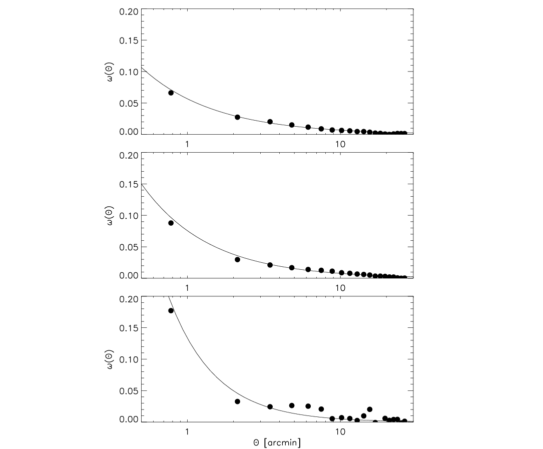
The autocorrelation functions are necessary in order to estimate the covariance matrix of the cosmic magnification. The standard power law model has been used to fit the correlation functions for the different galaxy populations. Figure 2 shows the fit for the three background populations listed in Table 1. Although the amplitude and shape agree with previous measurements in the literature (McCracken et al. (2008)) the integral constraint has not been determined here. This should only lead to a minor change in the covariance matrix since most of the contribution come from the small angular scales (less than 10 arcminutes).

5 Complementarity with cosmic shear

5.1 Signal-to-noise

The cosmic magnification and shear have different sources of sampling and statistical noise and this section is devoted to the signal-to-noise comparison of the two statistics for the same galaxy population. We compare magnification to the cosmic shear top-hat variance, defined as:

\langle\gamma^{2}\rangle={9\over 2\pi}\Omega_{m}^{2}\int s{\rm d}s\int{\rm d}w{g^{2}(w)\over a^{2}(w)}P_{3D}\left({s\over f_{K}(w)};w\right){J_{1}^{2}(\theta s)\over(s\theta)^{2}}

(46)

where $J_{1}(\theta s)$ is the first order Bessel function of the first kind. The corresponding covariance matrix has been calculated using the equation derived in Schneider et al. (2002). We consider two different background galaxy populations, at $z=[0.7,1.0]$ and $z=[1.1,1.4]$ . The number count used for the cosmic shear is the total number count for that redshift slice summed over all magnitude bins. For the magnification, the chosen magnitude range is $m=[23.5,24.5]$ and $m=[21.5,22.5]$ for the low and high redshift background respectively. The foreground population is at $z=[0.1,0.6]$ with $m=[21.5,24.5]$ . The corresponding $\alpha(m)$ and number count densities are shown in Table 1.

Figure 3 shows the signal-to-noise as function of scale for the cosmic magnification and shear. It is very interesting that using similar galaxy populations, shear and magnification are measured with similar precision. There is only a factor 2 difference, which can be further reduced from the use of combined magnitude slices for the magnification for the same source redshift, although it is not the goal of this work to investigate optimal estimators of cosmic magnification. The signal-to-noise difference between magnification and shear shown in Figure 3 is in agreement with the results from ray-tracing simulations (Takada & Hamana (2003)). Figure 4 shows that the intrinsic clustering in the cosmic magnification covariance matrix leads to significant cross-correlation between scales which dominates at large angular separation. This is why the cosmic magnification signal-to-noise decreases for scales larger than $10$ arc-minutes, where Poisson noise is negligible (see Figure 3).

5.2 Cosmological constraints

In order to test the ability of cosmic magnification to constrain the cosmological parameters, we take $b=1$ and the likelihood of cosmological models for a range of values of $\Omega_{m}$ and $\sigma_{8}$ are calculated. A fiducial model is chosen with $\Omega_{m}=0.3$ , $\Omega_{\Lambda}=0.7$ and $\sigma_{8}=0.8$ , and the covariance matrix given by Eq. 40 including the shot noise is calculated. The foreground redshift slice is chosen as $z=[0.1,0.6]$ and the background population is the same as for the two cases shown in Figure 3. The survey area is $A=1500$ square degrees. For the comparison, the shear has been calculated using the same background population as for the magnification but with no magnitude restriction (therefore shot noise is decreased compared to magnification). The results are shown in Figure 5. As it was anticipated in the previous section, the performance of the two techniques is relatively similar. Note that a 50% of the area (750 sq.deg.) used for magnification and 50% used for shear performs better than 100% of the area used for any of the shear or magnification taken alone. One should also note that degeneracy-breaking in the $\Omega_{m}$ - $\sigma_{8}$ parameter space for the combined shear-magnification arises because of the pre-factor $\Omega_{m}$ in Eq. 9, while the shear scales as $\Omega_{m}^{2}$ . In a companion paper (Hildebrandt et al. (2009a)), we presents the first measurement of cosmic magnification on galaxies. The source galaxies are Lyman-break Galaxies (LBG), selected at high redshift using the dropout technique as described in Hildebrandt et al. (2009b). This technique provides a robust way of separating background and foreground galaxies. The signal was measured for a wide range of slopes $\alpha$ which confirms the cosmological origin of the signal, similar to Scranton et al. (2005).

The main limitation for the use of cosmic magnification as a cosmology probe is the explicit dependence on the galaxy biasing, which in general cannot be assume to be $b=1$ or even constant with scale. There is however a remarkable complementarity with cosmic shear which can be exploited in order to measure the cosmological parameters. The auto-correlation function of the foreground population is indeed given by

\xi_{N}(\theta)=2b^{2}\int{\rm d}w~{p^{2}_{f}(w)\over f_{K}^{2}(w)}\int s{\rm d}s~P_{3D}\left({s\over f_{K}(w)};w\right)~J_{0}(\theta s),

(47)

and when combined with Eqs. 9 it provides an independent measurement of the usual shear two-points correlation function (Eq. 46) proportional to $\propto\sigma_{8}^{2}\Omega^{2}_{m}$ , which does not depend on galaxy biasing. The new estimator can be written as:

\xi_{\mu}(\theta)={w_{12}^{2}(\theta)\over\xi_{N}(\theta)}.

(48)

Such measurement uses photometry data only and does not rely on any shape measurement. The approach is similar to Van Waerbeke (1998) who showed that the combination of the shear with number counts provide constraints on the galaxy biasing and cosmology. In that paper it was shown that the equivalent of Eq. 9 was the cross-correlation between the shear of distant galaxies and the number counts of the foreground galaxies:

	$\displaystyle\langle M_{\rm ap}N_{\rm ap}\rangle$	$\displaystyle=$	$\displaystyle 3\pi b~\Omega_{m}\int{s{\rm d}s\over 2\pi}\int{\rm d}w{g(w)\over a(w)}{p_{1}(w)\over f_{K}(w)}\times$		(49)
			$\displaystyle P_{3D}\left({s\over f_{K}(w)};w\right)I^{2}(\theta s),$		(50)

where $I(\theta s)$ is the Fourier transform of the aperture filter. The first practical implementation combining shear and number counts was very promising (Hoekstra et al. (2002)).

The advantage of Eq. 9 over Eq. 50 lies in the fact that the cosmic magnification is completely independent of residual systematics inherent to shear measurement. It shows that the combined use of cosmic shear, magnification and number count statistics could be optimized in order to measure the cosmological parameters and simultaneously identify and reduce the systematics. Among the systematics which affect the shear and not the magnification one can mention the shear calibration and additive bias, and the intrinsic alignment which couples galaxy orientation over a large redshift range (Hirata & Seljak (2004)). High order shear statistics are particularly sensitive to intrinsic alignment which could eventually completely dominate the signal in some situations (Semboloni et al. (2008)).

Another nice feature of cosmic magnification is the possibility for exploiting faint distant galaxies for weak lensing, galaxies for which the shape cannot be measured, and therefore would not be used otherwise. This is the case for instance for LBGs which can be identified at very large redshift using the dropout technique in optical bands. Hildebrandt et al. (2009a) have successfully measured the magnification on redshift $z=3,4,5$ LBGs. This provides a very interesting observational window for future deep large surveys such as LSST and JDEM. With cosmmic shear measurement alone, a large fraction of the detected objects in those surveys would not be used for weak lensing studies. The combination of shear and magnification enables the possibility to use all detected objects (including the faint and/or high redshift galaxies and quasars) to probe dark matter from weak lensing.

Like cosmic shear, the cosmic magnification can be measured at various source redshifts, for various lens redshift, and for different magnitude bins. A study which would combine shear and magnification with a tomographic approach is left for a forthcoming study.

6 Conclusion

This paper is a preliminary study of the cosmological applications of the cosmic magnification effect. A general expression for the covariance of the magnification estimator was derived, which is the first step towards parameter measurement forecast. The CFHTLS Deep survey was used to forecast the precision of magnification measurements for future surveys and compared to the cosmic shear measurements. Although cosmic magnification has a lower signal-to-noise than cosmic shear, the former still contains useful cosmological information which should be exploited in future surveys, since to a large extend it will be obtained for free. Note that the Eddington bias (Eddington (1913)) has not been discussed in this study, but it can be easily accounted for (Hildebrandt et al. (2009a)).

In many respects, shear and magnification appear as complementary probes of the dark matter distribution. They are sensitive to completely different observational systematics, therefore they can be used as redundant measurements for a better control of the residual systematics. Magnification is also not sensitive to intrinsic alignment/shear correlations which is known to be a major source of non lensing signal for shear tomography. Some techniques have been proposed to remove intrinsic alignment using shear information only (e.g. Joachimi & Schneider (2008)), cosmic magnification could certainly help measuring it.

Although magnification is often presented as a difficult measurement, it is certainly not more difficult than galaxy shape measurement, moreover, future lensing surveys will have to have high precision photometry in order to deliver precise photometric redshifts. It is therefore natural to envision forthcoming surveys combining both measurements, however it is not clear at this stage that current plans for future surveys are yet optimal for redshift measurements. The main source of systematics for photometric redshift results from biases in the photometry. This could come from 1) incorrect calibration 2) improper color coverage or 3) small angular scale galactic and extragalactic dust extinction. Point 1) could be addressed with space-based photometry and/or partial spectroscopic followup. Point 2) could be easily addressed with an increase of wavelength coverage and/or number of filters. The importance of point 3) is unclear at the moment, although recent results from the SLOAN suggest the effect is small (Menard et al. (2009)) and chromatic signature could certainly help to disentangle weak lensing from dust extinction. At this stage, further work is necessary in order to explore in more detail the potential of cosmic magnification, in particular tomographic magnification with varying lens and source redshifts look promising. Only then, adjustments to future lensing missions could be envisioned for a better photometric redshift measurements. The explicit dependence of magnification on galaxy biasing is not a major source of concern since it can in principle be constrained from magnification tomography with varying source redshift and fixed lens redshift, moreover the combination with galaxy angular correlation functions and cosmic shear provides a direct measurement of biasing.

One should note that the detection of magnification on LBGs (Hildebrandt et al. (2009a)) is already a strong proof of concept, in that one can now measure magnification on very high redshift galaxies, in a regime where lensing is not sensitive to the exact value of $z_{s}$ . The background/foreground separation is also much easier to perform, virtually free of any contamination, and error in the foreground redshift distribution is probably not as problematic as if the redshift bins were close. This would for instance make a strong case for deep u or g coverage in order to identity redshift $3$ and $4$ dropouts with better accuracy.

The measurement of weak lensing without relying on galaxy shapes provides definitely an interesting complementary approach to cosmic shear, although it is clear it will not replace it. The main idea developed in this paper is that shear surveys could also perform magnification measurements with minor upgrades in the instrument design in order to make photometric redshift more reliable, and the scientific gain is potentially substantial. Current surveys will certainly significantly contribute in the exploration of this new direction ²² 2 CFHTLS, DES, PanSTARRS, KIDS-VISTA. It also enables wide field spectroscopic surveys such as ADEPT to perform weak lensing measurements independently from wide-field imaging surveys.

acknowledgements

I would like to warmly thank Istvan Szapudi and Jonathan Benjamin for discussions on angular auto and cross-correlation functions at the beginning of this work. It is a pleasure to thank Hendrik Hildebrandt, Martin White and Catherine Heymans for comments on the manuscript. Support from NSERC, CIfAR and CFI is also acknowledged.

References

Bartelmann (1995) Bartelmann, M., 1995, A& A, 298, 661.
Benjamin et al. (2007) Benjamin, J., Heymans, C., Semboloni, E., et al., 2007, MNRAS, 381, 702.
Bridle et al. (2008) Bridle, S., et al., 2008, astro-ph/08021214.
Coupon et al. (2009) Coupon, J., Ilbert, O., Kilbinger, M., et al., 2009, astro-ph/08113326
Eddington (1913) Eddington, A.S., 1913, MNRAS, 73, 359.
Erben et al. (2009) Erben, T., Hildebrandt, H., Lerschter, M., et al., 2009, A& A, 493, 1197.
Fu et al. (2008) Fu, L., Semboloni, E., Hoekstra, H., et al., 2008, A& A, 479, 9.
Heymans et al. (2006) Heymans, C., Van Waerbeke, L., Bacon, D., 2006, MNRAS, 368, 1323.
Hildebrandt et al. (2009a) Hildebrandt, H., Van Waerbeke, L., Erben, T., 2009a, astro-ph/0906.1580
Hildebrandt et al. (2009b) Hildebrandt, H., Pielorz, J., Erben, T., et al., 2009b, A& A, 498, 725.
Hildebrandt et al. (2008) Hildebrandt, H., Wolf, C., Benitez, N., 2008, A& A, 480, 703.
Hirata & Seljak (2004) Hirata, C., Seljak, U., 2004, PhRvD, 70, 3526.
Hoekstra et al. (2002) Hoekstra, H., Van Waerbeke, L., Gladders, M., et al., 2002, ApJ, 577, 604.
Hoekstra & Jain (2008) Hoekstra, H., Jain, B., 2008, ARNPS, 58, 99
Hu (1999) Hu, W., 1999, ApJ, 522, L21
Huterer et al. (2006) Huterer, D., Takada, M., Bernstein, G., Jain, B., 2006, ApJ, 366, 101.
Ilbert, O., et al. (2006) Ilbert, O., Arnouts, S., McCracken, H., et al., 2006, A& A, 457, 8411.
Joachimi & Schneider (2008) Joachimi, B., Schneider, P., 2008, A& A, 488, 829.
Landy & Szalay (1993) Landy, S., Szalay, A., 1993, ApJ, 412, 64.
Massey et al. (2007) Massey, R., Heymans, C., Berger, J., et al., 2007, MNRAS, 376, 13.
McCracken et al. (2008) McCracken, H., Ilbert, O., Mellier, Y., et al., 2008, A& A, 479, 321.
Menard et al. (2009) Menard, B., Kilbinger, M., Scranton, R., 2009, astro-ph/0903.1231
Moessner & Jain (1998) Moessner, R., Jain, B., 1998, MNRAS, 294, L18.
Munshi et al. (2008) Munshi, D., Valageas, P., Van Waerbeke, L., Heavens, A., 2008, Phys.Rep., 462, 67.
Narayan (1989) Narayan,R., 1989, ApJ, 339, L53.
Schneider et al. (1998) Schneider, P.; van Waerbeke, L.; Jain, B.; Kruse, G., 1998, MNRAS, 296876.
Schneider et al. (2002) P. Schneider, L. van Waerbeke, M. Kilbinger, and Y. Mellier. ApJ, 396:1, 2002.
Scranton et al. (2005) Scranton, R., Menard, B., Richards, G., et al., 2005, ApJ, 633, 589.
Semboloni et al. (2008) Semboloni, E., Heymans, C., Van Waerbeke, L., Schneider, P., 2008, MNRAS, 388, 991.
Semboloni et al. (2007) Semboloni, E., Van Waerbeke, L., Heymans, C., et al., 2007, MNRAS, 375, 6.
Takada & Hamana (2003) Takada, M., Hamana, T., MNRAS, 346, 949, 2003.
Van Waerbeke (1998) Van Waerbeke, L., 1998, A& A, 334, 1.