Mechanics of reversible unzipping
Abstract.
We study the mechanics of a reversible decohesion (unzipping) of an elastic layer subjected to quasi-static end-point loading. At the micro level the system is simulated by an elastic chain of particles interacting with a rigid foundation through breakable springs. Such system can be viewed as prototypical for the description of a wide range of phenomena from peeling of polymeric tapes, to rolling of cells, working of gecko’s fibrillar structures and denaturation of DNA. We construct a rigorous continuum limit of the discrete model which captures both stable and metastable configurations and present a detailed parametric study of the interplay between elastic and cohesive interactions. We show that the model reproduces the experimentally observed abrupt transition from an incremental evolution of the adhesion front to a sudden complete decohesion of a macroscopic segment of the adhesion layer. As the microscopic parameters vary the macroscopic response changes from quasi-ductile to quasi-brittle, with corresponding decrease in the size of the adhesion hysteresis. At the micro-scale this corresponds to a transition from a ‘localized’ to a ‘diffuse’ structure of the decohesion front (domain wall). We obtain an explicit expression for the critical debonding threshold in the limit when the internal length scales are much smaller than the size of the system. The achieved parametric control of the microscopic mechanism can be used in the design of new biological inspired adhesion devices and machines.
Key words: Unzipping, Adhesion, Peeling, Hysteresis, DNA, Gecko, Calculus of Variations, -convergence.
Introduction
Adhesion phenomena are governed by complex energy exchanges between multiple scales representing hierarchical structures. The phenomenological modeling of adhesion has been successful in describing a variety of experimentally observed static and dynamic regimes (see [9, 13, 23, 4]). The phenomenological models, however, are of a black box type and have limited predictive power outside of a particular range of parameters. More importantly, they can not be used for the microstructural optimization of the artificially created adhering materials and nanorobotics devices. It is therefore of interest to develop a multi-scale approach linking the microscopic attachment-detachment mechanisms with the macroscopic phenomenological parameters. This step is crucial for the analysis of a variety of adhesion related phenomena from fiber decohesion in composites [16, 17] and crazing/peeling phenomena in polymers [27, 13], to the activity of focal adhesions involved in cell motility [8, 18, 7] and the low temperature denaturation of single molecule DNA [22].
In this paper we contribute to this general task by considering the minimal model accounting for the interplay between elasticity and cohesion. While this model captures only the most important effects associated with quasi-static decohesion, it has the advantage of being amenable to a completely transparent mathematical analysis allowing one to study how macroscopic responses vary depending on the microscopic parameters. We focus on the case when the debonding is reversible. This type of decohesion, also known as unzipping, is crucial for the working of a variety of biological systems ([26]), in particular, for the functioning of the self-similar fibrillar Gecko’s hair([12, 21, 30]). The irreversible version of the model, which is more adequate for the description of decohesion in conventional engineering materials, will be presented in a separate paper. For a general comparison of reversible and irreversible fracture see [6].

According to typical observations the process of reversible decohesion due to quasi-static point loading includes three main stages ([13] and references therein). First the system behaves elastically until decohesion begins. Then there is a steady state incremental evolution of the decohesion front. Finally, at a critical threshold, the system undergoes a sudden transition to the fully debonded configuration. Similarly, if the system is unloaded from the fully debonded state, there exists an unloading threshold beyond which a finite portion of the adhesive layer suddenly reattaches to the adhesive background. The whole phenomenon is usually hysteretic with different attachment and detachment thresholds.
In an attempt to reproduce this basic behavior we consider a chain of massless points connected by harmonic shear springs. The particles are attached to a rigid support by breakable elastic links (see Fig.1) which mimic, depending on the parameters, either direct molecular interactions or interactions through the fibrillar adhesive layer with internal elasticity. For simplicity we neglect the bending stiffness of the elastic layer which could be accounted for by adding elastic interaction of next to nearest neighbors [16, 20]. We consider a quasi-static transversal point loading of the otherwise free layer in a hard device and study the rate independent evolution of the emerging debonding front which can be viewed as a domain wall separating bonded and debonded phases [22]. The reversal of the front direction represent the switch between zipping and unzipping.
Similar discrete models of the Frenkel-Kontorova type have been used previously in the analysis of lattice trapping of cracks in crystals [14], interfacial wetting [15] and other phenomena where an on site potential with sublinear growth competes with an elastic coupling of the elements [2]. In connection to the duplication and transcription of the DNA an approach of this type was first proposed by Peyrard and Bishop who applied it to the modeling of equilibrium melting phase transition (see the review [22]). Our model can be viewed as a purely mechanical version of the Peyrard-Bishop model where we go beyond global minima of the energy (zero temperature limit) and investigate the structure of the whole energy landscape (see also [28]). Our use of the simplified piece-wise quadratic approximation for the on site potential allows us to formulate the main results in the analytic form.
We use an incremental energy minimization approach and solve the finite dimensional variational problem for each value of applied displacement. Due to the simplicity of the cohesive potential we are able to find all equilibrium configurations and identify those representing global and local minima of the energy. Our analysis shows that the local minimizers of the energy always have a single decohesion front. The metastable configurations, forming separate branches parameterized by the loading parameter, can abruptly end. The absence of continuity leads to the necessity of ‘dynamic snapping’ from one branch to another. While these events may be dissipative, they do not prevent overall reversibility (see also [12, 21, 30]).
We discuss two evolutionary strategies. One strategy assumes an overdamped gradient flow dynamics and can be viewed as a vanishing viscosity limit (maximum delay convention, e.g. [25, 6]). The other strategy assumes that the system always remains in the global minimum of the energy (Maxwell convention). For these two models we establish the existence of the thresholds separating the regime of incremental propagation of the decohesion front from the regime of a sudden and massive decohesion representing a size effect. When we restrict the evolution of the system to the global minimization of the energy, the loading and unloading thresholds coincide. When instead we allow the system to follow the maximum delay convention and explore the set of marginally stable configurations, the two thresholds become different. The comparison with experiments shows that it is the vanishing viscosity solution which reproduces the observed adhesion hysteresis most faithfully ([13, Chapter 3]).
We then develop a continuum analog of our finite dimensional microscopic model, interpreting it as a formal -limit [1, 5]. While the limiting functional, constructed in this way, usually captures only the global minima in the original discrete problem, in our case it also agrees with a point wise limit and therefore preserves the local minima. To prove this fact we perform a systematic study of all metastable solutions of the continuum problem. While the continuum model is much more transparent mathematically and allows one to obtain the values of all relevant thresholds in explicit form, the strongly discrete limit remains important for some applications, in particular, for the modeling of the DNA [22].
The primary goal of our simplified model is to elucidate how macroscopic responses depend on the microscopic parameters. The continuum version of the model contains only one non-dimensional micro-parameter measuring the propensity of the adhesive layer to dynamic snapping. We show that the degree of localization of the decohesion front increases as decreases which is revealed macroscopically as a transition from quasi-ductile to quasi-brittle behavior. In the limit , which corresponds to the disappearing of an internal length scale, we obtain an explicit expression for the critical debonding force, which is in principle a measurable parameter [28]. In general, we expect that the achieved parametric control in the simplified microscopic setting can be used in the design of the prototypical molecular devices. We are fully aware, however, that there is long way between the toy models of the type considered in this paper and the realistic description of the particular biological systems (gecko, DNA, etc.)
The paper is organized as follows. In Section 1 we introduce our discrete model and present an analytical description of all stable and metastable configurations corresponding to a given value of applied displacement. In Section 2 we derive the -limit of the discrete model and classify the local minimizers of the limiting problem. In Section 3 we study two different responses of the discrete model to monotonous and cyclic loading, one overdamped and another nondissipative. In the dissipative case we compute the associated heat to work ratio and construct the hysteresis loops. Finally, in Section 4 we show how the main features of the cohesion/decohesion hysteresis vary as one goes from discrete to continuum description and present the results of the detailed parametric study of the model. In the Appendices we collect mathematical results of technical nature.
1. Microscopic model
Consider a discrete chain containing points which are connected by linear elastic springs with reference length . Each point is also connected to a rigid substrate by a breakable spring. In this maximally simplified setting one can deal with two prototypical problems: pull out test (e.g. [17]) and pull off or peeling test (e.g. [20]). For determinacy, we shall focus on the peeling problem and assume that the points move orthogonally to the substrate (see Fig.2).

Denote by the vertical displacements of the particles from their reference positions. The elastic energy of the connecting linear springs can be written as
| (1.1) |
where is the (shear) modulus and For the energy of the breakable springs we assume the simplest form
| (1.2) |
where is the longitudinal elastic modulus, are the normalized displacements, and is the breaking threshold. The total energy of the chain can be written as
| (1.3) |
We load the chain in a hard device, meaning that the (normalized) displacement of the first spring is prescribed
| (1.4) |
The energy can be rewritten in a more compact form. To this end we introduce a vector distinguishing ‘bonded’ and ‘de-bonded’ springs
| (1.5) |
and construct the diagonal matrix
In what follows it will be convenient to use the following notations: - the displacement vector, - the vector with , and - the first vector of the canonical basis in . We also introduce the tri-diagonal matrix
By using the above notations, we can rewrite the dimensionless total energy (1.3) in the form
| (1.6) |
where
| (1.7) |
and is the total number of debonded springs. The dimensionless energy (1.6) depends on two scaling parameters: and
| (1.8) |
The main physical nondimensional parameter of the problem, , implicitly characterizes the toughness of the breakable bonds. In particular, by decreasing we increase the cohesion energy. The geometrical parameter is a measure of discreteness and would mean for us the ‘macroscopic’ or ‘continuum’ limit (see Section 2).
To find the equilibrium state of the chain at a given , it is natural to first minimize the elastic energy at a fixed configuration of debonded springs . We obtain the following minimization problem
| (1.9) |
The necessary conditions of equilibrium can be written as
| (1.10) |
where
is the Lagrange multiplier, representing the external force acting on the first point of the chain. The stability of these equilibrium configurations is ensured by the positive definiteness of the Hessian matrix which immediately follows from (1.7). We can then conclude that all solutions of (1.10) are local minima of the energy.
The linear equations (1.10) can be solved formally which allows us to represent all metastable equilibrium configurations by the formulas
| (1.11) |
| (1.12) |
| (1.13) |
We observe that the variables given by (1.12) decrease as the index increases. This follows from the fact that the column elements in the inversions of diagonally dominant tri-diagonal matrices necessarily decrease (see e.g. [19]). Therefore in each metastable configuration it is necessarily the first springs that are debonded while the remaining are bonded. This observation allows one to write the following analytical representation for the displacement field (see Appendix A for details)
| (1.14) |
Here
| (1.15) |
is the stress,
| (1.16) |
is the effective elastic modulus, and is one of the two solutions of the equation
| (1.17) |
Since the equilibrium properties are represented by even functions of , the particular choice of the solution in (1.17) is irrelevant.
The energy of the metastable configurations can be written as
| (1.18) |
In order to be admissible, the configurations (1.14) must respect the compatibility condition requiring that all bonded springs have and all debonded springs have . This condition is equivalent to a restriction on . To obtain this restriction we compute the value of the loading parameter corresponding to and the value corresponding to . We obtain
| (1.19) |
We call the interval the stability domain of a solution with a given geometry of a crack . In general, several crack geometries may be compatible with a given load . The detailed study of the obtained solutions, in particular the specialization of the global minimizers, will be postponed till Section 3.
2. Macroscopic problem
In most applications the parameter is a large number. Therefore it is of interest to describe the continuum limit of the discrete model formulated in the previous section. As a first step we can look at the point-wise limits of the discrete solutions (1.14) as . To compute these limits we introduce
the coordinate of the th spring and define the following normalized variables:
By assuming that in the limit the parameter is finite we obtain from (1.15)
| (2.1) |
It is also easy to see that
| (2.2) |
This means that for each value of the stability domain shrinks in the continuum limit to a point. For the limiting displacement field we obtain
| (2.3) |
The value of the continuum energy of a metastable state can now be computed from the formula
| (2.4) |
Here we used the limiting relation between the stress and the length of the debonded region
| (2.5) |
To interpret these results correctly, we can independently look at the limit of the variational problem (1.9) as . To this end we can define the space of piecewise constant functions on
and rewrite the discrete energy functional (1.3) in the form
Next we can define as the subset of the functions such that there exists which satisfies
| (2.6) |
Clearly, and we rewrite the original functional in the form
| (2.7) |
where now . It is easy to see that all (local and global) minimizers of on can be described in terms of the corresponding minimizers of on which makes the two problems equivalent.
We can now study a point-wise limit of the functional (2.7). It is straightforward to see that this finite dimensional variational problem converges as to the infinite dimensional problem for the continuum functional
| (2.8) |
which is defined on the space In Appendix B we prove that the point-wise convergence automatically implies - convergence. In particular, this guarantees that the global minimizers of (2.8) can be viewed as the continuum limits of the global minimizers of (2.7).
The next question concerns the status of the local minimisers of (2.8). We say that is a local minimizer of if there exists such that for every with we have . In the important case we can prove (see Appendix C) that is a local minimizer of if and only if it coincides with a solution of the following system:
| (2.9) |
at , where is a local minimizer of the function . In the case there is only one minimum given by the solution of the Euler-Lagrange equation in with the boundary conditions and . In the special case there are two solutions, namely, the solution of the differential equation and the homogeneous solution which means that the detached set can be either empty or coincide with the whole interval .
The solution of the linear equations (2.9) can be computed explicitly. It is easy to show that they are given exactly by the formulae (2.3). This means that the limit of the metastable branches of the discrete model coincides with the metastable solutions of the continuum model. Therefore besides ensuring convergence of the global minima our pointwise limit also preserves the local minimizers.
3. Dynamic strategies
In the previous sections we found for each value of the loading parameter a variety of the accessible metastable configurations. Suppose now that the value of the loading parameter is changing quasi-statically. Then the choice of a particular local minimum occupied by the system at each value of the loading parameter is controlled by dynamics. Of a particular interest are the two evolutionary strategies. The first one represents the vanishing viscosity limit of the corresponding viscoelastic (overdamped) problem (e.g. [25]). In this case the system stays in a given metastable state till it becomes unstable (maximum delay convention). The second strategy imposes that the system is always in the global minimum of the energy (Maxwell convention). This behavior can be viewed as the zero temperature limit of the hamiltonian (underdamped) dynamics.
3.1. Viscosity solution
Suppose that the parameter is monotonically increasing starting from the value with no debonded springs (point in Fig.3). The ‘virgin’ branch becomes unstable when the first spring detaches at . According to (1.19) the decohesion starts at . The system then switches to a new metastable branch and we assume that in this new branch the only first spring, verifying , detaches whereas all other springs still remain in the elastic regime ( in Fig.3).

To check that only one spring breaks one has to study the global energy landscape and determine the steepest descending paths (see e.g. [24]). We observe that in the continuum limit, according with (2.2), a single metastable branch can be associated to each and this indeterminacy is automatically overcome. If the displacement is increased further, the debonding continues as the second spring reaches the breaking limit at ( in Fig.3). This pattern repeats itself as the subsequent springs debond one at a time. As we see the system follows a ‘pinning-depinning’ type of evolution with alternating slow elastic stages and sudden transitions between different metastable branches. This behavior, with the system switching between the branch with debonded springs to the branch with debonded springs is possible till . The numerical solution shown in Fig.3 shows that there exists a value of the external load, , such that for the only equilibrium solution is the totally debonded configuration, i.e. . Thus, when all the remaining elastic springs break simultaneously and the system jumps to the fully debonded configuration. In the case of infinite , we shall be able to find the value of the limiting threshold analytically (see Section 2).
3.2. Global minimization
To find the global minimum we have to minimize the energy of the metastable equilibrium states with respect to the parameter . Fig.4 shows by bold lines the Maxwell path for the same system as in the previous section. We observe the existence of another threshold separating the regime with a progressive debonding from the sudden jump to the fully detached configuration. Overall, the resulting stress-strain path is analogous to the one in the case of the maximum delay convention. In quantitative terms, the Maxwell loading path is lower and the transition to the fully debonded configuration is attained at a lower assigned displacement.

3.3. Dissipation
To characterize the dissipation associated with the maximum delay strategy, consider, for instance, the path b-c-d-e shown in Fig.5. We denote by the number of debonded springs at the starting equilibrium branch b-c. The subsequent branch d-e will then have debonded elements. According to the maximum delay convention, the system follows the equilibrium branch until it becomes unstable at (path b-c). Then it switches to a new branch with a smaller energy (jump c-d). To find the energy dissipated during this jump event we need to compare the energies (1.18) corresponding to the two branches and at a fixed displacement . We can write
| (3.1) |
The first term in the right hand side represents the difference of the elastic energies (area inside the triangle O-P-Q in Fig.5). The second term represents the cohesive energy accumulated by the system in the transition between the two states (it does not depend on ). The released elastic energy is partially accumulated by the system in the form of cohesion energy and the rest is dissipated. The dissipation is zero when the energy difference in (3.1) vanishes which corresponds to the Maxwell path. 11 1 Under Maxwell convention the transition to the fully debonded state also takes place without dissipation and at the decohesion energy equals the elastic energy and Instead, along the maximum delay path, represented by the points b-c-d in Fig.5, the system switches to the new branch in a dissipative way (jump c-d) and the dissipated energy is equal to the area C-c-D-d. In general, according to the maximum delay convention the area underneath the stress-strain path, representing the external work, can be decomposed into the decohesion energy represented in Fig.5 by the equal triangles of unit area (along the Maxwell path at each switching event the increment of the decohesion energy has the same magnitude as the increment of elastic energy), the accumulated elastic energy represented by the dark grey and the dissipated energy represented by the light areas between the maximum delay path and the Maxwell path.

3.4. Hysteresis
In Fig.6 and Fig.7 we illustrate the behavior of the system under cyclic loading. If the Maxwell convention is operative, there is no hysteresis and the system follows elastically the same path for loading and unloading (say, path O-A-B-A-O in Fig.6a).

If the system is unloaded, after the transition to the fully debonded state () the crack heals again at , with a sudden transformation of the cohesive energy into elastic energy. During such event a finite domain of broken springs reconnects simultaneously (path D-C-B in Fig.7a). Such snaps are indeed observed in experiments, both for loading and unloading (see [13, Chapter 3] and references therein). Experiments show, however, that the detachment and reattachment thresholds can be different with the corresponding systems exhibiting an adhesion hysteresis. This suggests that the Maxwell strategy may be less realistic than the maximum delay strategy.
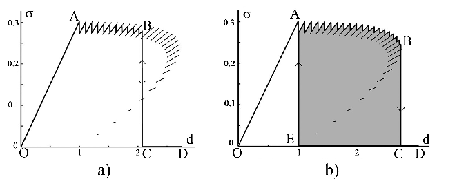
Under the maximum delay convention, if the unloading starts before the system reached the fully debonded state (), the system shows a limited hysteresis (loop O-A-B-C-D-A in Fig.6b) which disappears in the continuum limit. If we unload the chain inside this hysteresis loop (from, say, a branch ), the system first deforms elastically until when the last broken spring reconnects and the system jumps back to the branch . With further unloading the system follows this new equilibrium branch until again at another springs reconnects and so on.
In Fig.7b we illustrate the behavior of the dissipative system during the complete unloading from the fully debonded state. We remark that in contrast to the case of small cycle unloading the maximal hysteresis is preserved in the macroscopic limit.
4. Continuum behavior
We now turn to the study of the continuum solutions (2.3). Using (2.1) one can see that there exists a critical value such that for the function from (2.4) has two non-degenerate critical points where (one stable and one unstable) while for there are no such critical points.


One can also check that for the derivative , which means that the function behaves as shown in the inserts in Fig.8. Notice also that there exists another threshold such that for the global minimum is attained at the first of the two critical points, whereas for the global minimum is attained at the boundary of the domain, , describing the totally debonded configuration. Moreover, this state remains the only minimizer for the whole interval . In Fig.9 we show the stress-strain and energy-strain diagrams illustrating this behavior of the continuum solutions.
The critical value of displacement can be obtained from the equation (see Fig.8), which gives the fraction of debonded springs at . We can write explicitly
After solving this equation, we can use (2.1) to find The displacement can be obtained by first determining the fraction of debonded springs which satisfy or
Then, using (2.1), one can find
The overall comparison of Fig. 7 and Fig. 9 shows that the discrete system has a much richer set of metastable states (local minima) than its continuum analog. As increases, we observe two major tendencies: some of the branches of the local minima of the discrete system shrink to points representing the local minima of the continuum system whereas some other branches simply disappear. On the contrary, the structure of the global minimum path remains basically unaffected as .


Due to the relative simplicity of the continuum model, one can study the dependence of the response on the remaining nondimensional parameter characterizing the toughness of the adhesion layer. In Fig.10a we show three displacement fields corresponding to a given size of the crack () and to different values of the nondimensional parameter . We observe that the ‘localization’ of the crack tip predicted by our model increases as decreases. In Fig.10b we represent the force-displacement diagrams generated by the continuum model at different values of . Here the force is normalized by the debonding threshold, corresponding to
As the parameter decreases we observe an interesting evolution of the stress-strain response from an instantaneous (brittle) debonding of the whole chain to a (plasticity type) plateaux, in the case of a localized tip. In particular, one can see that the ductility of the system, represented by the overall size of the adhesion hysteresis, grows as the parameter decreases.
For the continuum system () the limit can also be interpreted as a “thermodynamic” limit because simultaneously and . In this case the normalization load vanishes,
however, the limit of the actual critical debonding force remains finite
In particular, the value of the critical force can be computed explicitly
In the context of the DNA denaturation, where our equilibrium metastable solutions represent domain walls connecting bonded and debonded states, the value corresponds to the zero temperature unzipping threshold [28].
5. Acknowledgements
The work of G.P. was supported by the Progetto Strategico, Regione Puglia: “Metodologie innovative per la modellazione e la sperimentazione sui materiali e sulle strutture, finalizzate all’avanzamento dei sistemi produttivi nel settore dell’Ingegneria Civile”. The work of L.T. was supported by the EU contract MRTN-CT-2004-505226.
6. Appendix A
To invert the tri-diagonal matrix in (1.7) we can use iterative formulas from [19]. We first relabel displacements as follows
| (6.1) |
and define the vectors and . Consider the first equations (1.10) corresponding to the debonded part of the chain. After rearrangement, these equations can be rewritten as
| (6.2) |
where we introduced the matrix and added to both sides of the first equation. The parameter is the deformation of the first bonded spring. Observe that is a Toeplitz tri-diagonal matrix which can be inverted explicitly (see e.g. [11, 19])
Since in the right hand side of (6.2) only the first and the last elements are different from zero, we are interested only in
Using the first equation of (6.2) and (1.4) we obtain
| (6.3) |
The remaining equations give
| (6.4) |
Similarly, we can reformulate the remaining equations corresponding to the bonded part of the chain in the form
where we introduced the matrix . Once again we have a tri-diagonal Toeplitz matrix and since the diagonal elements satisfy , , we can write (see again [11])
The parameter is given by the equation (1.17) and the results do not depend on the choice of one of the two solutions of this equation (indeed the equilibrium solutions are even functions of ). As in the previous case, we need only the first and the last columns of the inverse matrix
By using these formulas we obtain
| (6.5) |
7. Appendix B
Here we prove that the energy given by (2.8) is actually the -limit (with respect to the convergence in ) of given by (2.7) as .
To prove the -convergence we proceed in several steps. The first step is to find a tight lower bound. The following reasoning is standard (see [5]).
Proposition 7.1.
Assume that and for every . Then up to subsequences weakly in and . Moreover if weakly in and then
| (7.1) |
Proof.
The first assertion is trivial since implies which together with yields weak compactness of in and that any limit point of belongs to . If in addition weakly in and , then the convexity of yields
Moreover by recalling that in each and that
are the Riemann sums of the function we get
thus proving the inequality (7.1).∎
The next step is to prove the existence of a recovery sequence.
Proposition 7.2.
Assume that . Then there exists a sequence such that weakly in and
| (7.2) |
Proof.
Let and define as in (2.6). It is readily seen by convexity that . ∎
Previous statements prove that . The relationship between the minimization problems concerning the functionals and is clarified in the next theorem.
Theorem 7.3.
Let such that
| (7.3) |
then up to subsequences weakly in and
8. Appendix C
We recall that is a local minimizer of if there exists such that for every with we have .
We first show the following result.
Theorem 8.1.
If is a local minimizer of then:
- (1)
If then ;
- (2)
If then either or with .
Proof.
We begin with (2). Let , then is a non empty relatively open subset of and therefore there exists a countable collection of disjoint open intervals of , say such that
Assume by contradiction that for every , then one of the following conditions holds true
i)
ii) such that and
iii) such that and
If ii) holds then let in : since is a local minimizer we get for every such that
and by letting we have
that is in . Now, since and due to the natural boundary condition we get in the whole , which is a contradiction. Case iii) follows analogously and hence 2) is proven. In order to prove 1) suppose by contradiction that with . Then either ii) or iii) holds true and a contradiction can be obtained also in this case.∎
We can now study the relation between the local minimizers of the continuum problem (2.8) and the solution of the linear system (2.9).
Theorem 8.2.
is a local minimizer of defined by (2.8) if and only if there exists such that
| (8.1) |
and
| (8.2) |
and is a local minimizer of .
Proof.
By Theorem 8.1 we have that if is a local minimizer of then there exists such that satisfies (8.1) and (8.2). Moreover, given , there exists a given small enough , such that , the unique solution of
and
satisfies . This follows from well known results for elliptic equations with variable domains (see [3]). Hence and therefore is a local minimizer of the function .
To prove the inverse statement we have to show that if is a local minimizer for then is a local minimizer for . Let such that for every : we may choose such that if , then in and in . Hence
where if and if . Here denotes an absolute minimizer of
among all such that .
Therefore by defining
we get
An argument very close to that used in the beginning of this Appendix shows that there exists a unique such that in and in . Then, taking into account that
and
since is a local minimizer for and , we argue
thus proving the local minimality of .
∎
References
- [1] A. Braides. Gamma-convergence for beginners. Oxford University Press, 2002.
- [2] O.M. Braun and S. Kivshar The Frenkel-Kontorova Model. Springer, Berlin, 2003.
- [3] D. Bucur and G. Buttazzo. Variational methods in shape optimization problems. In: Progress in nonlinear differential equations and their applications. Birkhuser, 2005.
- [4] S. Chen, H. Gao. Bio-inspired mechanics of reversible adhesion:orientation dependent adhesion strength for non-slipping adhesive contact with transversely isotropic elastic materials. J. Mech. Phys. Sol., 55:1001–1015, 2007.
- [5] G. Dal Maso G. An Introduction to -Convergence. Birkhuser, Boston, 1993.
- [6] G. Del Piero and L. Truskinovsky. Elastic bars with cohesive energy. Cont. Mech. Thermodyn., ??:??–??, 2009.
- [7] M. Dembo, D.C. Torney, K. Saxman and D. Hammer. The reaction-limited kinetics of membrane-to-surface adhesion and detachment. Proc. R. Soc. Lond. B, 234:55–83, 1988.
- [8] V.S. Deshpande, M. Mrksich, R.M. McMeeking and A.G. Evans. A bio-mechanical model for coupling cell contractility with focal adhesion formation. J. Mech. Phys. Sol., 56:1484–1510, 2008.
- [9] M. Frémond. Contact with adhesion, chapter 4. Topics in Non smooth mechanics. Birkhuser Verlag., 1988.
- [10] A.K. Geim, S.V. Dubonos, I.V. Grigorieva, K.S. Novoselov, A.A. Zhukov, and S. Y. Shapoval. Microfabricated adhesive mimicking gecko foot-hair. Nature Materials, 2:461–461, 2003.
- [11] G.Y. Hu and R.F. Connell. Analytic inversion of symmetric tridiagonal matrices. J. Phys. A, 29:1511–1513, 1996.
- [12] A. Jagota and S.J. Bennison. Mechanics of adhesion through a fibrillar microstructure. Integrative and Comparative Biology, 42:1140–1145, 2002.
- [13] K. Kendall. Molecular adhesion and its applications. Kluver Academic, 2004.
- [14] O. Kresse and L. Truskinovsky. Lattice friction for crystalline defects: from dislocations to cracks. J. Mech. Phys. Solids., 52:2521-2543, 2003.
- [15] R. Lipowsky. Critical effects at complete wetting. Phys. Rev. B, 32:1731, 1985.
- [16] F. Maddalena and D. Percivale. Variational models for peeling problems. Interf. Free Bound., to appear, 2008.
- [17] J.J. Marigo and L. Truskinovsky. Initiation and propagation of fracture in the models of Griffith and Barenblatt. Cont. Mech. Therm., 16:391–409, 2004.
- [18] N. Mefti, B. Haussy and J.F. Ganghoffer. Mechanical modeling of the rolling phenomenon at the cell scale. Int. J. Sol. Str., 43:7378–7392, 2006.
- [19] R. Nabben. Two-sided bounds on the inverses of diagonally dominant tridiagonal matrices. Linear Algebra and its Applications, 287:289–305, 1999.
- [20] X. Oyharcabal and T. Frisch. Peeling off an elastica from a smooth attractive substrate. Phys. Rev. E, 71:0366111–6, 2005.
- [21] B.N.J. Persson. On the mechanism of adhesion in biological systems. J. Chem. Phys., 118:7614–7621, 2003.
- [22] M. Peyrard. Nonlinear dynamics and statistical physics of DNA. Nonlinearity, 17:R1-R40, 2004.
- [23] P. Podio-Guidugli. Peeling tapes, volume 13 of Mechanics of Material Forces. Ed. by P. Steinmann and G. Maugin, Springer-Verlag, 2005.
- [24] G. Puglisi and L. Truskinovsky. Rate independent hysteresis in a bi-stable chain. J. Mech. Phys. Sol., 50(2):165–187, 2002.
- [25] G. Puglisi and L. Truskinovsky. Thermodynamics of rate independent plasticity. J. Mech. Phys. Sol., 53(3):655–679, 2005.
- [26] M. Scherge and S. Gorb. Biological micro and nano tribilogy-Nature’s solutions. Springer, Berlin, 2001.
- [27] Y. Sha, C.Y. Huy, A. Ruina, and E.J. Kramer. Detailed simulation of craze fibril failure at a crack tip in a glassy polymer. Acta Mat., 45(9):3555–3563, 1997.
- [28] N. Theodorakopoulos, M.Peyrard, and R. S. MacKay. Nonlinear structures and thermodynamic instabilities in a one-dimensional lattice system. Phys. Rev. Lett., 93, 258101, 2004.
- [29] R. Thomson. Physics of fracture, volume 39 of Solid State Physics, pages 1–129. Turnbull, D., Ehrenreich, H. (Eds.), Academic Press, New York, 1987.
- [30] H. Yao, H. Gao. Mechanics of robust and releasable adhesion in biology: bottom-up designed hierarchical structures of gecko J. Mech. Phys. Sol., 54:1120–1146, 2006.