Nonlocal field correlators on the lattice in HP1 -model
B. Cheremushkinskaya 25, 117218 Moscow, Russia
Abstract
Connected two-point field strength correlators have been measured on the lattice in quaternionic projective -model of pure SU(2) Yang-Mills theory. The correlation lengths, extracted from the exponential fit for these correlators, are found to be GeV and GeV in good agreement with other existing calculations. The dependence of bilocal functions on the connector shape was studied.
The studies of nonperturbative (NP) aspects of QCD are well known to be of prime importance. This is the most interesting and rich field, albeit the most complicated one. It is commonly believed that the origin of complex NP phenomena such as confinement, chiral symmetry breaking etc is highly nontrivial structure of QCD vacuum. The important step in the NP vacuum fields investigations was undertaken in the seminal paper [1] where the gluon condensate – NP average of gluon fields over vacuum state – was introduced. This object, still playing essential role in studies of QCD vacuum structure is defined as
| (1) |
where ’s are the field strength tensors. In the QCD sum rules approach this is universal quantity (together with chiral condensate and a few higher NP averages), describing QCD vacuum. The sum rule method and idea about NP condensates have proven to be very fruitful. Using this technique masses of resonances, decay constants and other quantities of phenomenological interest were computed in good agreement with experiment. However, there are questions, which are difficult to answer in the sum rule method. In general, they arise when one is interested in such objects as potentials, excited states etc, i.e. for physical situations when one of the space-time scales characterizing the problem in question is large. It was found (in [2] on the lattice and later by other authors), that the word ”large” here has rather precise meaning: there is an important parameter, characterizing NP dynamics of vacuum fields – correlation length, which defines the spacial decay of connected gauge-invariant bilocal correlators of field tensors. It is natural to expect that original sum rule method, operating with local quantities, is not applicable to the situations where nonlocal properties of vacuum fields are essential.
The method of field correlators (MFC) [3, 4, 5] (see [6] for review) can be considered as a development of sum rules method explicitly taking into account long distance effects. The dynamical input is a set of NP field strength correlators
| (2) |
where with integration along some path, connecting the points and , are the phase factors, introduced for the sake of gauge invariance. As a matter of principle these objects can be understood as infinite power series of NP condensates and in this sense their theoretical status is absolutely equivalent to (1). But it is more convenient as is seen below, to express (2) in terms of correlation lengths. Gauge-invariant observables for QCD processes of phenomenological interest can be expressed through (2) via cluster expansion. MFC includes not only perturbative QCD at small distances, but also large distance nonperturbative effects (see [6] and references therein).
It is remarkable, that one can describe most NP QCD phenomena with high accuracy by means of the lowest two point correlator , while higher cumulants can be considered as small corrections [6]. In particular, the direct consequence of this fact is the so called Casimir scaling law for static potential between two quarks [7, 8], clearly seen on the lattice [9]. The corresponding formalism is called the Gaussian dominance approximation. Here we have single fundamental input – bilocal correlator, which has the following parametrization [3]:
| (3) |
where and are some functions of distance between two points and integration in goes along the straight lines.
At short distances the expression (3) can be expanded in powers of , the corresponding coefficients happen to be proportional the condensates of higher powers (see [10, 11, 12, 13, 14] for details). The leading nonabelian term is given by (notice that our normalization is different from that of the cited papers):
| (4) |
(thus at small distances the correlator is Gaussian as a function of ). On the other hand the NP long distance contribution can be parameterized by exponentials with the correlation lengthes and :
| (5) |
Our lattice results demonstrate that exponential behavior is a good approximation starting just from the distance of order of the correlation length (see details below), while for smaller distances the regime (4) is expected (but not explicitly seen by us due to insufficient lattice precision).
Very important source of information on field correlators are lattice measurements [2, 15]. There is an immediate problem, however. Measuring (3) on the lattice one would get piece at small distances as predicted by perturbation theory together with some NP contributions like (5) and extracting the NP part is a nontrivial task. This problem can be solved by using cooling technique (as in [2]), which allows to eliminate short range fluctuations, or by smearing procedure as in [15]. Another possibility is to expand nonlocal correlators in powers of local condensates, but needless to say that practically it is not possible to study all the series of local quantities. So, it is desirable to find some alternative approach, which allows to single out the NP signal and to compare with the other lattice methods.
For this purpose we can use an opportunity to consider modified field configurations, close in some sense to the initial configurations. A nice example of such modification is replacement of the initial SU(2) gauge theory by configurations of scalar fields representing nonlinear -model with target space being quaternionic projective space HP1. This was realized on the lattice in [16, 17], where both local objects like gluon condensate and nonlocal quantities were measured in good agreement with known results. So, the string tension calculated in terms of HP1 projected fields turned out to be very close to full SU(2) string tension, in the continuum limit. It was established, that this projection captures only NP content of gauge background, cutting contribution from perturbation theory. So, it is very natural to look at correlators of gluon fields in this approach and this is done for the first time in the present paper.
Due to lack of space we can not discuss all details of constructing HP-projected fields (see [16] for this purpose), but to be self-contained we give here the main steps. The simplest explicit parametrization of HP1 is provided by normalized quaternionic vectors
| (6) |
where H is the field of real quaternions. The states describe 7-dimensional sphere, while the HP1 space is the set of equivivalence classes of with respect to the right multiplication by unit quaternions (elements of SU(2) group)
| (7) |
Configuration , assigned to the lattice as the best possible HP1 fields approximation provides the minimum of functional
| (8) |
for given SU(2) field . The working tool for computations is link variable
| (9) |
What is actually measured is a loop made of two plaquettes (smallest rectangular contours made of four link variables) connected by the phase factors (product of links between two points) along straight lines, with different orientation of the plaquettes:
| (10) |
where is the lattice spacing.
There are two possibilities to obtain nonzero answer in (3) – when parallel planes and are perpendicular to the vector () and when planes and are parallel and lies in this plane ():
| (11) | |||
| (12) |
One attractive feature this approach is its relatively low
computational cost. Lattice simulations have been performed on PC
1.66GHz on 100 configurations (taken from [18]) at corresponding to the lattice spacing fm. The total
volume was . Other configurations with larger lattice
spacing were also used for scaling properties study.
Parametrization (5), which works very well
starting from two lattice spacing (remember that the HP1
projected fields do not contain perturbation theory contributions
at small distances) gives for correlator from (11) (see Fig.1) rather stable result GeV (or Fm) in good agreement
with [19]. The data for the correlator
(Fig.2) allow us to extract GeV (or
Fm). The preexponential factors GeV4, GeV4. We studied the
scaling properties of correlation length and found that the
dependence on the lattice spacing is almost inessential for this
quantity (see Fig.3). On the other hand, the quantity ,
which is proportional to the condensate , scales as
(see Fig.4) with MeV
and GeV4 in complete
agreement with results of [17]. The quoted
uncertainties are the standard statistical errors. For reader’s
convenience we give the values of gluonic correlation length
, obtained in other papers, in Table 1.
Table 1. Correlation length .
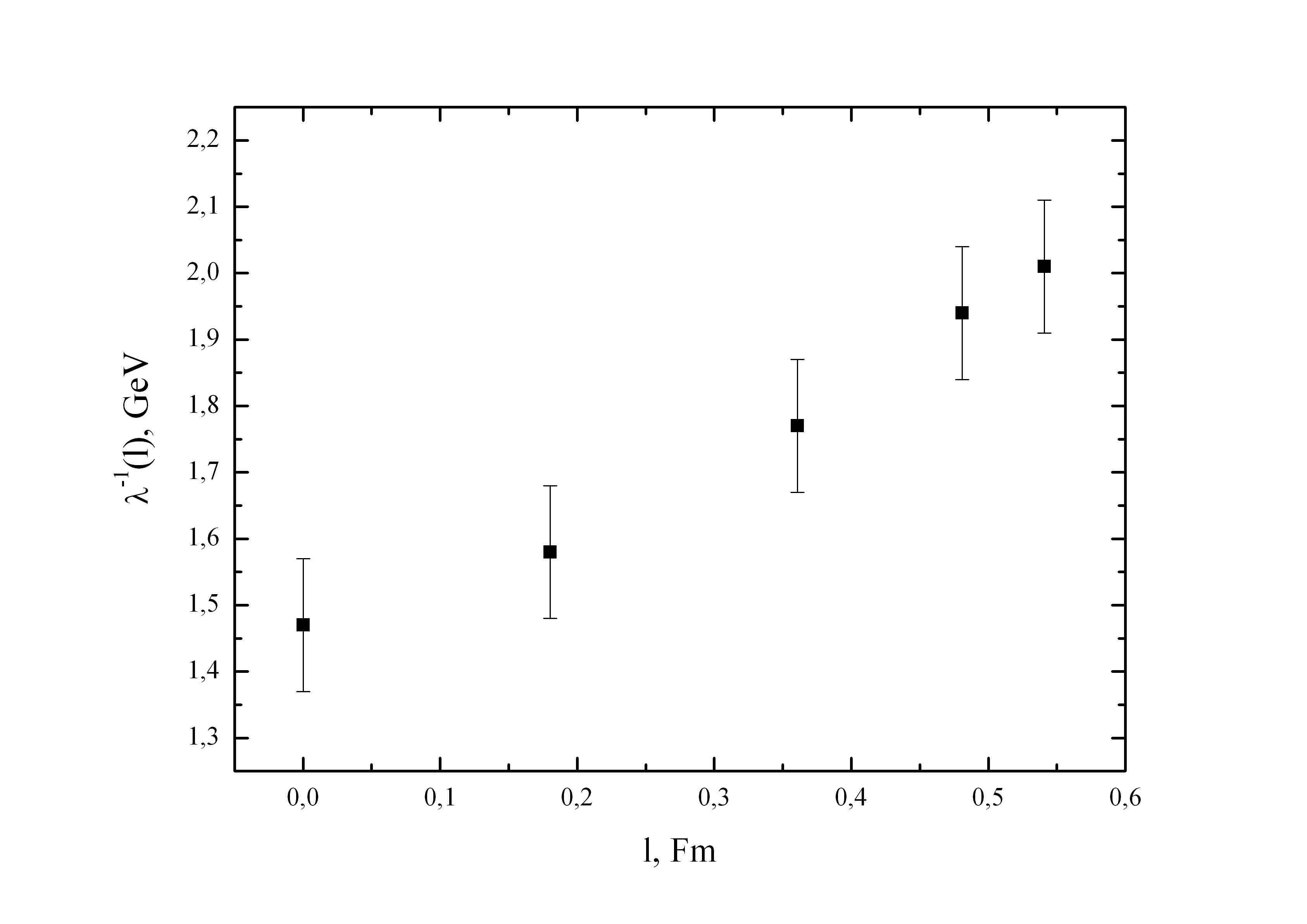
It is interesting to check how the correlators depend on the shape of curve connecting the points and . It turned out, that correlator holds the form close to exponential decay, if we replace straight connector by the U-like curve (see Fig.5). Fig.6 shows how that exponential index depends on the depth of the curve flexure. Unlike to this case of sizeable changing of correlation length for the function (by ) correlator does not preserve exponential form under the changing of the shape. We have also checked how shape of the connector influences the integral quantities. To this end, we consider the sum of two-point “U-like” and “L-like” correlators, taken over rectangle in the -plane
| (13) |
The typical contributions to the sum are shown on Fig.7. The value scales as the rectangle square for sufficiently large rectangles. The perimeter terms, also presented in , may be taken into account as - and -dependence of . The dependence of correlators on the connector shape shows as difference between and . The sum (13) as function of rectangle square is shown on Fig.8 at fixed . As turned out the difference is small:
| (14) |
so the integral quantities are almost insensitive to changing of the connector form. Another interesting question is the relation of the coefficient to the string tension (one would expect approximate equality of these quantities in Gaussian stochastic model). It will be discussed elsewhere [21].
Finally, it is natural to expect that correlators of pure electric and pure magnetic fields
| (15) |
should coincide at because of rotational symmetry of the problem. As we can see from Fig.9, it is indeed so – two lines, corresponding to logarithms of electric and magnetic correlators (15) come together at small (the error bars are within the symbols).
In conclusion, we have measured the two-points correlators of vacuum fields on the lattice in HP1 -model. This approach has allowed us to get rid of the perturbation theory contribution and to use the long-distance nonperturbative expression in the whole region of distances, beginning from two lattice spacing. Our measurements provide solid confirmation of exponential behavior for long distances of functions and , parameterizing two-point correlators. Small distance behavior is the question of separate interest, but due to insufficient precision of our lattice calculations we can not catch expected Gaussian -dependence and we do not concentrate on this problem, being interested in long-distance characteristics of two-point correlators. So, the corresponding correlation lengthes are found to be GeV and GeV in good agreement with other known calculations using completely different lattice technique. It is worth noticing that parameters turn out to be rather small, confirming the MFC picture of NP vacuum fields being weak in units of the inverse correlation length (see related discussions in [22]). We also studied the dependence of bilocal functions on the connector shape and found some decrease of the correlation length with the increasing of the connector length, corresponding to the function . In the case of the function this dependence can be established via the integral characteristic as the small difference (about 5%) between slopes of and (13) as functions of rectangle square.
The authors are grateful to F. V. Gubarev, M. I. Polikarpov and Yu. A. Simonov for helpful discussions. The research was supported by the grant for support of scientific schools NS-4961.2008.2.
References
- [1] M. A. Shifman, A. I. Vainshtein and V. I. Zakharov, Nucl. Phys. B147, 385; 448 (1979).
- [2] A. Di Giacomo, H. Panagopoulos, Phys. Lett. B285, 133 (1992).
- [3] H. G. Dosch and Yu. A. Simonov, Phys. Lett. B205, 339 (1988).
- [4] H. G. Dosch, Phys. Lett. B190, 177 (1987).
- [5] Yu. A. Simonov, Nucl. Phys. B307, 512 (1988).
- [6] A. Di Giacomo, H. G. Dosch, V. I. Shevchenko, Yu. A. Simonov, Phys. Rept. 372, 319 (2002), hep-ph/0007223.
- [7] Yu. A. Simonov, JETP Lett. 71, 127 (2000), hep-ph/0001244.
- [8] V. I. Shevchenko, Yu. A. Simonov, Phys. Rev. Lett. 85, 1811 (2000), hep-ph/0001299.
- [9] G. S. Bali, Nucl. Phys. Proc. Suppl. 83, 422 (2000), hep-lat/9908021.
- [10] S. N. Nikolaev and A. V. Radyushkin, Nucl. Phys. B213, 285 (1983).
- [11] S. V. Mikhailov, Phys. Atom. Nucl. 56, 650 (1993).
- [12] A. G. Grozin, Int. J. Mod. Phys. A10, 3497 (1995), hep-ph/9412238.
- [13] A. E. Dorokhov, S. V. Esaibegian and S. V. Mikhailov, Phys. Rev.D56, 4062 (1997), hep-ph/9702417.
- [14] V. I. Shevchenko, Yu. A. Simonov, Phys.Atom.Nucl.60, 1201 (1997), hep-th/9701026.
- [15] G. S. Bali, N. Brambilla, A. Vairo, Phys. Lett. B421, 265 (1998), hep-lat/9709079.
- [16] F. V. Gubarev, S. M. Morozov, Phys. Rev. D72, 076008 (2005), hep-lat/0509011.
- [17] P. Yu. Boyko, F. V. Gubarev, S. M. Morozov, Phys. Rev. D73, 014512 (2006), hep-lat/0511050.
- [18] F. V. Gubarev, private communication.
- [19] M. Campostrini, A. Di Giacomo, G. Mussardo, Z. Phys. C25, 173 (1984).
- [20] A. M. Badalian, A. V. Nefediev, Yu. A. Simonov, JETP Lett. 88, 558 (2009), arXiv:0807.3320 [hep-ph].
- [21] V. D. Orlovsky, V. I. Shevchenko, in preparation.
- [22] Yu. A. Simonov, V. I. Shevchenko, arXiv:0902.1405 [hep-ph].