Topological susceptibility in the SU(3) random vortex world-surface model
Abstract:
The topological charge is constructed for SU(3) center vortex world-surfaces composed of elementary squares on a hypercubic lattice. In distinction to the SU(2) case investigated previously, it is necessary to devise a proper treatment of the color structure at vortex branchings, which arise in the SU(3) case, but not for SU(2). The construction is used to evaluate the topological susceptibility in the random vortex world-surface model of infrared Yang-Mills dynamics. Results for the topological susceptibility are reported as a function of temperature, including both the confined as well as the deconfined phase.
July 14 - 19, 2008
Williamsburg, Virginia, USA
1 Introduction
The random vortex world-surface model [1, 2, 3, 4, 5, 6, 7, 8] aims to describe the gluonic dynamics of the strong interaction vacuum on the basis of center vortex degrees of freedom. These vortices are closed tubes of quantized chromomagnetic flux which spontaneously condense in the vacuum, giving rise to the nonperturbative phenomena which characterize the infrared sector of strong interaction physics, namely, confinement, the spontaneous breaking of chiral symmetry and the axial anomaly.
The random vortex world-surface model, by exploring the consequences of a simplified dynamics governing a reduced, infrared effective set of (vortex) degrees of freedom, complements studies of center vortices extracted from lattice gauge configurations [9, 10, 11, 12, 13, 14, 15]. Such studies employ appropriate gauge fixing and projection procedures [9, 10, 12] to determine the vortex content of gauge configurations; having isolated the vortices, one can investigate to what extent, e.g., confinement is caused specifically by those vortices. Conversely, one can ask whether any of the characteristic strong interaction phenomena persist if vortices are removed from the lattice configurations. These investigations have yielded strong support for the vortex picture of the strong interaction vacuum; pars pro toto, results include vortex dominance of the string tension [9, 10, 12], the absence of topological charge and a chiral condensate when vortices are removed [11, 12], and a picture of the deconfining phase transition in terms of vortex percolation properties [13]. Further details, including an outlook on the relation of the vortex picture to other models of the strong interaction vacuum, can be found in the reviews [16, 17].
On the other hand, the simplified infrared effective description provided by the random vortex world-surface model permits the exploration of a wider variety of settings. For the simplest case of color, studied initially, the model was shown to exhibit both a low-temperature confining phase as well as a high-temperature deconfined phase [1], separated by a second-order phase transition [4]. The predictions of the model for the spatial string tension in the deconfined phase [1], the topological susceptibility [2] and the (quenched) chiral condensate [3] quantitatively match corresponding lattice Yang-Mills results. Building on this initial progress, the random vortex world-surface model was extended to the case of color. Studies of the confinement properties yielded a weakly first-order deconfinement phase transition [4], also seen in the vortex free energy [6], which represents an alternative order parameter for confinement. Furthermore, a Y law for the baryonic static potential was observed [5]. Spurred by recent investigations of Yang-Mills theories with a wider variety of gauge groups, aiming at a better understanding of possible confinement mechanisms [18], the confinement properties of the random vortex world-surface model were subsequently also studied for color [7] and color [8]. These studies showed that the vortex picture can accomodate such diverse color symmetries, while indicating the limitations of the very simple effective dynamics which had proven adequate in the and cases.
After these detours into investigations of other gauge groups, the present work returns to the case, widening the scope from the confinement properties studied previously, cf. above, to the topological properties. Specifically, the topological charge is constructed for model vortex world-surfaces, where some additional complications arise compared to the case. On this basis, the topological susceptibility, which determines the anomalously high mass of the meson, is evaluated as a function of temperature.
2 SU(3) center vortex color structure
Center vortices are closed tubes of quantized chromomagnetic flux in three space dimensions; correspondingly, they are described by (thickened) closed two-dimensional world-surfaces in four space-time dimensions. The quantization of flux is determined by the center of the gauge group. If one evaluates a Wilson loop corresponding to a path encircling an vortex, one obtains one of the two nontrivial center elements of ,
| (1) |
The two center elements in (1) are complex conjugates; thus, there is only one type of vortex flux, the two possible orientations of which generate the two signs in (1). This color structure nevertheless admits vortex branching, in contradistinction to the case; a vortex associated with a center phase can branch into two vortices which are each associated with the phase . This respects the Bianchi constraint (continuity of flux modulo Abelian magnetic monopoles). The presence of branchings introduces an additional complication for the evaluation of the topological charge of model vortex world-surfaces, an issue which deserves further elaboration: Evaluating the topological charge via
| (2) |
implies that a more specific description of the vortex gauge field must be given than just the Wilson loops (1). As a first step, it is useful to cast vortices in an Abelian gauge, i.e., the gauge field and the field strength are diagonal in color space. This, however, does not yet completely specify the color structure. One can further fix the gauge by allowing the vortex gauge field to be proportional only to color matrices from a certain set. Consider the following (minimal) choice,
| (3) |
so that there is one, and only one, generator for each of the possible vortex fluxes,
| (4) |
Consider now what happens at a branching of a vortex associated with into two vortices each associated with , cf. Fig. 1 (left).

diag diag
diag diag diag diag
Flux at the branching is only continuous modulo in each color component, since
| (5) |
Therefore, there is necessarily a source or sink of Abelian magnetic flux, i.e., an Abelian magnetic monopole associated with the branching. As will become more clear further below, this introduces an ambiguity into the evaluation of the topological charge which can only be remedied by deforming the monopole world-line away from the branching. The minimal choice of color matrices considered above is clearly not flexible enough to allow for such a deformation. Consider, therefore, a non-minimal choice [19] such as
| (6) |
In such a gauge, one has the freedom to disassociate monopoles from branchings, cf. Fig. 1 (right); there,
| (7) |
without the presence of any monopoles at the branching. This property makes the non-minimal description (6) suited for an unambiguous evaluation of the vortex topological charge, as opposed to the minimal description (3). Vortex world-surfaces in the following are thus described as consisting of patches which are each associated with a specific color direction from the set (6).
3 Center vortex topological charge
Vortex topological charge is generated by two geometrical features, namely, vortex world-surface intersection points and vortex world-surface writhe11 1 This is easily understood by noting that, in three dimensions, a static magnetic flux in the 3-direction is associated with the 3-component of the magnetic field, , and therefore with the field strength component . Expanding to space-time, this means that a vortex world-surface running in the 3-4 directions is associated with and, conversely, a world-surface running in the 1-2 directions is associated with . If the two intersect, there is a point in space-time which simultaneously supports nonvanishing and , and at which topological charge density is therefore generated according to (2). Similarly, if a single vortex world-surface writhes in a way which explores all four space-time dimensions, topological charge density is generated. [2, 19, 20, 21, 22]. As described further in section 4, vortex world-surfaces will, for practical purposes, be modeled as consisting of elementary squares on a hypercubic lattice. While for continuum surfaces, topological charge due to writhe is distributed continuously on the surfaces [21], on the aforementioned hypercubic model surfaces, topological charge due to writhe is concentrated onto lattice sites (as is, of course, topological charge due to vortex intersection points). Thus, at first sight, it would seem that the topological charge of vortex surfaces composed of elementary squares can be evaluated simply by considering all lattice sites in turn, at each site finding all pairs of mutually orthogonal vortex squares attached to the site, and weighting their contribution to the topological charge appropriately with , where and are the color directions, cf. (6), associated with the two squares making up the pair in question. However, the hypercubic description introduces two types of ambiguities which must be resolved before the topological charge can be evaluated in this manner.

First, whereas continuum surfaces generically intersect at points in four dimensions, random hypercubic lattice surfaces share whole line segments with a finite probability, e.g., as displayed in Fig. 2. Such features are artefacts due to the discrete set of directions available to the surfaces on a lattice. They complicate the identification of intersection points. When whole links are shared between surfaces, in general there is no unambiguous assignment of the attached elementary squares to two distinct surfaces; as a consequence, the question of whether the surfaces are actually intersecting or merely touching becomes at best nonlocal, and in general ambiguous. To resolve such ambiguities, the hypercubic surfaces are transferred to a finer lattice, and small deformations are carried out until there are no lattice links left to which four or more vortex squares are attached (links with three attached squares of course constitute bona fide branchings). The deformations are such that the deformed surfaces never deviate from the original ones by more than one-half of the original lattice spacing; therefore, on the scale of the cutoff of the infrared effective vortex dynamics, the original and the deformed surfaces are indistinguishable. In particular, all Wilson loops defined on the original configurations remain unchanged. Nevertheless, this procedure may introduce additional spurious topological charge lumps on the scale of the finer lattice, and the topological susceptibility may therefore be overestimated as a result. The corresponding systematic downward uncertainty associated with the measured topological susceptibility, cf. Fig. 3 below, is quantified by scaling with the appropriate power of the vortex density, which is expected to roughly track the topological density, and which increases appreciably in the course of the deformation procedure. This issue constitutes the chief source of uncertainty in the results of this work.
The second ambiguity present in hypercubic surface configurations was already alluded to in section 2. If Abelian magnetic monopoles are rigidly tied to branchings, their world-lines necessarily run through lattice sites. On the other hand, topological charge density is concentrated onto the sites in the hypercubic description. This coincidence of the two also creates an ambiguity; at monopoles, the color direction of the vortex surface changes, and consequently, by having a monopole precisely intersect a site carrying topological charge density, the latter can be arbitrarily modified at that site. Such precise coincidence is again an artefact of the hypercubic description, and this ambiguity is resolved by deforming all monopole lines such that they never intersect sites carrying topological charge. This is possible using the vortex color structure defined by (6).
4 Random vortex world-surface model
The assumptions underlying the random vortex world-surface model have been discussed in detail elsewhere [1, 4]; here, a short synopsis shall suffice. Vortex world-surfaces are modeled by composing them of elementary squares on a hypercubic lattice. An ensemble of such surfaces is generated using Monte Carlo methods, respecting the (Bianchi) constraint that vortex surfaces be closed at each update. The spacing of the lattice is a fixed physical quantity, representing the ultraviolet cutoff of this infrared effective model. Physically, it mimics vortex thickness; e.g., two parallel thick vortices must remain at a minimal distance in order to still be resolved as distinct. If one sets the scale by using the string tension value , the lattice spacing is . Finally, the vortex ensemble is governed by a world-surface curvature action, symbolically,
![[Uncaptioned image]](0906.1294v1/cactdef.png)
| (8) |
i.e., each instance of two vortex squares sharing a link, but not lying in the same plane costs an action increment . The lone dimensionless parameter of the model is fixed to by reproducing the relation between the deconfinement temperature and the zero-temperature string tension known from lattice Yang-Mills theory [23], .
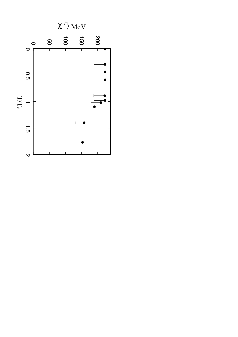
Generating a random vortex world-surface ensemble in this manner, and determining the topological charge of each configuration as indicated in section 3 leads to the result for the topological susceptibility (where denotes the four-volume) depicted in Fig. 3; the temperature is varied as usual by changing the extent of the Euclidean time dimension of the lattice, and the downward uncertainty of the measurement was estimated according to the discussion in section 3.
5 Conclusions
The raw data for the topological susceptibility collected in the random vortex world-surface model, cf. Fig. 3, are somewhat higher than measurements in lattice Yang-Mills theory [24] (cf. in particular Table 1 therein), which roughly indicate a value of around 190 MeV for the fourth root of the susceptibility at zero temperature, with values as high as 213 MeV and as low as 168 MeV reported; for finite temperatures, cf., e.g., [25]. However, there is a substantial systematic downward uncertainty inherent in the measurement of the vortex model topological susceptibility carried out in the present work. This uncertainty is a consequence of ambiguities introduced into the world-surface configurations by the hypercubic description, cf. section 3, and of the procedure employed to resolve these ambiguities. Taking this uncertainty into account leaves room for the possibility that the topological susceptibility of the random vortex world-surface ensemble is consistent with Yang-Mills theory. It should be stressed that the aforementioned ambiguities are not intrinsic to the vortex picture, but result from the specific hypercubic realization of the vortex world-surfaces adopted here for practical purposes. An alternative model description which removes the associated uncertainty could, e.g., be achieved by constructing the world-surfaces as random triangulations. In this way, by letting surfaces extend into arbitrary directions in four-dimensional space-time, the ambiguities in question are avoided. On the other hand, such a description is technically considerably more involved, e.g., in terms of generating a grand canonical ensemble of surfaces, or also in terms of the book-keeping of vortex locations.
References
- [1] M. Engelhardt and H. Reinhardt, Nucl. Phys. B585 (2000) 591.
- [2] M. Engelhardt, Nucl. Phys. B585 (2000) 614.
- [3] M. Engelhardt, Nucl. Phys. B638 (2002) 81.
- [4] M. Engelhardt, M. Quandt and H. Reinhardt, Nucl. Phys. B685 (2004) 227.
- [5] M. Engelhardt, Phys. Rev. D 70 (2004) 074004.
- [6] M. Quandt, H. Reinhardt and M. Engelhardt, Phys. Rev. D 71 (2005) 054026.
- [7] M. Engelhardt, Phys. Rev. D 73 (2006) 034015.
- [8] M. Engelhardt and B. Sperisen, Phys. Rev. D 74 (2006) 125011.
- [9] L. Del Debbio, M. Faber, J. Greensite and Š. Olejník, Phys. Rev. D 55 (1997) 2298.
- [10] L. Del Debbio, M. Faber, J. Giedt, J. Greensite and Š. Olejník, Phys. Rev. D 58 (1998) 094501.
- [11] P. de Forcrand and M. D’Elia, Phys. Rev. Lett. 82 (1999) 4582.
- [12] C. Alexandrou, M. D’Elia and P. de Forcrand, Nucl. Phys. Proc. Suppl. 83 (2000) 437.
- [13] M. Engelhardt, K. Langfeld, H. Reinhardt and O. Tennert, Phys. Rev. D 61 (2000) 054504.
- [14] R. Bertle, M. Engelhardt and M. Faber, Phys. Rev. D 64 (2001) 074504.
- [15] R. Höllwieser, M. Faber, J. Greensite, U. M. Heller and Š. Olejník, arXiv:0805.1846 [hep-lat].
- [16] J. Greensite, Prog. Part. Nucl. Phys. 51 (2003) 1.
- [17] M. Engelhardt, Nucl. Phys. Proc. Suppl. 140 (2005) 92.
- [18] K. Holland, M. Pepe, and U.-J. Wiese, Nucl. Phys. B694 (2004) 35.
- [19] J. M. Cornwall, Phys. Rev. D 58 (1998) 105028.
- [20] M. Engelhardt and H. Reinhardt, Nucl. Phys. B567 (2000) 249.
- [21] F. Bruckmann and M. Engelhardt, Phys. Rev. D 68 (2003) 105011.
- [22] G. Jordan, R. Höllwieser, M. Faber and U. M. Heller, Phys. Rev. D 77 (2008) 014515.
- [23] G. Boyd, J. Engels, F. Karsch, E. Laermann, C. Legeland, M. Lütgemeier and B. Petersson, Nucl. Phys. B469 (1996) 419.
- [24] E. Vicari and H. Panagopoulos, arXiv:0803.1593 [hep-th].
- [25] B. Allés, M. D’Elia and A. Di Giacomo, Nucl. Phys. B494 (1997) 281; erratum ibid. B679 (2004) 397.